The ground state energy of the Edwards-Anderson spin glass model with a parallel tempering Monte Carlo algorithm
Abstract
We study the efficiency of parallel tempering Monte Carlo technique for calculating true ground states of the Edwards-Anderson spin glass model. Bimodal and Gaussian bond distributions were considered in two and three-dimensional lattices. By a systematic analysis we find a simple formula to estimate the values of the parameters needed in the algorithm to find the GS with a fixed average probability. We also study the performance of the algorithm for single samples, quantifying the difference between samples where the GS is hard, or easy, to find. The GS energies we obtain are in good agreement with the values found in the literature. Our results show that the performance of the parallel tempering technique is comparable to more powerful heuristics developed to find the ground state of Ising spin glass systems.
Keywords:
Spin-glass and other random models , Numerical simulation studies, , , ,
1 Introduction
The study of spin glasses is an active and controversial area of statistical physics. In particular, the properties of these systems at zero temperature have been intensively studied in the last years. The problem of finding ground states (GSs) is a very difficult subject because of the quenched disorder and frustration that are present in most realistic spin glass models. In fact, it has even been shown that finding the GS of a spin glass in a three-dimensional lattice is an NP-complete problem [1], which means that this challenge is at least as difficult as the hardest problems of practical interest. As a consequence, many different algorithms [2, 3, 4, 5, 6, 7, 8] have been proposed to solve it, and to assess the efficiency of these algorithms is thus very important. Genetic algorithms [2] are considered as the most powerful heuristics to reach the GS of spin glass systems [9, 10]. After introduction of the triadic crossover by Pál [3, 4], different improvements have been made to combine genetic algorithms with, for example, cluster-exact approximation [5, 6] and renormalization [7]. Nevertheless, algorithms based in Monte Carlo (MC) methods, such as simulated annealing (SA) [11], multicanonical ensemble [12] and parallel tempering (PT) [13, 14], have also been used to find GSs of spin glasses. Just as genetic algorithms, they are simple to be implemented. However, MC methods are usually considered less efficient than genetic algorithms, because it is often assumed that the presence of a temperature parameter in the algorithm entails a breaking of the ergodicity that can lead to difficulties in the searching of GSs of disordered systems.
Recently, PT has been used to find the GS (see, for instance Refs. [15, 16, 17, 18, 19]), and it has been shown [15] to be more efficient than other MC based algorithms. However, the issue of the efficiency of the PT algorithm has been very briefly discussed in the literature. In this work, we tackle this point in a more systematic way by analyzing how this efficiency depends on the different input parameters of the PT. The system to which the algorithm is applied is the Edwards-Anderson (EA) spin glass model [20] in two-dimensional (2D) and three-dimensional (3D) lattices, with both bimodal and Gaussian distributions of bonds. The results show that the performance of the PT technique is comparable to more powerful heuristics developed to find the GS of disordered and frustrated systems. Furthermore, we show that the efficiency depends of certain combinations of the parameters. In particular, we find a heuristic formula that gives the minimum time (in unit of time of PT algorithm, see below) that is necessary to find the GS with a fixed probability and for a given lattice size.
The paper is structured as follows. In Sec. 2 we present the EA model and three different implementations of the PT algorithm. In Sec. 3, we determine the values of the algorithm parameters that are needed to find the GS, with a fixed average probability, for 2D and 3D EA models with bimodal and Gaussian bond distributions, for small lattice sizes. Using this, we obtain the GS energy for larger sizes and the thermodynamic limit of this quantity. In Sec. 4, we study the efficiency of the PT algorithm to find the GS of single samples. Conclusions are drawn in Sec. 5.
2 Model and Algorithm
We consider the Edwards-Anderson spin glass model [20], which consists of a set of Ising spins placed in a square or cubic lattice of linear dimension , with periodic boundary conditions in all directions. Its Hamiltonian is
| (1) |
where indicates a sum over nearest neighbors. The coupling constants or bonds, ’s, are independent random variables drawn from a given distribution with mean zero and variance one. In this paper we concentrate on the EA model with two distributions: the bimodal (EAB), and the Gaussian (EAG). In the EAB model, the bonds take only two values , with equal probability. For relatively large system sizes, and due to the fact that the bonds are independent variables, only configurations with half of the bonds of each sign are statistically significant. To preserve this feature for small sizes, we explicitly enforce the constraint
| (2) |
For systems with an odd number of bonds, we enforce the constraint for the half of the samples and for the other half. In the EAG model, the bonds are drawn from a Gaussian distribution. One important difference between these two models is that whereas for the EAG the GS of the system is unique (up to a global symmetry), the EAB has a highly degenerate GS.
In order to implement a PT algorithm [14] one needs to make replicas of the system (ensemble) to be analyzed, each of which is characterized by a temperature parameter (). The basic idea of this algorithm is to simulate independently a Hamiltonian dynamics (standard MC) for each replica, and to swap periodically the configurations of two randomly chosen temperatures. The purpose of this swap is to try to avoid that replicas at low temperatures get stuck in local minima. Thus the highest temperature, , is set in the high-temperature phase where relaxation time is expected to be very short and there exists only one minimum in the free energy space. The lowest temperature, , is set in the low-temperature phase. Within this interval we choose equally spaced temperatures, i.e. .
As mentioned above, PT is based on two procedures that are performed alternately. In the first one, a standard MC method is used to independently simulate the dynamics of each replica: in each elementary step, the update of a randomly selected spin of the ensemble is attempted with a probability given by the Metropolis rule [21]. In the second procedure, a trial exchange of two configurations and (corresponding to the -th and -th replicas) is attempted, and accepted with probability [14]
| (3) |
where and (we have taken the Boltzmann’s constant equal to one without loss of generality). As in Ref. [14], we restrict the replica exchange to the case . The unit of time in this process or PT step (PTS) consists of a fixed number of elementary steps of standard MC, followed by other fixed number of trials of replica exchange. The initial configuration of each replica is usually random but, as discussed below, other choices can endow the algorithm with some interesting features. The running time of our code, (in seconds), can be approximated by
| (4) |
where is the number of PTSs, is the number of independent runs and is a constant.
Depending on the way we combine the number of elementary steps of standard MC and the number of replica exchanges, we define three different variants of the PT algorithm. The one that we call A algorithm consists of two stages. The first is simply a SA routine implemented as follows. Starting from a random initial condition, MC steps (MCSs) of standard MC are applied to replica 1 (each MCS consists of elementary steps of standard MC). Next, the same is done successively for each replica, but taking the last configuration of replica as the initial condition of replica . The final configurations obtained are used to initialize a PT algorithm. In the second stage, we define that a PTS consists of cycles, each cycle being one elementary step of standard MC plus one replica exchange. After PTSs, the algorithm stops and its output is the configuration with the smallest energy among all configurations visited by all replicas in the simulation process.
In the second variant, that we call B, the replicas are initialized with a random configuration and the PTS consists of elementary steps of standard MC and only one replica exchange. This definition is usually chosen to reach equilibrium. After PTSs the algorithm stops and the configuration with lowest energy is stored.
Finally, a third variant, called C, consists only of the second stage of variant A, but with the initial configurations randomly chosen. After PTSs (where the PTS is defined as in A algorithm), the configuration with minimum energy is stored.
To compare the performance of the three variants proposed, we run each one of them on the same samples of the 2D EAB model (only one run for sample). We choose the values of parameters , and in such a way as to ensure that the running time of the three variants is the same. In our case, we have used , and (this choice depends on the particular implementation of each algorithm). In order to check whether the final configuration found by each algorithm is really a GS, we compare with the output of an exact branch-and-cut algorithm run on the same samples [22, 23]. The quantity we choose to compare the efficiency of the variants A, B and C, is the mean probability of finding the GS, , which we estimate as
| (5) |
where
| (6) |
is an estimation of the probability of reaching the GS for the -th sample, . In the last equation, is the number of times that GS is found for the -th sample in independent runs. Note that in this example we use . Therefore for each sample or 1. As it is shown in the appendix A, the error associated to becomes small if many samples are considered and only one run is carried out in each one of them (it is not necessary to consider many runs for sample, i.e. ).


The result of this comparison is shown in Fig. 1 for different values of and (see appendix A for a detailed calculation of the error bars). It can be seen that the performance of the three variants is very similar for all values of . However, a exhaustive analysis shows that for , the performance of B and C algorithms is a little better than the one corresponding to A and this behavior is reinforced upon increasing the lattice size [see Fig. 1 (a)]. On the other hand, by comparing the curves for in Figs. 1 (a) and (b), we observe that if is increased, the probability for A and B is the same, while for C it is a little larger. These examples show that the PT algorithm has a complex dependence with . The above comparison has been performed also for the other studied cases (2D EAG, 3D EAB and 3D EAG models) and the results are very similar to those shown in Fig. 1. The most important feature is that in the large regime, the performance of A is always worse than the other two, which means that its performance could be used as a lower bound for the B and C cases. For this reason, in the following we only analyze the performance of A. In addition, we show below that variant A presents very interesting scaling properties. To avoid confusions, we keep in the rest of this paper.
3 Results
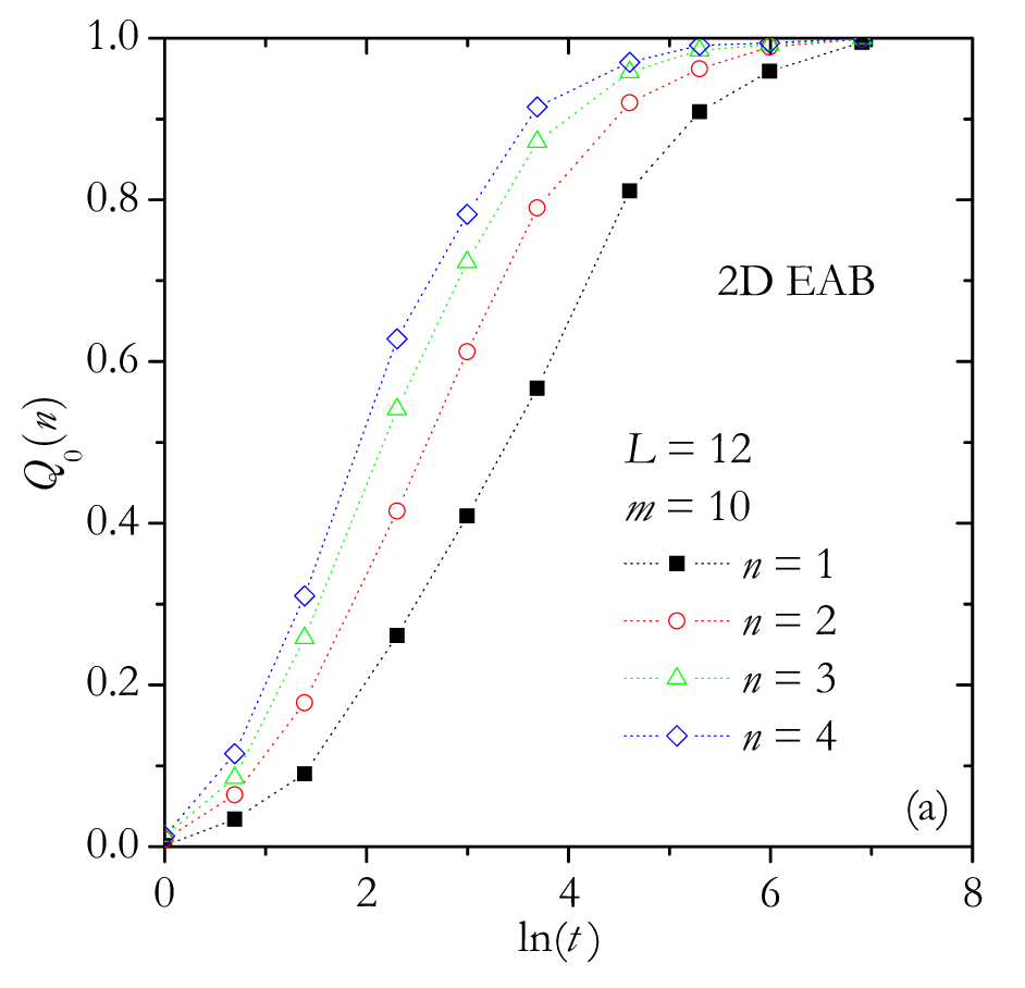
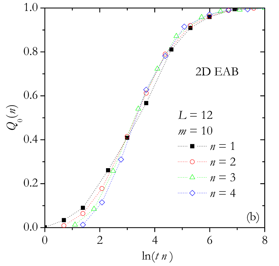
In this section we study the A algorithm for the EAB and EAG models in 2D and 3D. The first issue we address is whether it is better to use a large and one run for each sample, or several runs but with a smaller . The quantity to be studied for this purpose is , which is the sample average of the probability that a GS is found in at least one of the independent runs in the -th sample, . Figure 2 (a) shows the estimate of this quantity, , as a function of for , , and . We use samples of and . As expected, the performance improves with increasing . However, when time is rescaled to in order to compare the performances at the same running time [see Eq. (4)], independently of the number of runs, the curves approximately collapse [see Fig. 2 (b)]. The example shows that increasing the number of PTSs, has approximately the same effect as performing independent runs. This is due to the fact that, if an appropriate set of parameters are chosen, the fractions of phase space explored by the PT algorithm are similar in both cases. As this is a recurrent feature in all tested problems, in the rest of this article we take .
In the following, we first determine the range of temperatures which is globally optimal. Although for each particular problem (EAB or EAG in either 2D or 3D) is possible to determine a different optimal set, for simplicity we choose to fix the range of temperatures. Then, we focus on the number of replicas and the time . Finally, the analysis for small size allows us to predict the optimal values of these parameters for larger lattice sizes.
3.1 2D EA models
We begin by discussing the criteria for selecting a suitable range of temperature for each studied system. As mentioned above, it is important that the highest temperature is set in the high-temperature phase: , where is the critical temperature. Although for the 2D EA models , below the dynamics becomes slow [24] and the system has very long relaxation times. Then, it is reasonable to expect that the optimal should be . On the other hand, as the algorithm is designed to reach the GS, the lowest temperature should be very low (but not zero because the Metropolis rule is not efficient in that case).

As in the previous section, we run the algorithm with several different temperature ranges, on different samples per size (in the following, this number of samples is used for all 2D calculations). for the EAB model is shown in Fig. 3. We find that, if we fix the lowest temperature at , for the case the highest temperature should not be lower than . On the other hand, if we choose the highest temperature at , the lowest temperature should not be higher than . In addition, as seen for , both ranges to and to , give similar results. The conclusion is that the performance of the algorithm depends only weakly on the range of temperatures chosen under the condition that, a) the largest temperature is outside the region of slow dynamics (), and b) the lowest temperature is not too high (say, ). This conclusion is also valid for the EAG model. As the bounds mentioned are only approximate, to be sure to meet that condition, in the remaining of this subsection we use and for all the simulations.
We now discuss the dependence of probability on parameters , and . Figure 4 (a) shows the curves of probability for different lattice sizes and number of replicas. As was to be expected, for fixed values of , increases with . Thus, given that the running time is proportional to [see Eq. (4)], is reasonable to draw the curves as functions of
| (7) |
as in Fig. 4 (b). As before, when we carry out independent runs, the curves for different and fixed collapse to the same curve. This behavior shows that is a function of for fixed size [25].
The collapse observed previously can be used to find a formula, that allows us to estimate the number of PTSs that are necessary to reach the GS with a average probability . The simplest function that we have found to provide a good fit for the data has five parameters. In the following paragraphs we show, using heuristic arguments, how such a formula is obtained.


We now turn to the dependence of the curves shown in Fig. 4 (b), with the hope that they too can be collapsed onto a single curve. First, note that the inflection point is located approximately at . Figure 5 (a) shows that , the value of at , can be approximated by a linear function of (a poor fit is obtained if a linear function of is used). By fitting these points with the function
| (8) |
we obtain and ( is fixed to , but it is left as a variable in the equation because its value is different in 3D). We rescale the abscissa axis of Fig. 4 (b), using the variable
| (9) |
The denominator has been introduced to compensate for the fact that the slope at changes slightly with . Figure 5 (b) shows that, for , this rescaling indeed collapses all the curves of figure 4 (a) onto a single curve.
Furthermore, we find that all data points of Fig. 5 (b) can be fitted by the function
| (10) |
where [see figure 5 (b)]. By combining Eqs. (9) and (10), we can obtain a simple expression to predict the number of PTSs necessary to reach the GS with a given value of ,
| (11) |
Even though the rescaling proposed is not rigorous and the function Eq. (10) is chosen arbitrarily, the expression Eq. (11) will allow us to estimate the value of for each lattice size and for a given average probability with great accuracy (see Subsec. 3.3). Notice that an exponential dependence on size has also already been reported in Ref. [17], for the time that a PT algorithm needs to find the GS of a 1D spin glass model with power law interactions, in the case where the power law parameter is , which can be considered effectively as a short range interaction.
We stress that the purpose of Eq. (11) is not to provide an accurate model of the PT algorithm, but only to give a simple estimate of the number of PTSs needed to achieve a certain average probability of finding a GS. In fact, the actual obtained using this estimate can vary strongly from sample to sample (see Sec. 4).


Now, we repeat the previous analysis for the EAG model. Figures 6 (a) and (b) show the probability for different lattice sizes and number of replicas as functions of and , respectively. Even though the collapse in this case is not as good as for the EAB model, it is still very good in the region of high (. Figure 7 (a) shows as function of . As before, we fit these points with Eq. (8) and we obtain and (). A second collapsing of the data is shown in Fig. 7 (b), again for . This collapse is well fitted by the function in Eq. (10) with [see figure 7 (b)].
One difference with the EAB case is that the value of the parameter is larger, which implies that, for example, for , and , the required number of PTSs for the EAG model is two orders of magnitude larger than for the EAB model. This is also a common feature of other heuristics as genetic algorithm, where GSs are harder to obtain for Gaussian than for bimodal bond distributions. The reason is that the GS of the EAG model is unique, while it is degenerate for the EAB model, making it easier to find because any one of them is sufficient [26]. In fact, the ground-state entropy per spin for the EAB model with is approximately [27], what implies that the number of GSs is .
3.2 3D EA models
In the previous analysis for 2D lattices we have checked the GS energies obtained by PT, comparing them with the exact ones calculated with branch-and-cut algorithm [22]. But finding the GS of a 3D system is a much more difficult task, and exact algorithms available to us can only be used for small lattices (up to ). Therefore, a different strategy must be used to ensure that the configurations found by our algorithm really correspond to true GSs. The method we have used is as follows. First, we run the algorithm for a certain time , for each sample of a given set. Then, the algorithm is run anew but now duplicating the time . This is repeated many times, and thus a series of configurations, with their energies, are stored. We stop this process when, for each sample, in two successive runs the same minimum energy is obtained. Note that the process continues in all samples, while at least the minimum energy for one sample changes in two successive runs. Comparing the series of energies, we can separate them into ”easy” and ”hard” samples (the GS energy of an easy sample is obtained in a few steps of the previous process, while for a hard sample many more steps are necessary). In this stage, we assume that the true GS has been found for all easy samples. On the other hand, for hard samples the previous process is continued and it is assumed that the true GS has been found when in three successive runs the same energy is obtained. We used these energies to calculate the probability for all 3D samples studied in this subsection. Note that the number of PTSs used for reaching the GS is not necessarily optimal, i.e. it is not impossible that the GS can be found in shorter times.


In Fig. 8 we can see the difference between the histogram (number of samples) of the energy levels obtained with the PT algorithm for many samples, and the ones obtained by performing many independent runs of the algorithm on, an easy and a hard sample. Figures 8 (a)-(d) show the histograms for samples of the 3D EAB model with , and four different numbers of PTSs: , , and (one run for each sample). As it can be observed, for short times such as and , the histogram is broad and the maximum is not located in the ground level. For long , the shape of the histogram changes and a peak arises at the ground level. In fact, as is used, the GS energy is found in 979 samples (the remaining 21 are located in the first excited level).
A similar behavior is observed for the easy sample (), Fig. 8 (e)-(h). In this case, instead of many samples, one sample and independent run are used. For , the PT algorithm always finds a true GS. On the other hand, as it is shown in Fig. 8 (i)-(l), a different behavior is observed for the hard sample (). For all , the peak is not located at the ground level. Thus, for the true GS is found in only of the runs. This example shows that the properties of hard samples are not reflected in the global behavior [Figs. 8 (a)-(d)] and justifies our previous protocol to obtain true GS.
In order to study the influence of the temperature range on the performance of our algorithm, it is important to bear in mind that for 3D . For practical purposes, we can consider that for the EAB model and for the EAG model [28]. After a similar analysis to the one carried out above for 2D models, we conclude that and are the adequate limits for the 3D case and they will be used throughout the section.


Now, we run the PT algorithm for the EAB model with , 6, 8 ( for each size) and (). In all cases, we set . Figures 9 (a) and (b) show the mean probability vs and , respectively. The collapse obtained is very good, as for the 2D EAB model. As shown in Fig. 10 (a), is now a linear function of with and . If the data are rescaled using Eq. (9), a good collapse is obtained, as shown in Fig. 10 (b) for and (in the linear fit and data collapsing were only considered lattice sizes , 8 and 10). As before, Eq. (11) gives a very nice fit of all these data points, but now with .
Unfortunately, when the same analysis is carried out for the EAG model the results are not so good. Figures 11 (a) and (b) show that the collapse of the curves as function of is not as good as for the bimodal case (even in the high region). Here, the parameters used were samples for each size , 5, 6, 7 and 8. Figure 12 (a) shows the dependence of with . Using the same fitting function, we obtain and (only lattice sizes with were considered). The collapse of the data obtained with these values is not very good, we have preferred to fit the data for only one value of (). Figure 12 (a) shows the dependence of ( is the value of at and ) on , where the fit for gives and . Data collapsing in Fig. 12 (b) has been obtained with and . The function Eq. (11) with gives a good fit for , and a reasonable good fit for all the other points. If small lattice sizes are discarded ( and 5), we obtain a good collapse for , , , and , (these parameters are similar to the corresponding ones in the 3D bimodal case).


Finally, to show the importance of the replica exchange procedure, we compare the performances of the PT and the SA algorithms. In Figs. 13 (a) and (b), we show results for the 3D EAB model with . To carry out an appropriate comparison, we implement the SA as the first stage of our PT algorithm A, but now we define as the number of MCSs used in each temperature. By choosing , we ensure that both algorithms have the same running time. It is evident that the PT algorithm is superior and only for short the SA method is more efficient. Moreover, for this same system we have compared the performance of both algorithms for the same samples directly, and we have calculated the corresponding Pearson coefficient [43], to understand the correlation between them. For each one of a set of samples and different values of , we have performed runs of each algorithm to obtain . We obtain that the Pearson coefficient of is very close to up to , and then it starts to slowly decrease. This means that for small values of the correlation between the algorithms is almost perfect, whereas when is further increased there are some samples which are much ”harder” for the SA.
3.3 Ground state energy
| Model | ||||||
|---|---|---|---|---|---|---|
| 2D EAB | ||||||
| 2D EAG | ||||||
| 3D EAB | ||||||
| 3D EAG |
We performed the calculation of the GS energy per spin for large 2D and 3D lattices. In all cases, we chose and as before, , and . To predict the number of PTSs needed to obtain a given probability , we used Eq. (11) with the parameters given in Table 1. All calculations were carried out using a computer cluster of 40 PCs each with a 3.0 GHz Dual Intel(R) Xeon(TM) processor [29]. The running time can be estimated with Eq. (4) and the value of given in Table 1.
Figures 14 (a) and (b) show the lattice size dependence of the average of the GS energy per spin, , for each studied model. The values of , along with the parameters used in the simulation, namely the number of samples and the number of PTSs [calculated with Eq. (11)], are summarized in Tables in appendix B. With these quantities, the GS is found with a mean probability (which is also shown in Tables of appendix B). For 2D lattices, we have checked that Eq. (11) remains valid (approximately within ) up to for the EAB and for the EAG models, by running the branch-and-cut algorithm [22, 23] on the same set of samples show in Tables 3 and 4. Although we cannot do the same for the 3D systems, note that for each lattice size the values we have obtained for the GS energy in 3D, Tables 5 and 6, agree very well with the ones reported previously in the literature for the EAB [4, 6, 30] and EAG [26, 31] models.


To obtain the thermodynamic limit and to understand the finite size behavior of the GS energy, we have fitted our data in 2D and 3D with three different functional forms:
| (12) |
| (13) |
and
| (14) |
where is the GS energy in the thermodynamic limit, is the lattice dimension and and are two parameters. The functional form of Eq. (13) which only has two free parameters, has a correction term depending of the number of spins. This is reasonable for 3D models where, as , there is no scaling theory for the energy of the GS. For 2D models, however, the leading finite size term is predicted to be [32], where is the stiffness exponent which characterizes the scaling of the domain walls energy. Therefore, Eq. (13) is equivalent to assuming , and in 2D it should give a good fit for the EAB model but not for the EAG model (see below). The other functional form with two free parameters, Eq. (14), has been chosen because it gives a ‘reasonable’ limit of Eq. (12) for : at [32].
The parameters giving the best fits for the three functional forms, and the corresponding goodness-of-fit parameter [33] are given in Table 2. A value is usually considered as indication of good quality of the fit. As is usually the case, scaling functions do not include all possible finite size corrections, and therefore better fits are obtained when data for very small sizes are left out. On the other hand, leaving out too many points can result in large error bars for the best fit parameters. The results we show were obtained by fitting the data over the largest range that gives a goodness-of-fit of . This is important because large error bars in the fitting parameters could mask the differences between the functional forms proposed.
| Model | Function | Range of | ||||
|---|---|---|---|---|---|---|
| 2D EAB | ||||||
| 2D EAG | ||||||
| 3D EAB | ||||||
| 3D EAG | ||||||
For the 2D EAB model we obtain good fits for in the range , whereas a smaller number points is needed to obtain a comparable for and . The thermodynamic limit obtained with the three functions agree within error bars, but they are slightly different to the most accurate value reported, [34]. If the fit is performed over a larger interval, namely for , the value obtained agrees with the one given by Palmer and Adler, but the goodness of fit is very bad.
For the exponent of the correction term, the situation is less clear. Fixing the exponent to (i.e. choosing ) gives a very good fit to the data, whereas using this exponent as a fitting parameter gives a fit almost as good, but for larger values: for and for . Exponents closer to can be obtained by fitting over a larger range [ for in the range , and for in the range ] but with a vanishing goodness of fit.
If only one value has to be chosen, it should be because it has been obtained by fitting over the largest range. This value, however, is a bit larger than expected. As mentioned above, scaling theory predicts that this exponent should be equal to . By measuring the domain wall energy, Hartmann and Young have obtained that [35]. The larger value we obtain might be due to an additional correction term whose exponent is very similar to the one predicted by scaling theory. In this case the sum of such terms would look like a single correction term with an ‘effective’ , as it has been suggested in Ref. [32].
For the 2D EAG model, our results for and are in good agreement with the scaling theory prediction, using [36]. For these functional forms the thermodynamic limits of the GS energy also agree very well with the most accurate report, [32]. On the other hand, the result obtained with is consistent with this: a good fit is achieved only for smaller range of given , which does not agree, within error bars, with the value reported by Campbell et al. [32].
For 3D models the number of sample sizes available is so small that it is usually not easy to decide which functional form gives a better fit of the data. In this case one is forced to choose, among fits of similar quality, those that span the largest range. It must be stressed, however, that this choice hinges usually on only a couple of points, and therefore it is not improbable that simulations for larger sizes could tip the scale in favor of the other functional forms. For example, for the 3D EAB model one should choose the functional form . The energy and exponent obtained (see Table 2) agree very well with the values found in Ref. [4], and , and are very close to reported in Ref. [6], and . On the other hand, it has been suggested [37] that, even though , for 3D the finite size dependence of the GS energy could follow the same scaling law as for 2D. However, the exponent given by is not consistent with this prediction and with the fact that the value of the stiffness reported is [38], unless there are additional scaling corrections that give rise to an effective .
For the 3D EAG model we find that the fits given by and are equivalent, and thus the possibility that the exponent be exactly cannot be ruled out. Nevertheless, it is interesting to see that the exponent obtained with is very similar to the one obtained with this same function for the bimodal case. For the 3D EAG model, however, the stiffness exponent has been found to be [39], making it less likely that the scaling hypothesis can be applied to this model. In addition, the energy values obtained agree very well with the value reported by Pál, [26].
We have tried to fit our data with functional forms that depend exponentially on the sample size. The qualities of the fits are in general very poor both in 2D and 3D, so that they can be ruled out as candidates for scaling functions for the data, as has been previously reported [4, 6].
Finally, for the bimodal cases we have also performed simulations over systems where the bonds are not chosen so as to enforce Eq. (2), i.e. their sign is instead chosen independently and with equal probabilities. For each size we have performed simulations over the same number of samples as in the ‘constrained’ case. For in 2D and in 3D, the GS energies we obtain are not statistically different to those shown in Tables 3 and 5, and the parameters giving the best fits are in good agreement with the values reported in Table 2. However, the goodness of fit is certainly not as good, which is probably due to the ‘noise’ introduced by the fluctuations in the number of bonds of each sign [40].
4 Probabilistics of failures
In the previous section we have found a simple expression, Eq. (11), that is useful to estimate the approximate number of PTSs that the PT algorithm needs to find a GS with a given mean probability . The accuracy of this equation is enough to calculate the average of the GS energy per spin as the previous section, for all practical purposes. However, Eq. (11) cannot be used to predict the probability of reaching the GS for a single sample. As we have previously observed for 3D systems, there exist hard (easy) samples for which, for a given , the GS is found with a probability smaller (bigger) that . This could in turn distort the sample average, if the hard samples were numerous enough, or if the variable to be calculated is strongly correlated with the hardness of the sample.
The best way to address these issues would be to build a histogram of the minimal needed to reach the GS of a large number of samples, for a fixed probability. Unfortunately, this would demand a huge computational effort as for each sample a huge number of runs would be needed to determine the histogram. For this reason, in the following we use an indirect method applied recently by Weigel [41] to study the performance of a genetic embedding matching algorithm. We applied it to the analysis of the 3D EAB model, for .

For each one of the samples we have calculated the failure probability for different values of (a number of up to independent runs for sample were carried out). The parameters used were the same as in the previous section: , and ). Figure 15 shows the failure probabilities for two different samples, the same that in the previous section were called easy and hard. It can be seen that for small number of PTSs the data for each sample are well approximated by an exponential function
| (15) |
The constant quantifies the hardness of each sample. Notice that this relation implies that the algorithm is quite efficient, in the sense that a run of a given number of steps has the same probability of finding a GS as two independent runs with half the number of PTSs. As is to be expected, Fig. 15 shows that this does not hold for the sample average of the failure probability, . On the other hand, for single samples we have found that, after a certain amount sample-dependent time, the probability of failure decays more slowly. This is an indication that in some sense, the algorithm loses efficiency for a given set of parameters. As the inset of Fig. 15 shows, increasing only the highest temperature allows the algorithm to operate efficiently for larger . Notice that, as explained before, another way to stay in the efficient regime is simply to split the desired number of PTSs into several independent runs.


Figure 16(a) shows , the distribution of for three different values of . These times are small so as to be sure to be in the regime where the Eq. (15) is valid. Notice that the distributions are rather different: they have peaks for high and small probabilities for and , but for an intermediate time, , the distribution is rather wide.
Using any one of these distributions and Eq. (15), it is possible to obtain , the distribution of the minimum required number of PTSs, , needed to achieve a given failure probability . In fact, from the estimate at fixed for a given sample, Eq. (15) implies
| (16) |
Figure 16(b) shows for , the function for times , and . Notice that the distributions obtained are very similar, which confirms that the algorithm was indeed in the efficient regime.
As in Ref. [41], we found a very wide distribution with a fat tail. Extremal value theory predicts that the distribution should be given by a function of the form [42]
| (17) |
where , and are three parameters. Figure 16(b) shows that this function fits our data very well (i.e. with a high quality-of-fit ). For times , and we obtain, respectively: , and with ; , and with ; , and with . The values of the indicate that this is a distribution of the Fréchet type () with a divergent variance () [42]. This means that the number of hard samples is not negligible. Nevertheless, we find no sign of correlation between the exact GS energy of a given sample, , and the failure probability that their GS is found for the PT algorithm. For example, Fig. 17 shows these quantities for samples of the 3D EAB model with . The average GS energy of this set is , but it is or if, respectively, samples with or are chosen to calculate the mean value. As we can seen, the three average GS energy values agree within statistical bounds. In addition, the Pearson correlation coefficient [43] between and is , and between and (the hardness of each sample) is . Although a coefficient does not assure independence, it is evident from Fig. 17 that this is the most probable scenario. We conclude that although the is a Fréchet distribution with a divergent variance, the calculation of the average GS energy will not be affected for this reason, because the hardness of each sample (under the PT algorithm) is independent of their own GS energy.

5 Conclusions
In this work we have used a PT algorithm to find the GS energy of the EA model with both bimodal and Gaussian bond distributions. In general, this heuristic can be easily implemented to solve a very general class of problems: systems with any boundary conditions, with arbitrary forms of interactions, with or without external field, with any dimensionality, etc. This is the most important feature of the PT algorithm. We have checked that, for large lattice sizes, the A variant of our algorithm is always a lower bound of the performance of variants B and C in the high regime (). For practical purposes, Eq. (11) with the parameters given in Table 1 can be used to calculate the number of PTSs for the three variants (with , and ). For a given , the error in the probability predicted by Eq. (11) is not larger than .
The performance of PT is comparable to the performance of more powerful heuristics, developed exclusively to find the GS of Ising spin glass systems. In 2D, this algorithm allows us to study systems with lattice sizes up to approximately and for, respectively, EAB and EAG models with fully periodic boundary conditions. Although larger sizes can be analyzed by using matching algorithms [9], this can only be done for planar lattices (i.e. lattices with at least one free boundary condition). But, for such lattices, it has been found that very large system sizes must be used to have a reliable estimate of the thermodynamic limit of the GS energy (and other quantities), which somewhat undermines the advantages of having a faster algorithm. For lattices with fully periodic conditions, on the other hand, it has been shown that the energy converges to the thermodynamic limit for relatively small system sizes. For these systems, the branch-and-cut algorithm [22] is the fastest exact algorithm to calculate GSs of the EA model. Unfortunately its implementation is rather difficult. As far as we know, the most efficient implementation of this heuristic is available on the server at the University of Cologne [23]. On the other hand, recently it has been shown that a patchwork dynamics can be used to calculate correct GSs of samples with large lattices sizes [44]. This technique seems to be very promising to study even 3D spin glasses. Lastly, we note that a new MC algorithm (a high-efficient PT algorithm) could be used as an efficient heuristic to calculate GSs, because this technique allows to equilibrate 2D systems of size down to temperature [45].
Contrary to the 2D case, finding the GS of a spin glass in a 3D lattice is a very difficult task, which has even been shown to be NP- complete [1]. Although an exact branch-and-cut algorithm has been developed for the EAG model, it can only find GSs of samples up to with free boundary conditions [46, 47]. Thus, 3D systems with fully periodic boundary conditions constitute the most important application of heuristic algorithms. Among these, genetic search methods are usually considered as the most powerful techniques to find the GS of spin glass systems. Nevertheless, in this work we have shown that, for the same task, a simple PT algorithm performs as well as the genetic methods reported in the literature (i.e. similar systems sizes can be analyzed with the same computational effort). For example, for the 3D EAB model it has been reported that a genetic algorithm needs on average 392 minutes on a computer with a 134MHz R4600 processor [4], or 540 minutes on a computer with a 80MHz PPC601 processor [6], to perform a run in samples of . In Ref. [6], samples of this size were calculated and independent runs for each sample were carried out. On average, in only of these runs the lowest energy was obtained [6]. Thus, we deduce that the GS was found with . For this same probability, our algorithm requires approximately minutes on a computer with a GHz Dual Intel(R) Xeon(TM) processor. Although a direct comparison between these results is inappropriate (because these works were carried out more than ten years ago), probably the performances of both heuristics are comparable.
On the other hand, we consider the Ref. [26] where samples of size up to for the 3D EAG model were calculated with , by using a genetic algorithm with local optimization. With the PT algorithm, we have obtained similar results for , and for we have found the GS with . On the other hand, for the same model recently a genetic renormalization algorithm has been introduced, which is able to solve lattices up to [10, 7]. Unfortunately, we have not been able to compare our results with those obtained by using this fast algorithm, because in Ref. [7] the energies for each lattice size have not been reported.
Also, we have used the PT algorithm to study the finite size behavior of the GS energy. While our results for 2D EAG model are in good agreement with the scaling theory prediction [32], we have not been able to prove this for the 2D EAB model (presumably due to an additional correction term with exponent ). In 3D we obtain similar exponents for EAB and EAG models, which are not equal to as it has been suggested in Ref. [37]. Nevertheless, it is possible that this conjecture can be tested if larger lattices sizes can be calculated. In addition, the thermodynamic limit of the GS energy obtained in all cases (2D and 3D models) agree very well with values reported previously in the literature.
Finally, the efficiency of the PT technique to find the GS of single samples has been studied for the 3D EAB model. Using a indirect method, we have shown that the minimum required number of PTSs needed to achieve a given failure probability, follows a Fréchet distribution with a divergent variance. In principle, this could distort the sample average of GS properties, if there was a correlation between the hardness of the sample and the quantity to be measured. For the GS energy, however, we have found no sign of such correlations.
Acknowledgments
Three of the authors (AR-P,FN and EEV) thank Fondecyt (Chile)for partial support under projects 1060317 and 7080020. One author (EEV) is grateful to Millennium Scientific Initiative (Chile) for partial support under contract ”Basic and Applied Magnetism” P06-022F. FR, FN and AR-P thank Universidad Nacional de San Luis and CONICET (Argentina) for partial support under projects 322000 and PIP6294, respectively.
References
- [1] F. Barahona, J. Phys. A 15 (1982) 3241.
- [2] J. H. Holland, Adaptation in Natural and Artificial Systems, University of Michigan, Ann Arbor, 1975.
- [3] K. F. Pál, Biol. Cybern. 73 (1995) 335.
- [4] K. F. Pál, Physica A 223 (1996) 283.
- [5] A. K. Hartmann, Physica A 224, (1996) 480.
- [6] A. K. Hartmann, Europhys. Lett. 40 (1997) 429.
- [7] J. Houdayer, O. C. Martin, Phys. Rev. E 64 (2001) 056704.
- [8] S. Alder, S. Trebst, A. K. Hartmann, and M. Troyer, J. Stat. Mech.: Theor. Exp. (2004) P07008.
- [9] A. K. Hartmann, H. Rieger, Optimization Algorithms in Physics, Wiley-VCH, Berlin, 2001.
- [10] A. K. Hartmann, H. Rieger, New Optimization Algorithms in Physics, Wiley-VCH, Berlin, 2004.
- [11] S. Kirkpatrick, C. D. Gelatt, M. P. Vecchi, Science 220 (1983) 671.
- [12] B. A. Berg, U. E. Hansmann, T. Celik, Phys. Rev. B 50 (1994) 16444.
- [13] C. Geyer, in Computing Science and Statistics: Proceedings of the 23rd Symposium on the Interface (American Statistical Association, New York, 1991), p. 156.
- [14] K. Hukushima, K. Nemoto, Phys. Soc. Japan 65 (1996) 1604.
- [15] J. L. Moreno, H. G. Katzgraber, A. K. Hartmann, Int. J. Mod. Phys. C 14 (2003) 285.
- [16] H. G. Katzgraber, A. P. Young, Phys. Rev. B 67 (2003) 134410.
- [17] H. G. Katzgraber, A. P. Young, Phys. Rev. B 68 (2003) 224408.
- [18] F. Romá, S. Risau-Gusman, A. J. Ramirez-Pastor, F. Nieto, E. E. Vogel, Phys. Rev. B 75 (2007) 020402(R).
- [19] S. Risau-Gusman, F. Romá, Phys. Rev. B 77 (2008) 134435.
- [20] S. F. Edwards, P. W. Anderson, J. Phys. F 5 (1975) 965.
- [21] N. Metropolis, A. W. Rosenbluth, N. M. Rosenbluth, A. H. Teller, E. Teller, J. Chem. Phys. 21 (1953) 1087.
- [22] C. De Simone, M. Diehl, M. Jünger, P. Mutzel, G. Reinelt, G. Rinaldi, J. Stat. Phys. 80 (1995) 487; J. Stat. Phys. 84 (1996) 1363.
- [23] We have used the spin-glass ground-state server of the University of Cologne where a branch-and-cut algorithm is available online, http://www.informatik.uni-koeln.de/lsjuenger/index.html
- [24] K. Binder, A. P. Young, Rev. Mod. Phys. 58, (1986) 801.
- [25] Nevertheless, for the B algorithm this property does not hold.
- [26] K. F. Pál, Physica A 233 (1996) 60.
- [27] F. Romá, F. Nieto, E. E. Vogel, A. J. Ramirez-Pastor, J. Stat. Phys. 114 (2004) 1325.
- [28] H. G. Katzgraber, M. Körner, A. P. Young, Phys. Rev. B 73 (2006) 224432.
- [29] Computer cluster of the Comisión Nacional de Energía Atómica, Centro Atómico Bariloche, Argentina.
- [30] S. P. Li, Int. J. Mod. Phys. C 13 (2002) 1365.
- [31] M. Palassini, A. P. Young, Phys. Rev. Lett. 83 (1999) 5126.
- [32] I. A. Campbell, A. K. Hartmann, H. G. Katzgraber, Phys. Rev. B 70 (2004) 054429.
- [33] W. H. Press, S. A. Teukolsky, W. T. Vetterling, B. P. Flannery, Numerical Recipes in C, Cambridge University Press, 1992.
- [34] R. G. Palmer, J. Adler, Int. J. Mod. Phys. C 10 (1999) 667.
- [35] A. K. Hartmann, A. P. Young, Phys. Rev. B 64 (2001) 180404(R).
- [36] A. K. Hartmann, A. J. Bray, A. C. Carter, M. A. Moore, A. P. Young, Phys. Rev. B 66 (2002) 224401.
- [37] J.-P. Bouchaud, F. Krzakala, O. C. Martin, Phys. Rev. B 68 (2003) 224404.
- [38] A. K. Hartmann, Phys. Rev. E 59 (1999) 84.
- [39] S. Boettcher, A. G. Percus, Phys. Rev. Lett. 86 (2001) 5211.
- [40] F. Pázmándi, R. T. Scalettar, G. T. Zimáyi, Phys. Rev. Lett. 79 (1997) 5130.
- [41] M. Weigel, Phys. Rev. E 76, 066706 (2007).
- [42] J. Beirlant, Y. Goegebeur, J. Teugels, J. Segers, Statistics of Extremes: Theory and Applications, Wiley, London, 2004.
- [43] W. Feller, An Introduction to Probability Theory and its Applications, Vol. 1, Wiley, New York, 1968.
- [44] C. K. Thomas, O. L. White, A. A. Middleton, Phys. Rev. B 77 (2008) 092415.
- [45] J. Houdayer, Eur. Phys. J. B 22 (2001) 479.
- [46] M. Palassini, F. Liers, M. Juenger, A. P. Young, Phys. Rev. B 68 (2003) 064413.
- [47] F. Liers, M. Jünger, Int. J. Mod. Phys. C 11 (2000) 589.
Appendix A Appendix A: Error bars
The mean probability of reaching the GS is
| (18) |
where represent a sample average. In order to estimate , we use Eqs. (5) and (6),
| (19) |
In the last equation we have estimate the probability of reaching the GS for the -th sample, , with , where is the number of times that GS is found for the -th sample in independent runs. In the following, we estimate the error associated to .
We begin by considering the mean number of times that GS is reached for the -th sample in independent runs,
| (20) |
In addition, the variance is
| (21) |
Now, the error associated to can be estimated by calculating the variance of Eq. (19),
| (22) |
where the expected value of any quantity is obtained as . The Eq. (22) can be rewritten as
| (23) | |||||
As the last term disappears, we obtain
| (24) | |||||
Then, the error associated to is
| (25) |
Note that it is not necessary to consider many runs for sample: the error becomes small if many samples are considered and only one run is carried out in each one of them. Considering that and , we approach the error of by
| (26) |
Appendix B Appendix B: Tables
Parameters used in the simulation and GS energy per spin for each lattice size.
| 2 | ||||
|---|---|---|---|---|
| 3 | ||||
| 4 | ||||
| 5 | ||||
| 6 | ||||
| 7 | ||||
| 8 | ||||
| 9 | ||||
| 10 | ||||
| 12 | ||||
| 14 | ||||
| 16 | ||||
| 18 | ||||
| 20 | ||||
| 22 | ||||
| 24 | ||||
| 26 | ||||
| 28 | ||||
| 30 |
| 2 | ||||
|---|---|---|---|---|
| 3 | ||||
| 4 | ||||
| 5 | ||||
| 6 | ||||
| 7 | ||||
| 8 | ||||
| 9 | ||||
| 10 | ||||
| 12 | ||||
| 14 | ||||
| 16 | ||||
| 18 | ||||
| 20 | ||||
| 22 | ||||
| 24 | ||||
| 26 |
| 2 | ||||
| 3 | ||||
| 4 | ||||
| 5 | ||||
| 6 | ||||
| 7 | ||||
| 8 | ||||
| 9 | ||||
| 10 | ||||
| 12 | ||||
| 14 |
| 2 | ||||
| 3 | ||||
| 4 | ||||
| 5 | ||||
| 6 | ||||
| 7 | ||||
| 8 | 0.997 | |||
| 9 | 0.98 | |||
| 10 | 0.90 | |||
| 11 | 0.80 |