Comparisons of eccentric binary black hole simulations with post-Newtonian models
Abstract
We present the first comparison between numerical relativity (NR) simulations of an eccentric binary black hole system with corresponding post-Newtonian (PN) results. We evolve an equal-mass, non-spinning configuration with an initial eccentricity for 21 gravitational wave cycles before merger, and find agreement in the gravitational wave phase with an adiabatic eccentric PN model with 2 PN radiation reaction within radians for 10 cycles. The NR and PN phase difference grows to 0.7 radians by 5 cycles before merger. We find that these results can be obtained by expanding the eccentric PN expressions in terms of the frequency-related variable with the total mass of the binary. When using instead the mean motion , where is the orbital period, the comparison leads to significant disagreements with NR.
I Introduction
Tremendous progress towards detecting gravitational waves is being made by observational efforts such as LIGO, VIRGO and GEO600. Just recently, LIGO has reached its designed sensitivity and is currently undergoing enhancements to increase the sensitivity by an order of magnitude as a step towards advanced LIGO. In anticipation of these enhancements, it is essential to have models of gravitational waveforms for all sources of gravitational radiation, in particular for binary black hole systems, since they are expected to be one of the most promising sources [1, 2, 3, 4, 5].
Constructing these waveforms is a non-trivial task. Generating a complete waveform involves numerically solving the full Einstein equations in order to correctly describe the last few orbits and merger. This is computationally intensive with simulations running for weeks to produce a single accurate waveform. Furthermore, the parameter space of merging black hole binaries is quite large. In addition to the intrinsic black hole parameters (masses, spin magnitudes and orientations), there are the orbital parameters (eccentricity and semimajor axis). Because of the computational cost of producing numerical waveforms, the only way to have a hope of covering the parameter space efficiently is to use waveforms that combine NR solutions with results from the PN approximation. To achieve this goal, it is firstly important to cross-check the two methods to ensure that they give compatible results where PN is valid, namely for large enough binary separations. Secondly, it is necessary to investigate how close to the merger one can use the PN results (a recent study [6] addresses this question in the extreme-mass-ratio case using the theory of optimal asymptotic expansions).
Due to recent advances [7, 8, 9] in the field of numerical relativity, long-term accurate and stable evolutions of binary black hole systems spanning several orbits as well as the merger are now possible. The initial separations of the black holes in these simulations are now sufficient to make comparisons with waveforms generated in the PN approximation. Such comparisons have been made for equal-mass non-spinning [10, 11, 12, 13, 14, 15, 16, 17], unequal-mass [18], and spinning [19] binaries, all in quasi-circular orbits. As a result, hybrid waveforms for quasi-circular orbits have been constructed which combine the PN waveform, accurate when the black holes are far apart, with the late inspiral and merger waveform that can only be obtained using full NR [20, 21, 22, 23].
In this paper, we take the next step and extend for the first time the NR and PN comparison to the case of eccentric binary black hole systems. Only recently the first NR studies of bound eccentric binary black hole systems have been performed [24, 25], where the dependence of the final black hole mass and spin on the initial eccentricity for non-spinning, equal-mass systems was studied. It has long been known that far-separated eccentric binary systems emitting gravitational radiation will circularize [26]. However, it was not known what would happen if a binary black hole system still had significant eccentricity in the late stages of inspiral. Rather than forming a final black hole with a higher or lower spin, the NR results showed that even up to an initial eccentricity of , the final black hole mass and spin were the same as in the circular case, indicating that the rate of loss of eccentricity was sufficient for the binary to circularize prior to or during merger. Due to the tendency of eccentric binary systems to circularize, most of the expected astrophysical binary black hole sources for Earth-based gravitational wave detectors will have lost all their eccentricity by the time their waves enter the frequency band of the detector. However, several astrophysical scenarios have been proposed in which binary black hole systems in eccentric orbits might be detectable, for which it will be necessary to understand the dynamics and waveforms of eccentric binary black hole systems.
One such scenario may occur in the dense cores of globular clusters, where interactions between pairs of binary black hole systems eject one of the black holes, resulting in a stable hierarchical triple. This is a three-body system (three-body black hole systems have also been studied recently in NR [27]) consisting of two closely bound black holes and a third orbiting the center of mass of the first two. When the two orbital planes are strongly tilted with respect to each other, tidal forces from the third body can cause an orbital resonance, increasing the eccentricity of the inner binary. This is known as the Kozai mechanism [28]. It has been suggested [29] that this could lead to eccentricities greater than about 0.1 at the time the binary enters the frequency band of advanced ground-based detectors, followed by merger driven by gravitational radiation reaction. Stellar mass black hole binaries in globular clusters are expected to have a thermal distribution of eccentricities [30], and intermediate mass black holes in globular clusters are expected to have eccentricities between 0.1 and 0.2 while they are in the frequency band of the LISA detector [31]. Supermassive black holes are also sources for LISA, and it is currently unknown what eccentricity they might have [32]. They could potentially merge within the Hubble time from highly eccentric orbits if the Kozai effect was occurring [33]. It has also been shown that massive black hole binaries in disks of gas can merge without losing eccentricity if the disc is rotating in the opposite sense to the binary orbit [34]. Being able to measure the non-zero eccentricity from the waveforms will tell us about the physics of the system, and may also have implications for detection if quasi-circular templates are used.
The energy and angular momentum fluxes from the gravitational waves emitted by a comparable mass eccentric binary were originally determined by Peters and Mathews [35, 26] in the Newtonian limit. By balancing the time-averaged far-zone fluxes of energy and angular momentum with the loss of binding energy and angular momentum in the orbit, the rate of decay of the orbital semimajor-axis and eccentricity could be determined in the adiabatic approximation. The result showed that the eccentricity of a binary reduces by approximately a factor of three when the semimajor axis is halved.
The next order corrections to this result were obtained to 1 PN and 1.5 PN order, enabling the study of the evolution of the orbital elements using the quasi-Keplerian parametrization of the orbit [36, 37, 38, 39, 40]. With the use of a generalized Keplerian representation [41, 42, 43], this work was extended to 2 PN [44, 45].
An improved method of variation of constants has been developed [46, 47] in order to construct models which for the first time go beyond the adiabatic approximation. Very small oscillations in the orbital elements were found on the timescale of the orbital period. The conservative 3 PN dynamics of an eccentric system in the quasi-Keplerian representation have been derived [48]. Recently, the complete 3 PN energy and angular momentum fluxes have been determined [49, 50, 51, 52].
The availability of the energy flux to 3.5 PN order [53] in the quasi-circular case has led to successful matches with NR waveforms, with agreement in the waveform phase within 0.05 radians between 30 and 15 cycles before merger, and within several radians up to the merger [15] for some PN models, though the level of agreement near merger is model dependent. The TaylorT4 model, specifically, agrees within 0.05 radians up to . Recently, it has been shown that for TaylorT4, the energy flux is identifiably different from the NR result even 25 cycles before merger [17].
A circular binary black hole inspiral gives rise to waveform dynamics which are in some sense simple: the amplitude and frequency increase monotonically, which may explain why the adiabatic approximation works so well. Eccentric orbits on the other hand give rise to waveforms with oscillations in the amplitude and frequency, and comparison with NR in this case will provide a significantly more stringent test of the PN approximation.
In this paper, we present the first analysis of the agreement between PN and NR eccentric waveforms. We restrict to the equal-mass, non-spinning case. We use the 3 PN conservative quasi-Keplerian orbit equations [48], combined with the 2 PN evolution of the orbital elements [46] to construct adiabatic PN waveforms, determined by four independent initial parameters. We then present a full NR evolution which starts 21 gravitational wave cycles before merger with an estimated initial eccentricity of . We assume that the NR simulation gives the final stage of a full waveform, such as one that would be observed in nature. We then choose a fitting interval in time and use least squares fitting to find the parameters of the PN waveform which best matches the numerical data in that interval. We find agreement between the NR and PN gravitational wave phase within radians for 10 wave cycles at the start of the simulation. The NR and PN phase difference grows to 0.6 radians 5 cycles before merger, corresponding to .
As has been previously shown in the circular case, we find that different PN approximants lead to different levels of agreement with NR [15]. We show here that an eccentric PN model expanded in terms of the mean motion , where is the orbital period, leads to significant disagreements with NR, whereas using the frequency-related variable , where is the precession angle per period, gives much better agreement.
In Section II.1, we describe the eccentric PN model we will use in our comparisons. The PN expressions are given in outline form to make clear precisely how we are constructing the solutions; the full expressions are given in the appendix. In Section II.2, we describe the methods used in our NR simulations that have not previously been described; specifically, we discuss the method of constructing initial data parameters with eccentricity . We present the results of the numerical simulations in Section III.1, along with an analysis of the errors. In Section II.3, we describe the method we use for matching NR and PN waveforms. Section III.2 contains the main result of this paper, which is the comparison of the PN and NR solutions. Finally, we discuss the consequences of the results and our plans for future work in Section IV.
II Methods
II.1 Eccentric post-Newtonian model
We first review the solution of eccentric Newtonian orbits, in order to fix notation and to illustrate our general method for solving the PN system. For a detailed treatment, see for example Ref. [54] 11 1 Note that in Ref. [54], the eccentric anomaly is called rather than , and the period rather than . The notation used in this work reflects that commonly used in the PN literature.. The system under consideration consists of two point particles of masses and . The total mass is . We will use as the mass scale for all numerical quantities in our NR simulations, and work in units in which . The reduced mass is and the symmetric mass ratio is . We will give expressions for arbitrary mass ratios , although in this work we will only be considering equal-mass systems, for which , and . For Newtonian orbits, the energy and angular momentum are constants of the motion and can be expressed in terms of the mean motion and the eccentricity . The conservation of means that the orbit is restricted to a plane. The mean motion is related to the orbital (pericenter to pericenter) period and the semimajor axis by . In the Newtonian case, the pericenter occurs at the same value of the relative angular coordinate on each orbit; i.e. there is no precession. There is no closed form solution for the relative orbital radius or angular frequency in terms of time, but they can be expressed in terms of the eccentric anomaly ,
| (1) | |||||
| (2) |
The eccentric anomaly satisfies Kepler’s equation,
| (3) |
where the mean anomaly is given by . Since is a constant, we can integrate to obtain and Eq. (3) is a transcendental algebraic equation for , which can be solved numerically, for example by Newton’s method, at each . Thus we can obtain and (and hence and ) at any time . Each orbit is parametrized by the constants , , and .
The Newtonian system is conservative in the sense that it admits a conserved energy and angular momentum, which can be expressed in terms of the constants and . One can also derive conservative equations in the PN case; the Newtonian equations for , and are modified by the addition of higher order (in ) terms. In the PN case, the quasi-Keplerian parametrization leads to three eccentricities, , and , representing deviations from circular motion in , and , but these are related to each other by PN equations and it is sufficient to consider just . To Newtonian order, all three are equal.
In the conservative PN equations, and are still constants, but the orbits precess. Note that the period of the orbit is defined to be the time from pericenter to pericenter, and due to the effects of precession, this is not the time to go from angular coordinate to . The angle of precession of the pericenter during one (pericenter to pericenter) orbit of period is denoted . Following Refs. [50, 49], we define
| (4) |
to be the angle swept out by the orbit from pericenter to pericenter in one period . Note that in the conservative PN system, this is a constant. In the circular case, where is a constant, we have . We will investigate two different PN models which differ only in the choice of variable used (and hence in higher order uncontrolled remainder terms). In Ref. [47], the eccentric system is described in terms of the mean motion and the eccentricity . We present the equations here in terms of the variable and . We call the two resulting PN models the -model and the -model. See Sec. III.3 for more discussion of these two models.
We now give the 3 PN conservative orbital dynamics; we work throughout in modified harmonic coordinates, in which these expressions have been derived [48]. The 3 PN conservative dynamics were first determined in Ref. [48], and were written out explicitly in terms of and in Ref. [47]. Here, for brevity, we will omit lengthy high order PN expansions; the full expressions are available in the appendix. The abbreviated forms of the conservative dynamics, in terms of and , are
| (5) | ||||
| (6) | ||||
| (7) | ||||
| (8) |
where the quantities are functions of and , but are functions only of . Since the right hand side of Eq. (8) is given in terms of the constants and , it can be trivially integrated to give in terms of an integration constant at some . So given constants , and , we can solve Eq. (7) numerically for at each by root-finding, then insert into Eqs.( 5–6) to obtain the coordinate motion of the conservative 3 PN system.
The conservative system is expected to be a good approximation on timescales over which the energy and angular momentum lost to gravitational radiation is negligible. To go beyond this approximation, we will model these losses adiabatically; i.e. they will be averaged over the orbital period. The losses are derived by computing the gravitational wave energy and angular momentum flux at infinity and equating the energy and angular momentum radiated to that lost from the system. The equations for and can be used to derive equations for and . The equations to 2 PN order are given in Ref. [47] in terms of and . In terms of and , we have
| (9) | ||||
| (10) |
Since the evolution is treated adiabatically, the functions depend only on , and not on . Hence, the adiabatic evolution equations for and form a closed system, and can be solved independently of the Kepler equation. Given initial conditions and , we can solve the system of ODEs numerically to obtain and .
In the presence of time-varying and , Eq. (8) must be integrated to obtain . The rest of the computation proceeds as in the conservative case; is determined numerically by root-finding in Eq. (7), and then , and are inserted at each time into Eqs.( 5–6).
We use analytical expressions for the functions to obtain numerical solutions for and , but due to the complexity of the expressions for and , we choose to obtain and by numerically differentiating and integrating the and solutions respectively. This makes a difference to terms at higher PN orders that we are currently neglecting.
We have checked our expressions for and , as well as the 3 PN Kepler equation, by deriving them from the orbital elements in terms of and [48], and comparing with the explicit expressions in terms of and [47]. This completes the description of the coordinate motion.
Since the NR and PN solutions are in different coordinate systems, we must compare them using some coordinate-independent quantity. We will use the gravitational wave frequency; specifically the , mode of the Newman-Penrose quantity, as it is readily available from the NR simulations.
The complex PN waveform strain is given (to leading Newtonian order) by
| (11) | ||||
| (12) | ||||
| (13) |
where , and and are the spherical polar angles of the observer. Eqs. 11–13 are taken from Ref. [45] but with the sign convention for the and terms of Refs. [47, 46]. Using only the leading (quadrupolar) contribution to is called the restricted waveform approximation. The strain can be decomposed into spin-weight spherical harmonics, and the mode is given by
| (14) | ||||
| (15) |
where . We insert the coordinates, , , , , into Eq. (15) to obtain the spin-weight [55] mode of the waveform strain. Finally, using we differentiate twice with respect to time to obtain the (complex) mode of . This is split into amplitude and phase, and undetermined additive multiples of in the phase are determined by continuity.
We have described one procedure for constructing PN eccentric waveforms. Note that this is not unique; different procedures will differ by the ‘uncontrolled remainder terms’ of higher PN order than we have considered. Specifically, we have chosen to solve the 2 PN truncated adiabatic evolution equations for and numerically, rather than constructing an analytic expansion for the solution and then truncating it to 2 PN. This makes a difference to the solution in the circular case [11], and has been shown [15] to give better phase agreement with NR. In Ref. [15], the circular waveform constructed using this approach is named TaylorT4, and the waveform phase agrees significantly better with NR than the TaylorT1, TaylorT2 and TaylorT3 approximants. For simplicity, we have also limited the computation of the waveform as a function of the coordinates to Newtonian (quadrupolar) accuracy, and restrict our comparisons to the phase rather than the amplitude. Higher order corrections to the waveforms are available [56, 44], though not in a form which is convenient to use in this work. We have also chosen to construct some derivative quantities by numerical differentiation; where this is the case, we have verified that the effects of discretization on the resulting waveform phase are much smaller than any numerical errors we have in our NR simulations.
II.2 Numerical relativity methods
Our NR simulations are based on the moving punctures approach without excision [9, 8]. Initial data representing the binary black hole system is constructed with a conformally flat metric and Bowen-York extrinsic curvature, and the constraints are solved using the TwoPunctures [57] spectral code. The evolution in time is performed using our BSSN [58, 59, 60] finite differencing code generated using the Kranc [61] code generation package. The Cactus [62] infrastructure is used for parallelization, I/O and parameter handling, and for adaptive mesh refinement we use Carpet [63]. The code has been previously described in more detail [64], however we have since modified it to use sixth order spatial finite differencing as described in Ref. [65] in order to improve accuracy. We here use 9 levels of box-in-box mesh refinement, where the outermost (base) grid covers the domain . On the outer boundary, a simple spherical outgoing wave boundary condition is applied to each variable as is conventional for finite differencing BSSN codes in NR (see Ref. [66] for more details). Formally, this boundary condition respects neither the constraints nor the characteristic structure of the equations. For very short simulations, it is possible to place the outer boundary far enough out that it is causally disconnected from the coordinate spheres on which the waveforms are computed, but for the long simulation we present here it is not computationally feasible to do this in our code. A discussion of the possible errors introduced can be found in Sec. III.1.
The free parameters in the Bowen-York extrinsic curvature are the coordinate locations and linear momenta of the two black holes. We obtain these parameters using the conservative 3 PN expressions for eccentric orbits [47]. These expressions require specification of the two constants, and (the eccentricity and mean motion). We choose and , and compute the coordinate separation, , from the 3 PN expression in terms of and , and use it in the Bowen-York extrinsic curvature. The tangential linear momentum of each black hole at apocenter, , is obtained from , where is computed as a PN expansion in and . We solve iteratively for the base mass parameters to ensure that the irreducible masses of the black holes are , where is a mass scale. As such, the mass scale is the sum of the irreducible masses of the black holes. This procedure results in initial coordinate locations , initial linear momenta , and initial bare masses . The resulting spacetime has ADM mass .
This choice of initial data parameters has the following limitations. Firstly, only the conservative PN expressions have been used, which means that there is no consideration of the inspiral velocity. Secondly, there will be an error in the parameters due to the truncation of the PN series. Thirdly, the use of PN parameters (in this case in harmonic coordinates) directly substituted into the Bowen-York extrinsic curvature, assumes that the differences in the coordinate systems are small. We will see later that these initial data parameters agree reasonably well with the subsequent evolution.
II.3 Fitting the post-Newtonian model to numerical relativity data
We now discuss our method for determining a PN model which corresponds to our numerical simulation results. The PN approximation is very accurate when the binary system is far separated, becomes less accurate in the later stages of inspiral, and is no longer valid during some period leading up to merger. Using NR, we can simulate the late inspiral and merger. Ultimately, we would like to construct a waveform which most closely resembles one that would be observed in nature from early inspiral all the way through to merger. We will assume that the NR result gives the final part of this hypothetical full waveform, and use a PN waveform to approximate the full waveform before the start of the NR one. In this paper, we will not construct a hybrid waveform from the PN and NR results.
In this work, we will look for agreement in the gravitational wave frequency of the mode of ,
| (16) |
as is common in the circular case. We will use the suffix ‘gw’ to indicate that the quantity we are considering is related to the gravitational wave, and not the coordinate motion. We choose a time interval in the numerical simulation and use least squares fitting to determine the parameters of the PN model that best fits the numerical data in that interval. We will find in Section III.1 that the black hole masses in the numerical simulations are essentially constant at for the inspiral part of the simulation, so we do not fit for the masses when matching to PN. Thus, the eccentric PN model is determined uniquely by a choice of the functions , , and at a given time , where or depending on the PN model being constructed. We define initial conditions
| (17) |
and the residual
| (18) |
using points from the numerical simulation in the interval . is then minimized numerically over , where for each , the PN equations must be solved to construct the waveform. The minimization requires an initial estimate of . We find that using a local minimization method (for example, the principal axis method) can lead to inconsistent results. Specifically, the final fitted parameters show a dependence on the initial estimate due to the existence of local minima in the residual. Instead, we use a global minimization method, requiring an order of magnitude more iterations (typically around 5000), and hence increased computational resources. We find that minimization by the method of differential evolution, as implemented in Mathematica’s NMinimize function, works well. A typical minimization for a given fitting window takes about 20 minutes on a laptop. Note that since the wave frequency is independent of , in practice we determine by a separate least squares fit between the PN and NR waveform phases.
So, given a fitting interval, we can determine a PN model, identified by the parameters . If the model and data matched exactly, the fitted parameters would be independent of the fitting interval. However, the errors in the PN approximation cause the fit to be imperfect. If these errors are large, the dependence on the fitting interval will be significant.
Once the parameters have been obtained, we can use these parameters to construct a final PN model, which will be the model that best approximates the full solution in the fitting interval.
III Results
III.1 Numerical relativity simulation results
In this section, we describe the results of our NR simulations, and analyze the numerical errors. The PN model gives the limiting form of the waveform at large distances from the source, whereas in the numerical code we compute the waveform on coordinate spheres of finite radii . We therefore extrapolate the waveform to infinite radius using the method described in Ref. [15]. To extrapolate the waveform, we first shift the waveform measured at each extraction radius in time by the estimated light propagation time to the extraction sphere, given by the Schwarzschild tortoise coordinate [67],
| (19) |
where we approximate (see Ref. [15] for further details; even if this relation does not hold exactly, the deviation will be included in our extrapolation error estimates). The amplitude and phase are then separately extrapolated by a least squares fit to an th degree polynomial in , at each time . We estimate the error in the th order extrapolation as . We find that using extraction radii in combination with first order extrapolation gives the best results. Using higher order extrapolation does decrease the error, but the extrapolant contains more noise.
We ran three simulations at different resolutions in order to assess the finite differencing error. The finest refinement boxes were coordinate cubes of side and consisted of points in the three runs. This leads to finest grid spacings of . To investigate the finite differencing error, we consider the convergence properties of the gravitational wave phase,
| (20) |
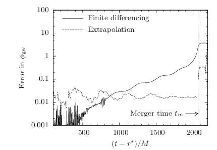
extrapolated to infinite radius. In Fig. 1, we plot the convergence order of . For , we see no clear convergence order, but the differences between the phases at the three resolutions are less than 0.01 radians. For we see a convergence order which drops from 6 to 5, after which the order drops to about 1 for a small period around the merger. The fact that the convergence order is not clearly 6 may be explained by the fact that we have second, fourth and sixth order components in the simulation. Since we do not have clean sixth order convergence, we cannot reliably use Richardson extrapolation to obtain a more accurate result. However, we can use extrapolation of the highest two resolutions using the observed approximate convergence order of 5 to provide an estimate of the error in the solution. Note that for the time region we will use for matching with PN (), the convergence order of 5 is a good approximation. Figure 2 shows the finite differencing error estimate compared with the estimate of the error in the extrapolation to infinite radius. The dotted line represents the time of the peak in , which is a good indicator of the merger time. Note the sudden increase in the extrapolation error shortly after the merger. Also note that any significant effects arising from numerical reflections of the waves from refinement boundaries are expected to be covered by the finite differencing error bars, as these effects should diminish with increased resolution.
When comparing with PN later, we will add the errors from finite differencing and from extrapolation in quadrature to provide an estimate of the overall error in the numerical waveform. Note that the approximately exponential growth of the finite differencing error in Fig. 2 has been previously observed in the circular case [65].


When comparing NR and PN models, we wish to use the gravitational wave frequency . However, as seen before for both finite differencing [13] and pseudo-spectral [15] codes in the circular case, has noticeable high frequency error at early times when the amplitude of the radiation is low. In our case, this comes from numerical reflections of the initial spurious radiation, present in the initial data, from mesh refinement boundaries. Since this is precisely the regime in which we would like to match with PN, this high frequency error must be removed. We find that this can be achieved very effectively by filtering the noisy region of in the Fourier domain. We first tried using a moving averages filter, but this tended to systematically reduce the amplitude of the oscillations in , which we found unacceptable. We also chose not to fit a polynomial to as has been done in the circular case [13], due to the naturally oscillatory nature of the eccentric signal. To perform the filtering, we proceeded as follows. We first chose an interval of time, , in which to perform the filtering. We chose , excluding the late inspiral and merger as well as the initial spurious radiation from the filtering region. We then performed a discrete Fourier transform of the data, removed all but the lowest 30 modes, and then inverse transformed. We found that 30 modes were sufficient to represent the signal; this was judged by subtracting the filtered from the unfiltered signal, and observing essentially only noise. Taking only the first 30 modes corresponds to a frequency cutoff of , or modes with a period of . Note that this is not comparable to filtering the evolved variables or even ; it is the frequency of that is being filtered. Since the original signal is not periodic, Gibbs phenomena were observed as oscillations near the endpoints of the filtered region. We therefore removed a segment of length from the beginning and end of the filtered region before re-inserting the filtered region into the full signal. Fig. 3 shows the result of the filtering.
We have monitored the irreducible masses of the apparent horizons in the lowest resolution simulation. The computed mass of each black hole drops from its initial value of 0.5 by only by the time of the merger, and we ascribe this effect to finite differencing error. We have not computed horizons at higher resolutions due to computational expense. Thus, within our numerical errors, we do not detect any physical growth of the horizons during the inspiral, which potentially could have occurred due to absorption of gravitational wave energy in the initial part of the simulation, as has been studied in detail in previous work [68].
The spins of the black holes, as measured using an approximate technique derived from the isolated horizon formalism [69, 70], increase during the simulation to only before the merger. This is independent of finite differencing resolution, but we expect this tiny spin to be of little consequence to the PN comparison, which does not contain the effects of spin.
The outer boundary in the simulations is at , and as mentioned in Sec.II.2, the boundary condition is a source of error in the simulation. To measure the effect of this error, we have repeated the low resolution simulation, which has only modest computational cost, with the outer boundary moved to by enlarging the coarsest grid. We find that the effect on the waveform phase is much smaller than the estimated errors in the high resolution simulation due to finite differencing and extrapolation to infinite radius, and we conclude that the outer boundary is not a significant source of error in the simulation. In future, with more accurate simulations, this will need to be addressed further.
The simulations at the three different resolutions consumed approximately 5000, 11000 and 16000 CPU hours respectively, each one running on 32 cores of the LoneStar supercomputer.
III.2 Comparing numerical relativity simulations with post-Newtonian models
We now discuss the results of applying the fitting procedure described in Section II.3 to the numerical simulation results.


Figures 4 and 5 show the parameters (for the x model) and (for the n model) determined by fits of the NR data to the PN model in fitting intervals . These parameters are the values of the functions , , , and at . In Fig. 4, has been kept fixed to a value at the start of the usable waveform and has been varied. We see that the parameters obtained from fits using the model vary much less with the fitting window length than those using the model. Specifically, we see that for both models the fitted parameters oscillate significantly for intervals of less than , but for the model these variations die away as the interval is increased beyond this. From the initial data parameters, the orbital period is . It may be that over timescales smaller then the orbital period, there are unmodeled non-adiabatic oscillations in the NR result which are averaged out when larger fitting intervals are used. These oscillations may cause the fit to become worse for small intervals. For the model we see strong oscillations of a period roughly corresponding to the period of the oscillations in itself. In order to determine the effect on the parameters of the interval location, we choose an interval width of and vary in Fig. 5. Here again we see that the model shows much more consistent behavior than the model.
In order to choose a unique set of PN parameters, we choose the earliest possible fitting interval, and take the size of the interval to approximately correspond to the initial orbital period, , giving a fitting interval . The parameters for this fitting interval are given in Table 1. It is interesting to compare these parameters with the approximate parameters used to construct the Bowen-York initial data; these are also given in the table. and agree to within 1% and 2% respectively with the initial data values. agrees within 0.3% between the two PN models, and to 3% with the initial data value. agrees to within 0.1 radians between the two models and the initial data value. agrees to within 0.02 radians between the two models, but is of the order of different from the initial data value. This large discrepancy is probably related to the adjustment of the coordinate system that happens at the start of the numerical simulation. Recall that the method for constructing the initial data parameters was approximate, due to the different coordinate systems used, so perfect agreement is not expected.
| Parameter | -model fit | -model fit | Initial data value |
|---|---|---|---|
| - | |||
| - | |||
Now that we have estimated the PN model which matches the NR solution in the fitting interval, we can compare the PN waveform for the and models with the NR result. In Fig. 6, we plot the PN and NR gravitational wave frequencies and see that there is good agreement with the model from the start of the simulation to . That there is such a high level of agreement with a model which contains so much structure is a strong validation of both the PN model and the NR simulation. We also see on the same plot the much worse agreement obtained using the -model.

We now quantify the agreement with the and -models by considering the waveform phase differences. Fig. 7 shows the difference between the NR and PN gravitational wave phases as a function of . The error bars represent the uncertainty in the NR phase from extrapolation to infinite radius and finite differencing truncation error. We see that the phase difference between NR and PN is within 0.1 radians for approximately , or 11 GW cycles. At , corresponding to , the phase difference between NR and PN is radians.
To put the phase difference of 0.7 radians at into context, we note that the TaylorT4 circular PN model, which is very similar to our eccentric model with , has been shown to have a phase difference at of radians for 2 PN radiation reaction (see Fig. 22 in Ref. [15]). We should be cautious about drawing the conclusion that the agreement in the circular case is better, however, as may not be directly comparable in the two cases, particularly because oscillates in the eccentric case, but is monotonic in the circular case. The steepness of the phase difference in Fig. 22 in Ref. [15] at that point makes the comparison very sensitive to the exact point chosen.

III.3 Choice of post-Newtonian variables
Throughout this work we have presented the results of fitting two PN models with NR data. The two models differ only in the choice of variable used: the frequency-related variable or the mean motion . Our first attempts at matching the NR simulation with an eccentric PN model used . We studied this case extensively, but found significant disagreement, as has been shown. Faced with this disagreement, we studied the (much simpler) circular case using a simulation [25] with low-eccentricity initial data [71] and a circular PN model formed by taking our eccentric -model and setting . This model is suboptimal as it only has 2 PN radiation reaction, and 3.5 PN expressions are available for the circular case. The agreement between NR and PN is very poor even in the circular case using ; the gravitational wave phase difference at is radians. (Note that one should be careful about making direct detailed comparisons between the circular and eccentric cases, due to the ambiguity in the choice of reference point due to the eccentric oscillations in .) However, expressing the PN equations in terms of the coordinate angular velocity of the black holes, , as is common in the literature, gives a significant improvement over using ; at , the phase difference is 0.8 radians. This is in broad agreement with the difference of radians in Fig. 22 of Ref. [15] for the TaylorT4 model at 2 PN, accounting for the uncertainty in the choice of comparison time. This motivated us to search for a frequency-related variable applicable in the eccentric case, and we chose to use , for compatibility with Ref. [49] (recall that in the eccentric case, ), leading to the 0.7 radian phase difference at we report here.
IV Conclusions
We have presented NR results for an inspiraling eccentric black hole binary system with initial eccentricity and compared them with two adiabatic eccentric PN models ( and ) with 2 PN radiation reaction. For the model, the gravitational wave phase agrees to within radians between 21 and 11 cycles before merger. The difference grows to 0.7 radians at cycles before merger (), in broad agreement with the circular case at 2 PN order. One cycle before the merger, the solution to the PN ODEs diverges, indicating a breakdown of the model.
We found that it was necessary to express the PN model in terms of the frequency-related variable rather than the mean motion to get this level of agreement. We conjecture that, when expressed in terms of , certain higher order PN terms are non-negligible, whereas when expressed in terms of , they are small, leading to a smaller error in the PN solution. This can be likened to studies [13, 15] where different circular PN approximants of the same order have been shown to have different errors in the NR regime. In particular, the TaylorT4 circular model showed a remarkable agreement in the waveform phase, but there was a noticeable disagreement in the energy flux [17]. It has also been shown that this remarkable agreement is lost when spinning systems are considered [13]. Our eccentric PN model based on is very similar to TaylorT4 as , so we would expect the same conclusions to apply.
Now that it is possible to match NR and PN eccentric waveforms, we plan to start to construct hybrid templates and begin to assess the implications for the interferometric detection of gravitational wave signals from eccentric binaries close to and including merger. Since complete 3 PN radiation reaction terms for the angular momentum flux have now also been computed, we will be able to compare with a fully 3 PN model, and expect the agreement with NR to get better closer to the merger.
Acknowledgements.
This work was supported in part by NSF grants PHY-0925345 to DS, PHY-0653303, PHY-0555436, PHY-0855892, PHY-0914553 to PL, PHY-0941417, PHY-0903973 to PL and DS, and PHY-0114375 (CGWP). Computations were performed at NCSA and TACC under allocation TG-PHY060013N. Computer algebra and data analysis were performed using Mathematica. The authors thank M. Ansorg, T. Bode, A. Knapp, and E. Schnetter for contributions to the computational infrastructure and E. Bentivegna, J. Read and N. Yunes for helpful discussions.Appendix A PN expressions
We now present, for reference, the full PN expressions used in this work. The expressions for the 3 PN conservative dynamics (i.e. , , , ) can be derived in two ways from the existing literature. They are given directly in Ref. [47] in terms of and , so all that remains is to express them in terms of and . Recall that is defined as where and . In Ref. [48], is used in place of , where . This reference gives expressions for , and in terms of and ; these can be used to obtain in terms of and ,
| (21) | ||||
| (22) | ||||
| (23) | ||||
| (24) |
where, for brevity, we have written . This expression for is then substituted into the conservative expressions in Ref. [47] to obtain the conservative expressions in terms of and , dropping any resulting terms which are higher than 3 PN. Alternatively, we can derive these expressions by taking the expressions for the orbital elements in Ref. [48], along with the expressions for and , all in terms of and . By both methods, we obtain for the separation ,
| (25) | ||||
| (26) | ||||
| (27) | ||||
| (28) | ||||
| (29) |
The relative angular velocity is found to be
| (30) | ||||
| (31) | ||||
| (32) | ||||
| (33) | ||||
| (34) |
The 3 PN Kepler equation is
| (35) | ||||
| (36) | ||||
| (37) | ||||
| (38) |
where, as in Ref. [47], we use
| (39) |
and
| (40) |
is given by
| (41) | ||||
| (42) | ||||
| (43) | ||||
| (44) |
This completes the expressions used in the conservative dynamics. The radiation reaction is given to 2 PN order in Ref. [47] in terms of and . We again substitute for in terms of , and obtain
| (45) | ||||
| (46) | ||||
| (47) | ||||
| (48) |
| (49) |
for , and
| (50) | ||||
| (51) | ||||
| (52) | ||||
| (53) | ||||
| (54) |
for . These equations are written in terms of the functions and , given in Ref. [46] in terms of infinite sums of Bessel functions. We reproduce them here for completeness.
| (55) | ||||
| (56) |
These are functions of only, and are computed numerically using a sufficient number of terms in the summation that the result converges to within machine precision (). For computational efficiency, the resulting function is converted into an interpolating polynomial, and the interpolation error is estimated to be in the range .
References
- [1] B. C. Barish and R. Weiss, Phys. Today 52N10, 44 (1999)
- [2] S. J. Waldmann (LIGO Scientific), Class. Quant. Grav. 23, S653 (2006)
- [3] S. Hild (LIGO Scientific), Class. Quant. Grav. 23, S643 (2006)
- [4] F. Acernese et al. (VIRGO), Class. Quant. Grav. 19, 1421 (2002)
- [5] F. Acernese et al., Class. Quant. Grav. 23, S635 (2006)
- [6] N. Yunes and E. Berti, Phys. Rev. D77, 124006 (2008), arXiv:0803.1853 [gr-qc]
- [7] F. Pretorius, Phys. Rev. Lett. 95, 121101 (Sep. 2005), gr-qc/0507014
- [8] M. Campanelli, C. O. Lousto, P. Marronetti, and Y. Zlochower, Phys. Rev. Lett. 96, 111101 (2006), arXiv:gr-qc/0511048
- [9] J. G. Baker, J. Centrella, D.-I. Choi, M. Koppitz, and J. van Meter, Phys. Rev. Lett. 96, 111102 (2006), arXiv:gr-qc/0511103
- [10] J. G. Baker, J. Centrella, D.-I. Choi, M. Koppitz, and J. van Meter, Phys. Rev. D73, 104002 (2006)
- [11] A. Buonanno, G. B. Cook, and F. Pretorius, Phys. Rev. D 75, 124018 (Jun. 2007), arXiv:gr-qc/0610122
- [12] J. G. Baker, J. R. van Meter, S. T. McWilliams, J. Centrella, and B. J. Kelly, Phys. Rev. Lett. 99, 181101 (2007), arXiv:gr-qc/0612024
- [13] M. Hannam, S. Husa, U. Sperhake, B. Brügmann, and J. A. González, Phys. Rev. D77, 044020 (2008), arXiv:0706.1305 [gr-qc]
- [14] A. Gopakumar, M. Hannam, S. Husa, and B. Bruegmann, Phys. Rev. D78, 064026 (2008), arXiv:0712.3737 [gr-qc]
- [15] M. Boyle et al., Phys. Rev. D76, 124038 (2007), arXiv:0710.0158 [gr-qc]
- [16] T. Damour, A. Nagar, E. N. Dorband, D. Pollney, and L. Rezzolla, Phys. Rev. D77, 084017 (2008), arXiv:0712.3003 [gr-qc]
- [17] M. Boyle et al.(2008), arXiv:0804.4184 [gr-qc]
- [18] E. Berti et al., Phys. Rev. D76, 064034 (2007), arXiv:gr-qc/0703053
- [19] M. Hannam, S. Husa, B. Bruegmann, and A. Gopakumar, Phys. Rev. D78, 104007 (2008), arXiv:0712.3787 [gr-qc]
- [20] P. Ajith et al., Phys. Rev. D77, 104017 (2008), arXiv:0710.2335 [gr-qc]
- [21] P. Ajith, Class. Quant. Grav. 25, 114033 (2008), arXiv:0712.0343 [gr-qc]
- [22] A. Buonanno et al., Phys. Rev. D76, 104049 (2007), arXiv:0706.3732 [gr-qc]
- [23] Y. Pan et al., Phys. Rev. D77, 024014 (2008), arXiv:0704.1964 [gr-qc]
- [24] U. Sperhake et al., Phys. Rev. D78, 064069 (2008), arXiv:0710.3823 [gr-qc]
- [25] I. Hinder, B. Vaishnav, F. Herrmann, D. Shoemaker, and P. Laguna, Phys. Rev. D77, 081502 (2008), arXiv:0710.5167 [gr-qc]
- [26] P. C. Peters, Phys. Rev. 136, B1224 (1964)
- [27] M. Campanelli, C. O. Lousto, and Y. Zlochower, Phys. Rev. D77, 101501 (2008), arXiv:0710.0879 [gr-qc]
- [28] Y. Kozai, Astronomical Journal 67, 591 (Nov. 1962)
- [29] L. Wen, Astrophys. J. 598, 419 (Nov. 2003)
- [30] M. J. Benacquista, Living Rev. Rel. 5, 2 (2002), arXiv:astro-ph/0202056
- [31] K. Gultekin, M. C. Miller, and D. P. Hamilton, Astrophys. J. 616, 221 (2004), arXiv:astro-ph/0402532
- [32] K. S. Thorne and V. B. Braginskii, Astrophys. J. Lett. 204, L1 (Feb. 1976)
- [33] O. Blaes, M. H. Lee, and A. Socrates, Astrophys. J. 578, 775 (2002), arXiv:astro-ph/0203370
- [34] M. Dotti, M. Colpi, and F. Haardt, Mon. Not. R. Astron. Soc. 367, 103 (Mar. 2006)
- [35] P. C. Peters and J. Mathews, Phys. Rev. 131, 435 (Jul 1963)
- [36] R. V. Wagoner and C. M. Will, Astrophys. J. 210, 764 (1976)
- [37] L. Blanchet and G. Schäfer, Mon. Not. R. Astron. Soc. 239, 845 (1989)
- [38] W. Junker and G. Schäfer, Mon. Not. R. Astron. Soc. 254, 146 (Jan. 1992)
- [39] L. Blanchet and G. Schäfer, Class. Quant. Grav. 10, 2699 (1993)
- [40] R. Rieth and G. Schäfer, Class. Quant. Grav. 14, 2357 (1997)
- [41] T. Damour and G. Schäfer, Nuovo Cim. B101, 127 (1988)
- [42] G. Schäfer and N. Wex, Physics Lett. A 174, 196 (1993)
- [43] N. Wex, Classical and Quantum Gravity 12, 983 (Apr. 1995)
- [44] A. Gopakumar and B. R. Iyer, Phys. Rev. D56, 7708 (1997), arXiv:gr-qc/9710075
- [45] A. Gopakumar and B. R. Iyer, Phys. Rev. D65, 084011 (2002), arXiv:gr-qc/0110100
- [46] T. Damour, A. Gopakumar, and B. R. Iyer, Phys. Rev. D70, 064028 (2004), arXiv:gr-qc/0404128
- [47] C. Königsdörffer and A. Gopakumar, Phys. Rev. D 73, 124012 (Jun. 2006)
- [48] R.-M. Memmesheimer, A. Gopakumar, and G. Schäfer, Phys. Rev. D70, 104011 (2004), arXiv:gr-qc/0407049
- [49] K. G. Arun, L. Blanchet, B. R. Iyer, and M. S. S. Qusailah, Phys. Rev. D 77, 064035 (Mar. 2008), arXiv:0711.0302
- [50] K. G. Arun, L. Blanchet, B. R. Iyer, and M. S. S. Qusailah, Phys. Rev. D 77, 064034 (Mar. 2008), arXiv:0711.0250
- [51] K. Arun, Ph.D. thesis, Jawaharlal Nehru University, New Delhi (2006)
- [52] K. G. Arun, L. Blanchet, B. R. Iyer, and S. Sinha, Phys. Rev. D80, 124018 (2009), arXiv:0908.3854 [gr-qc]
- [53] L. Blanchet, Living Reviews in Relativity 9, 4 (Jun. 2006)
- [54] H. Goldstein, C. P. Poole, and J. L. Safko, Classical Mechanics (Addison-Wesley, 2002)
- [55] J. N. Goldberg, A. J. MacFarlane, E. T. Newman, F. Rohrlich, and E. C. G. Sudarshan, J. Math. Phys. 8, 2155 (1967)
- [56] C. M. Will and A. G. Wiseman, Phys. Rev. D 54, 4813 (1996), gr-qc/9608012
- [57] M. Ansorg, B. Brügmann, and W. Tichy, Phys. Rev. D 70, 064011 (2004)
- [58] T. Nakamura, K. Oohara, and Y. Kojima, Prog. Theor. Phys. Suppl. 90, 1 (1987)
- [59] M. Shibata and T. Nakamura, Phys. Rev. D 52, 5428 (1995)
- [60] T. Baumgarte and S. Shapiro, Phys. Rev. D 59, 024007 (1999)
- [61] S. Husa, I. Hinder, and C. Lechner, Computer Physics Communications 174, 983 (Jun. 2006)
- [62] Cactus Computational Toolkit home page, http://www.cactuscode.org/
- [63] E. Schnetter, S. H. Hawley, and I. Hawke, Class. Quant. Grav. 21, 1465 (21 March 2004)
- [64] B. Vaishnav, I. Hinder, F. Herrmann, and D. Shoemaker, Phys. Rev. D 76, 084020 (2007)
- [65] S. Husa, J. A. Gonzalez, M. Hannam, B. Bruegmann, and U. Sperhake, Class. Quant. Grav. 25, 105006 (2008), arXiv:0706.0740 [gr-qc]
- [66] M. Alcubierre, B. Brügmann, P. Diener, M. Koppitz, D. Pollney, E. Seidel, and R. Takahashi, Phys. Rev. D 67, 084023 (2003), gr-qc/0206072
- [67] D. R. Fiske, J. G. Baker, J. R. van Meter, D. Choi, and J. M. Centrella, Phys. Rev. D 71, 104036 (2005), gr-qc/0503100
- [68] T. Bode, D. Shoemaker, F. Herrmann, and I. Hinder, Phys. Rev. D77, 044027 (2008), arXiv:0711.0669 [gr-qc]
- [69] F. Herrmann, I. Hinder, D. M. Shoemaker, P. Laguna, and R. A. Matzner, Phys. Rev. D76, 084032 (2007), arXiv:0706.2541 [gr-qc]
- [70] A. Ashtekar and B. Krishnan, Living Rev. Rel. 7, 10 (2004)
- [71] S. Husa, M. Hannam, J. A. González, U. Sperhake, and B. Brügmann, Phys. Rev. D77, 044037 (2008), arXiv:0706.0904 [gr-qc]