RBC–UKQCD Collaboration

Proton lifetime bounds from chirally symmetric lattice QCD

Preprint: Edinburgh 2008/19, RBRC-728, BNL-HET-08/13

Y. Aoki Affiliation: RIKEN-BNL Research Center, Brookhaven National Laboratory, Upton, NY 11973, USA. P. Boyle Affiliation: SUPA, School of Physics, The University of Edinburgh, Edinburgh EH9 3JZ, UK P. Cooney Affiliation: SUPA, School of Physics, The University of Edinburgh, Edinburgh EH9 3JZ, UK L. Del Debbio Affiliation: SUPA, School of Physics, The University of Edinburgh, Edinburgh EH9 3JZ, UK R. Kenway Affiliation: SUPA, School of Physics, The University of Edinburgh, Edinburgh EH9 3JZ, UK C.M. Maynard Affiliation: EPCC, School of Physics, The University of Edinburgh, Edinburgh EH9 3JZ, UK A. Soni Affiliation: High Energy Theory Group, Brookhaven National Laboratory, Upton, NY 11973, USA R. Tweedie Affiliation: SUPA, School of Physics, The University of Edinburgh, Edinburgh EH9 3JZ, UK RBC–UKQCD Collaboration Affiliation:

August 24, 2026

Abstract

We present results for the matrix elements relevant for proton decay in Grand Unified Theories (GUTs). The calculation is performed at a fixed lattice spacing $a^{-1}=1.73(3)$ GeV using 2+1 flavors of domain wall fermions on lattices of size $16^{3}\times 32$ and $24^{3}\times 64$ with a fifth dimension of length 16. We use the indirect method which relies on an effective field theory description of proton decay, where we need to estimate the low energy constants, $\alpha=-0.0112(25)$ ${\rm{GeV^{3}}}$ and $\beta=0.0120(26)$ ${\rm{GeV^{3}}}$ . We relate these low energy constants to the proton decay matrix elements using leading order chiral perturbation theory. These can then be combined with experimental bounds on the proton lifetime to bound parameters of individual GUTs.

pacs

11.15.Ha, 12.38.-t 12.38.Gc 12.10.Dm

I Introduction

Proton decay is a distinctive experimental signature of Grand Unified Theories (GUTs). Decay experiments can test the predictions of these theories, and, even though direct nucleon decays have not been observed, the experimental lower bound on the decay rate has already ruled out the simplest minimal supersymmetric models [1]. One of the expected decay channels is $N\rightarrow\mathrm{M}+l$ , where $N$ and $\mathrm{M}$ indicate respectively the nucleon and a pseudoscalar meson ( $K,\pi$ ), while $l$ is a lepton ( $e$ , $\mu$ , $\nu_{e}$ , $\nu_{\mu}$ ). This decay is induced by supersymmetric particles or heavy gauge boson exchange, which can be integrated out to obtain an effective Lagrangian describing the low–energy dynamics in terms of the usual Standard Model fields. The lowest–dimensional operators that appear in this approach are $(\bar{q}^{c}q)(\bar{l}^{c}q)$ operators of dimension six; the transition amplitude for the decay is proportional to their hadronic matrix elements $\langle M|(\bar{q}^{c}q)(\bar{l}^{c}q)|N\rangle$ . A quantitative estimate of such hadronic matrix elements, which requires taming non–perturbative QCD effects, is a key ingredient in probing the effects of higher–dimensional operators in GUTs models at current experiments.

Several determinations of the hadronic matrix elements have been performed in the past [2, 3, 4, 5, 6, 7, 8, 9, 10, 11, 12, 13, 14, 15], using either QCD bound state phenomenological models, or lattice QCD. Due to recent progress in simulating dynamical fermions, lattice QCD has become a quantitative method to compute hadronic matrix elements from first principles with controlled systematic uncertainties. The matrix elements relevant for nucleon decay can be extracted from three-point correlators computed on the lattice. This is the so–called direct method, which requires an expensive computer simulation. However, the same matrix elements can also be computed, at the cost of introducing difficult to estimate systematics, using the chiral lagrangian describing proton decay [16]: in this case they are expressed as functions of the low–energy constants (LECs) that appear in the chiral lagrangian. These LECs can be computed from two–point lattice correlators at a lesser computational cost. However, such an indirect determination of the matrix elements depends on the accuracy of chiral perturbation theory, and therefore is affected by an additional source of systematic error.

In this work, we present a new determination of the matrix elements that are relevant for nucleon decay based on the indirect method, using dynamical Domain Wall Fermion (DWF) configurations with $2+1$ flavours. Our results extend the ones obtained for $2$ flavours of dynamical DWF in Ref. [15]. Systematic errors are greatly reduced by simulating at light quark masses, and using non–perturbative renormalization. Note that the exponentially suppressed chiral symmetry breaking of DWF greatly simplifies the mixing of operators under renormalization, which improves the precision of the final result. The correct number of flavours gives confidence in setting the scale, a large source of uncertainty in some early lattice determinations.

The chiral perturbation theory results used for this work are summarized in Section II, which also sets the notation used throughout the paper. The chiral Lagrangian for nucleon decay involves two LECs, which are obtained by extrapolating to the chiral limit the outcome of numerical simulations performed at light quark masses. A direct measurement of the hadronic matrix element using lattice three–point functions, which relies much less on the validity of chiral perturbation theory, is in progress, and is deferred to a subsequent publication.

Details of our lattice simulations are reported in Section III. Our results are obtained from gauge configurations with volumes of $16^{3}\times 32$ and $24^{3}\times 64$ . Both have a fifth dimension of size $L_{s}=16$ and use the Iwasaki gauge action. The lattice spacing is $a\approx 0.114~\mathrm{fm}$ corresponding to physical volumes of $(1.8~\mathrm{fm})^{3}$ , and $(2.7~\mathrm{fm})^{3}$ respectively. Being able to compare two different physical volumes enables us to estimate the finite volume effects. Results for meson spectroscopy and topology have already been presented in Ref. [17] for the smaller lattice and in Ref. [18] for the larger lattice. We refer to these publication for details of calculations involving the lattices which are used in this paper. The range of fermion masses simulated for this work yields a ratio of the pseudoscalar to vector meson masses in the range $0.378\leq m_{\mathrm{PS}}/m_{\mathrm{V}}\leq 0.615$ . Working at fixed lattice spacing, we are not able to present a continuum extrapolation for our final result. Nonetheless, it should be noted that DWFs are automatically O(a) improved ¹¹ 1 Due to finite $L_{s}$ there are small $\mathcal{O}(a)$ errors, which, however are negligible compared to the other errors in this study, and is therefore expected to have a good scaling behavior.

Section IV presents our results for the non–perturbative renormalization (NPR) of the three–quark operators, using the RI–MOM scheme. We compute the renormalization mixing matrix and perform the matching required to obtain the renormalized operators in the $\overline{\mathrm{MS}}$ -scheme.

In the last Section of the paper, we combine the lattice amplitudes with the renormalization factors to compute the phenomenologically relevant matrix elements in the $\overline{\mathrm{MS}}$ scheme. We discuss the error budget in detail including estimates of the systematic error due to the chiral extrapolation, the renormalization, the finite volume and the choice of method to set the lattice spacing, and the foreseeable improvements on the current estimate.

II Chiral lagrangian for proton decay

Integrating out the heavy GUT particles yields the low–energy effective Lagrangian describing nucleon decay written in terms of the QCD fundamental fields:

{\mathcal{L}}^{\Delta B}=\sum_{d=1,2}\sum_{i=1}^{4}C^{(i)}_{d}Q^{(i)}_{d}+\sum_{d=1,2}\sum_{i=1}^{6}\tilde{C}^{(i)}_{d}\tilde{Q}^{(i)}_{d},

(1)

where $d$ denotes the generation of the lepton produced in the decay, and $i$ is a label for the dimension–six operators containing three quark and one lepton field that describe nucleon decay. $C^{(i)}_{d}$ and $\tilde{C}^{(i)}_{d}$ are Wilson coefficients. The full list of operators $Q^{(i)}$ , $\tilde{Q}^{(i)}$ was identified on symmetry grounds in Refs. [19, 20, 21]; their matrix elements between hadronic states determine the decay amplitude. For instance, the matrix elements that are relevant for the process where a proton decays into a pion are:

\langle\pi(\vec{p})|\epsilon_{abc}(u^{aT}CP_{R,L}d^{b})P_{L}u^{c}|p(\vec{k},s)\rangle=P_{L}\left[W_{0}^{R/LL}(q^{2})-i/\!\!\!qW_{q}^{R/LL}(q^{2})\right]u(k,s),

(2)

where $a,b,c$ are colour indices, $C$ is the charge-conjugation operator, and $P_{R,L}=\frac{1\pm\gamma_{5}}{2}$ are the right– and left–handed projectors. The non–perturbative dynamical effects are captured by the two form factors that appear on the RHS of Eq. (2), while $q$ (the momentum carried by the electron) is the momentum transfer. It is convenient to introduce here a generic notation for three–quark operators with an arbitrary spin structure:

\mathcal{O}^{\Gamma\Gamma^{\prime}}(\vec{x},t)=\epsilon_{abc}\left[u^{a}(\vec{x},t)(C\Gamma)d^{b}(\vec{x},t)\right]\Gamma^{\prime}u^{c}(\vec{x},t).

(3)

where $\Gamma$ and $\Gamma^{\prime}$ are elements of the Clifford algebra in four–dimensional Euclidean spacetime, and we have omitted spinor indices. We use the notation $S=1$ , $P=\gamma_{5}$ , $V=\gamma_{\mu}$ , $A=\gamma_{\mu}\gamma_{5}$ , $T=\sigma_{\mu\nu}=\frac{1}{2}\{\gamma_{\mu},\gamma_{\nu}\}$ , $R=P_{R}$ , and $L=P_{L}$ . Further operators with this structure appear when computing the nucleon mass, and upon renormalization, as discussed in Sects. III, and IV.

Following the notation in Refs. [16, 13], the chiral Lagrangian describing baryon–meson dynamics is written in terms of a pseudoscalar meson (octet) field:

\phi=\left(\begin{array}[]{ccc}\sqrt{\frac{1}{2}}\pi^{0}+\sqrt{\frac{1}{6}}\eta&\pi^{+}&K^{+}\\ \pi^{-}&-\sqrt{\frac{1}{2}}\pi^{0}+\sqrt{\frac{1}{6}}\eta&K^{0}\\ K^{-}&\bar{K}^{0}&-\sqrt{\frac{2}{3}}\eta\\ \end{array}\right),

(4)

and a spinor baryon (octet) field:

B=\left(\begin{array}[]{ccc}\sqrt{\frac{1}{2}}\Sigma^{0}+\sqrt{\frac{1}{6}}\Lambda^{0}&\Sigma^{+}&p\\ \Sigma^{-}&-\sqrt{\frac{1}{2}}\Sigma^{0}+\sqrt{\frac{1}{6}}\Lambda^{0}&n\\ \Xi^{-}&\Xi^{0}&-\sqrt{\frac{2}{3}}\Lambda^{0}\\ \end{array}\right).

(5)

At lowest order in powers of momentum, and in Euclidean space-time, the chirally symmetric Lagrangian is written as:

$\displaystyle{\mathcal{L}}_{0}=$	$\displaystyle\frac{f^{2}}{8}\mathrm{Tr}(\partial_{\mu}\Sigma)(\partial_{\mu}\Sigma^{\dagger})+\mathrm{Tr}\bar{B}(\gamma_{\mu}\partial_{\mu}+M_{B})B$
	$\displaystyle+\frac{1}{2}\mathrm{Tr}\bar{B}\gamma_{\mu}\left[\xi\partial_{\mu}\xi^{\dagger}+\xi^{\dagger}\partial_{\mu}\xi\right]B+\frac{1}{2}\mathrm{Tr}\bar{B}\gamma_{\mu}B\left[\left(\partial_{\mu}\xi\right)\xi^{\dagger}+\left(\partial_{\mu}\xi^{\dagger}\right)\xi\right]$
	$\displaystyle-\frac{1}{2}(D-F)\mathrm{Tr}\bar{B}\gamma_{\mu}\gamma_{5}B\left[\left(\partial_{\mu}\xi\right)\xi^{\dagger}-\left(\partial_{\mu}\xi^{\dagger}\right)\xi\right]$
	$\displaystyle+\frac{1}{2}(D+F)\mathrm{Tr}\bar{B}\gamma_{\mu}\gamma_{5}\left[\xi\partial_{\mu}\xi^{\dagger}-\xi^{\dagger}\partial_{\mu}\xi\right]B,$	(6)

where the unitary matrices $\Sigma$ and $\xi$ are defined as:

\Sigma=\exp\left(\frac{2i\phi}{f}\right),~~~~~\xi=\exp\left(\frac{i\phi}{f}\right).

(7)

Introducing a diagonal quark mass matrix:

M=\left(\begin{array}[]{ccc}m_{u}&&\\ &m_{d}&\\ &&m_{s}\end{array}\right),

(8)

the symmetry–breaking part of the chiral Lagrangian becomes:

	$\displaystyle{\mathcal{L}}_{1}=$	$\displaystyle-v^{3}\mathrm{Tr}\left(\Sigma^{\dagger}M+M\Sigma\right)-a_{1}\mathrm{Tr}\bar{B}\left(\xi^{\dagger}M\xi^{\dagger}+\xi M\xi\right)B-a_{2}\mathrm{Tr}\bar{B}B\left(\xi^{\dagger}M\xi^{\dagger}+\xi M\xi\right)$
		$\displaystyle-b_{1}\mathrm{Tr}\bar{B}\gamma_{5}\left(\xi^{\dagger}M\xi^{\dagger}-\xi M\xi\right)B-b_{2}\mathrm{Tr}\bar{B}\gamma_{5}B\left(\xi^{\dagger}M\xi^{\dagger}-\xi M\xi\right).$		(9)

The low–energy constants that appear in the chiral Lagrangian are extracted from phenomenological analyses. In particular, following the notation in Ref. [16], $f$ is the pion decay constant in the chiral limit, 130(5) MeV [22]. The combination $F+D$ yields the nucleon axial charge, $g_{A}=1.2695(29)$ [22], while the combination $F-D$ is related to the ratio of the zero–momentum form factors for semileptonic hyperon decay, $g_{1}/f_{1}$ [23]. Together these give, $F=0.47(1)$ and $D=0.80(1)$ . $a_{1}$ and $a_{2}$ are symmetry–breaking parameters, but their values are not required in this work. The parameters $b_{1}$ , $b_{2}$ are not precisely determined and are an extra source of systematic error.

The transformation properties under SU(3) ${}_{L}\times$ SU(3)_R of the three-quark operators in Eq. 1 determine the expression of the baryon–number violating operators in the chiral Lagrangian. The latter appear in the Lagrangian with two new low–energy constants $\alpha$ and $\beta$ [16]:

$\displaystyle{\mathcal{L}}^{\Delta B}=$	$\displaystyle\alpha\sum_{d=1}^{2}\left\{C_{d}^{(1)}\left[e_{dL}\mathrm{Tr}{\mathcal{F}}\xi B_{L}\xi-\nu_{dL}\mathrm{Tr}{\mathcal{F}}^{\prime}\xi B_{L}\xi\right]\right.$
	$\displaystyle+C_{d}^{(2)}e_{dR}\mathrm{Tr}{\mathcal{F}}\xi^{\dagger}B_{R}\xi^{\dagger}+\tilde{C}_{d}^{(1)}\left[e_{dL}\mathrm{Tr}\tilde{{\mathcal{F}}}\xi B_{L}\xi-\nu_{dL}\mathrm{Tr}\tilde{{\mathcal{F}}}^{\prime}\xi B_{L}\xi\right]$
	$\displaystyle\left.+\tilde{C}_{d}^{(2)}e_{dR}\mathrm{Tr}\tilde{{\mathcal{F}}}\xi^{\dagger}B_{R}\xi^{\dagger}+\tilde{C}_{d}^{(5)}\nu_{dL}\mathrm{Tr}\tilde{{\mathcal{F}}}^{\prime\prime}\xi B_{L}\xi\right\}+$
	$\displaystyle\beta\sum_{d=1}^{2}\left\{C_{d}^{(3)}\left[e_{dL}\mathrm{Tr}{\mathcal{F}}\xi B_{L}\xi^{\dagger}-\nu_{dL}\mathrm{Tr}{\mathcal{F}}^{\prime}\xi B_{L}\xi^{\dagger}\right]\right.$
	$\displaystyle+C_{d}^{(4)}e_{dR}\mathrm{Tr}{\mathcal{F}}\xi^{\dagger}B_{R}\xi+\tilde{C}_{d}^{(3)}\left[e_{dL}\mathrm{Tr}\tilde{{\mathcal{F}}}\xi B_{L}\xi^{\dagger}-\nu_{dL}\mathrm{Tr}\tilde{{\mathcal{F}}}^{\prime}\xi B_{L}\xi^{\dagger}\right]$
	$\displaystyle\left.+\tilde{C}_{d}^{(4)}e_{dR}\mathrm{Tr}\tilde{{\mathcal{F}}}\xi^{\dagger}B_{R}\xi+\tilde{C}_{d}^{(6)}\nu_{dL}\mathrm{Tr}\tilde{{\mathcal{F}}}^{\prime\prime}\xi B_{L}\xi^{\dagger}\right\}+{\rm{h.c.}}$	(10)

The matrices ${\mathcal{F}},{\mathcal{F}}^{\prime},\tilde{{\mathcal{F}}},\tilde{{\mathcal{F}}}^{\prime}$ , and $\tilde{{\mathcal{F}}}^{\prime\prime}$ are projectors in flavour space; their explicit expressions are:

{\mathcal{F}}=\left(\begin{array}[]{ccc}0&0&0\\ 0&0&0\\ 1&0&0\end{array}\right),{\mathcal{F}}^{\prime}=\left(\begin{array}[]{ccc}0&0&0\\ 0&0&0\\ 0&1&0\end{array}\right),\tilde{{\mathcal{F}}}=-\left(\begin{array}[]{ccc}0&0&0\\ 1&0&0\\ 0&0&0\end{array}\right),\tilde{{\mathcal{F}}}^{\prime}=-\left(\begin{array}[]{ccc}0&0&0\\ 0&1&0\\ 0&0&0\end{array}\right),\tilde{{\mathcal{F}}}^{\prime\prime}=\left(\begin{array}[]{ccc}0&0&0\\ 0&0&0\\ 0&0&1\end{array}\right).

(11)

Eqs. 10 and 11 show that the low–energy constants $\alpha$ and $\beta$ determine the matrix elements:

	$\displaystyle\langle 0\|\mathcal{O}^{RL}\|p({\mathbf{k}},s)\rangle=$	$\displaystyle\alpha\ P_{L}u({\mathbf{k}},s)$		(12)
	$\displaystyle\langle 0\|\mathcal{O}^{LL}\|p({\mathbf{k}},s)\rangle=$	$\displaystyle\beta\ P_{L}u({\mathbf{k}},s)$		(13)

where $u({\mathbf{k}},s)$ is the spinor associated with a proton of momentum ${\mathbf{k}}$ and spin projection $s$ . The phase definition is fixed such that $\alpha$ and $\beta$ are real and $\alpha<0$ . As we will later describe, we observe $\alpha+\beta\simeq 0$ , which is expected because of the relation,

(\alpha+\beta)\ u({\mathbf{k}},s)=-\langle 0|\epsilon^{abc}(u^{Ta}Cd^{b})\gamma_{5}u^{c}|p({\mathbf{k}},s)\rangle,

(14)

which vanishes in the non-relativistic limit and is known to be quite small even at small quark masses [24].

Using chiral perturbation theory to compute the matrix element in Eq. (2) yields for the $N\rightarrow\pi$ transition [16, 13]:

$\displaystyle\langle\pi^{0}\|\mathcal{O}^{RL}\|p({\mathbf{k}},s)\rangle$	$\displaystyle=$	$\displaystyle\alpha P_{L}u({\mathbf{k}},s)\left[\frac{1}{\sqrt{2}f}-\frac{D+F}{\sqrt{2}f}\frac{-q^{2}+m_{N}^{2}}{-q^{2}-m_{N}^{2}}-\frac{4b_{1}}{\sqrt{2}f}\frac{m_{u}m_{N}}{-q^{2}-m_{N}^{2}}\right]$	(15)
	$\displaystyle-$	$\displaystyle\alpha P_{L}iq\!\!\!\!\;/\penalty u({\mathbf{k}},s)\left[\frac{D+F}{\sqrt{2}f}\frac{2m_{N}}{-q^{2}-m_{N}^{2}}+\frac{4b_{1}}{\sqrt{2}f}\frac{m_{u}}{-q^{2}-m_{N}^{2}}\right],$	(15)
$\displaystyle\langle\pi^{0}\|\mathcal{O}^{LL}\|p({\mathbf{k}},s)\rangle$	$\displaystyle=$	$\displaystyle\beta P_{L}u({\mathbf{k}},s)\left[\frac{1}{\sqrt{2}f}-\frac{D+F}{\sqrt{2}f}\frac{-q^{2}+m_{N}^{2}}{-q^{2}-m_{N}^{2}}-\frac{4b_{1}}{\sqrt{2}f}\frac{m_{u}m_{N}}{-q^{2}-m_{N}^{2}}\right]$	(16)
	$\displaystyle-$	$\displaystyle\beta P_{L}iq\!\!\!\!\;/\penalty u({\mathbf{k}},s)\left[\frac{D+F}{\sqrt{2}f}\frac{2m_{N}}{-q^{2}-m_{N}^{2}}+\frac{4b_{1}}{\sqrt{2}f}\frac{m_{u}}{-q^{2}-m_{N}^{2}}\right],$	(16)

where $q$ is the four-momentum of the outgoing lepton. In the limit where $q^{2}\ll m_{N}^{2}$ and $b_{1}m_{u}\ll m_{N}$ , these expressions simplify to:

	$\displaystyle\langle\pi^{0}\|\mathcal{O}^{RL}\|p({\mathbf{k}},s)\rangle$	$\displaystyle\simeq$	$\displaystyle\alpha P_{L}u({\mathbf{k}},s)\left[\frac{1}{\sqrt{2}f}+\frac{D+F}{\sqrt{2}f}\right]+O(m_{l}^{2}/m_{N}^{2}),$		(17)
	$\displaystyle\langle\pi^{0}\|\mathcal{O}^{LL}\|p({\mathbf{k}},s)\rangle$	$\displaystyle\simeq$	$\displaystyle\beta P_{L}u({\mathbf{k}},s)\left[\frac{1}{\sqrt{2}f}+\frac{D+F}{\sqrt{2}f}\right]+O(m_{l}^{2}/m_{N}^{2}),$		(18)

where $-q^{2}=m_{l}^{2}$ is the on–shell condition for the outgoing lepton. The equations above relate the proton decay matrix elements to the low–energy constants $\alpha$ and $\beta$ ; note that, in order to reconstruct the matrix elements on the lhs of Eqs. 17 and 18 using the indirect method, the combination $F+D$ and the pion decay constant, $f$ , are also required.

III Lattice simulations

III.1 Dataset description

The analysis was performed on 2+1 flavor DWF ensembles with volumes of $16^{3}\times 32$ and $24^{3}\times 64$ generated using the Iwasaki gauge action with $\beta=2.13$ and the domain wall fermion quark action with $L_{s}=16$ . At each volume we generated sets of configurations with a light isodoublet with masses $am_{ud}$ = 0.005 ( $24^{3}\times 64$ only), 0.01, 0.02 or 0.03 and a fixed approximate strange quark mass, $am_{s}=0.04$ . The ensembles, described in [25] and [18], have a fixed inverse lattice spacing of $a^{-1}=1.73(3)$ GeV and were generated with the RHMC algorithm with a trajectory length of $\tau=1$ . These same datasets were used to calculate $g_{A}$ , [26]. The configurations used for both the non–perturbative renormalisation and the matrix element calculation are shown in Table 1.

		Matrix Elements					NPR
$V\times L_{s}$	$am_{ud}$	$N_{\rm{traj}}$	$\Delta$	$N_{\rm{cfg}}$	$N_{\rm{src}}$	$N_{\rm{bin}}$	$N_{\rm{traj}}$	$\Delta$	$N_{\rm{cfg}}$	$N_{\rm{src}}$	$N_{\rm{bin}}$
	0.01	500-4000	10	175	4	8	1000-4000	40	75	4	1
$16^{3}\times 32\times 16$	0.02	500-4000	10	175	4	8	1000-4000	40	75	4	1
	0.03	500-7580	10	177	2	8	1000-4000	40	75	4	1
	0.005	900-4500	10	90	2	8
			10	90	$2\times 2$	8
$24^{3}\times 64\times 16$	0.01	1500-3860	10	59	2	8
			40	59	2	2
	0.02	1800-3600	10	45	2	8
			40	45	2	2
	0.03	1020-3060	20	51	1	2
			40	51	1	1

Table 1: RHMC 2+1 flavour datasets used for the non-perturbative renormalization and matrix element calculation.

V

is the space-time volume of the lattice,

L_{s}

is the extent of the fifth dimension,

am_{ud}

is the up sea quark mass (the strange sea quark mass is kept fixed at 0.04),

N_{\rm{traj}}

is the lowest to highest trajectories analysed with matrix elements calculated every

\Delta

trajectories,

N_{\rm{cfg}}

is the number of configurations,

N_{\rm{src}}

is the number of quark propagators solved with different source locations and

N_{\rm{bin}}

is the bin size.

24^{3}\times 64\times 16

data were generated for the non-perturbative renormalization calculation, however, it was only used as a check for finite volume errors and so does not appear here. For the

24^{3}\times 64\times 16

matrix element data, there are two independent runs for each of the sea quark masses. These independent runs used different smearings,

\Delta

, source locations and

N_{\rm{src}}

For each of the seven ensembles matrix elements were calculated using correlation functions composed of valence quarks with masses equal to the light quark mass in the sea. To improve statistics, correlators were oversampled and averaged into bins whose size depended on the Monte Carlo time separation between measurements. The binning was consistent with the integrated auto-correlation length for the pseudoscalar meson correlators at the time separation typically used, which was calculated to be of order 50 trajectories. Multiple sources per configuration and several different types of smearing have also been used to improve the signal. As well as local sources ( $L$ ), we employ gauge–invariant Gaussian smearing with two different smearing radii ( $G$ and $G*$ ) and gauge fixed hydrogen–like wavefunction smearing ( $H$ ). One or both of the propagators used to construct the two-point correlators for mesons may be smeared while for baryons, one, two or all three propagators may be smeared. We adopt the same convention used in Ref. [27] for naming the smeared two–point functions.

The chiral limit is defined as the value of $am_{f}$ such that $am_{f}+am_{\mathrm{res}}=0$ , where $am_{\mathrm{res}}=0.00315(2)$ is the residual quark mass, estimated in Refs. [27, 28, 25]. The lattice scale is determined from a combination of the $\Omega^{-}$ baryon mass and the pseudoscalar kaon and pion masses, yielding a value $a^{-1}=1.729(28)$ GeV (see Ref. [18] for details).

The parameters used in the simulations correspond to a pseudoscalar meson mass ranging from $331$ MeV to $671$ MeV. The renormalization constant for the axial current, $Z_{A}=0.7162(2)$ , which we will use in the non-perturbative renormalization of the nucleon decay operators, was obtained from a hadronic matrix element of the conserved DWF axial current in Ref. [28].

III.2 Nucleon mass and amplitude

Starting from the correlator of two operators, $\mathcal{O}^{\Gamma_{1}\Gamma_{2}}$ and $\mathcal{O}^{\Gamma_{3}\Gamma_{4}}$ , we can define the scalar two–point function:

f_{\Gamma_{1}\Gamma_{2},\Gamma_{3}\Gamma_{4}}(t)=\sum_{\vec{x}}\mathrm{Tr}\ \left[\langle\mathcal{O}^{\Gamma_{1},\Gamma_{2}}(\vec{x},t)\overline{\mathcal{O}}^{\Gamma_{3},\Gamma_{4}}(0)\rangle\left(\frac{1+\gamma_{4}}{2}\right)\right].

(19)

Using the notation introduced so far, $\mathcal{O}^{PS}(\vec{x},t)$ is the usual local proton interpolating operator:

\mathcal{O}^{PS}(\vec{x},t)=\epsilon_{abc}\left[u^{aT}(\vec{x},t)C\gamma_{5}d^{b}(\vec{x},t)\right]u^{c}(\vec{x},t),

(20)

and the large–time exponential fall–off of the correlator $f_{PS,PS}$ is dictated by the nucleon mass:

f_{PS,PS}(t)=2e^{-am_{N}t}G_{N}^{2}+\ldots,

(21)

where $G_{N}$ is the overlap of the proton interpolating field to the normalized proton state:

\langle 0|\mathcal{O}^{PS}(\vec{0},0)|p({\mathbf{k}},s)\rangle=G_{N}u({\mathbf{k}},s).

(22)

The nucleon mass is obtained from the two–point functions $f_{PS,PS}(t)$ and $f_{A_{4}S,A_{4}S}(t)$ , each of them being computed for several smearing combinations. Firstly, for each two–point function and for each smearing combination, we calculate the effective mass:

m_{N,\mathrm{eff}}(t)=\log\left[\frac{f(t)}{f(t+1)}\right]

(23)

where $f(t)$ indicates the two–point function in any one of the channels used for the analysis. Results for the effective mass computed from both two–point functions, and for two different smearing combinations, are reported in Fig. 1. The agreement between the different channels within the error bars is clearly seen in the first plot on the left for the $24^{3}\times 64$ data with $am_{u}=0.01$ . The effective mass can be fitted to the same constant $m$ for each channel; correlations between different time–slices are taken into account by minimizing a correlated $\chi^{2}$ :

\chi^{(n)2}(m^{(n)})=\sum_{t,t^{\prime}}\left[m^{(n)}_{N,\mathrm{eff}}(t)-m^{(n)}\right]C^{(n)-1}_{tt^{\prime}}\left[m^{(n)}_{N,\mathrm{eff}}(t^{\prime})-m^{(n)}\right]

(24)

where $C^{(n)}_{tt^{\prime}}$ is the covariance matrix:

C^{(n)}_{tt^{\prime}}=\frac{1}{N_{\mathrm{boot}}}\sum_{m=1}^{N_{\mathrm{boot}}}\left[\bar{m}_{N,\mathrm{eff}}^{(n,m)}(t)-\langle\bar{m}_{N,\mathrm{eff}}^{(n)}(t)\rangle\right]\left[\bar{m}_{N,\mathrm{eff}}^{(n,m)}(t^{\prime})-\langle\bar{m}_{N,\mathrm{eff}}^{(n)}(t^{\prime})\rangle\right]

(25)

the index $n$ represents a bootstrap resampling of the original data, and the index $m$ represents a bootstrap resampling of the $n^{\mathrm{th}}$ bootsample. ${N_{\mathrm{boot}}}$ is the number of bootstrap samples, $\bar{m}_{N,\mathrm{eff}}^{(n,m)}(t)$ is the effective mass determined from the $m^{\mathrm{th}}$ resampling of the $n^{\mathrm{th}}$ bootsample and $\langle\bar{m}_{N,\mathrm{eff}}^{(n)}(t)\rangle$ is the average of the effective mass over the $m^{\mathrm{th}}$ resampling of the $n^{\mathrm{th}}$ bootsample.

Refer to caption — Figure 1: (a) is an effective mass plot and (b) is an effective amplitude (Eq.26) plot for the nucleon. Both are calculated on the $24^{3}\times 64$ dataset with $am_{u}=0.01$ . The different colours in the effective mass plot correspond to different smearings. Datasets are labelled with the smearing (i.e. LL). Those datasets labelled with a 2 use the operator $f_{A_{4}S,A_{4}S}(t)$ , the rest use $f_{PS,PS}(t)$ . (c) is a linear extrapolation of the ground state mass to the chiral limit.

All channels display a plateau for the effective mass, and the limiting values are compatible within the statistical errors. The smeared propagators reach the limiting value earlier, as expected, thus yielding a longer plateau for the fit to be performed. In order to increase the precision of the fit, all channels were fitted simultaneously to a single constant $m$ ; correlations between different channels are also taken into account in the construction of the covariance matrix. Note that with this fitting procedure several channels are fitted simultaneously without adding extra parameters, and the minimization in the one–dimensional parameter space can be performed analytically.

The fit to the amplitude, $G_{N}$ , is subsequently performed by defining an effective amplitude:

G^{2}_{N,\mathrm{eff}}(t)=\frac{1}{2}f_{PS,PS}(t)\exp(mt),

(26)

where $m$ is the nucleon mass obtained in the fit described above, and we used the same notation as in Eq. 23 to denote the two-point function. $G_{N}$ is then obtained from a fit to a constant by minimizing a fully correlated $\chi^{2}$ , as discussed above for the nucleon mass. Results for $G_{N,\mathrm{eff}}(t)$ are displayed in Fig. 1(b), where a long plateau is clearly visible.

For all the fits presented here, the results of the minimization procedure are stable with respect to sensible variations of the fit range. All the correlators, smearings, and fit ranges are summarized in Table 2. Variations of the fitted parameters remain within their statistical error as the bounds of the fitting range are shifted by $\pm 1$ timeslice.

For the case of the nucleon mass on the $am_{u}=0.005$ , $V=24^{3}\times 64$ ensemble (the ensemble with the lightest valence quark mass), there was some difficulty in judging exactly where the plateau for the effective mass started. Fitting to different time ranges gave incompatible results. To account for this, we performed a fit over a large time range, spanning the multiple potential plateaux. The incompatibility of the data was reflected in a poor value of $\chi^{2}$ per degree of freedom (d.o.f) of 4.3. In order to deal with this we rescaled the errors on all the points in the effective mass plot by $\sqrt{\chi^{2}/\mathrm{d.o.f}}$ and performed a second fit to this rescaled data. This gave a $\chi^{2}$ /d.o.f of 1, as expected, and a fitted mass compatible with the best fit value from before, but with a larger error. The fits to the effective mass on this ensemble before and after rescaling are shown in Fig. 2.

The nucleon mass and amplitude are extrapolated linearly to the chiral limit. The result of the extrapolation for the nucleon mass on the $24^{3}\times 64$ dataset is displayed in Fig. 1(c). The results for the nucleon masses obtained from the fits are summarized in Table 3.

	$V=16^{3}\times 32$						$V=24^{3}\times 64$
$m_{u}$			Fit Range						Fit Range
	Smearing	$O^{\Gamma\Gamma}$	$m_{N}$	$G_{N}$	$\alpha$	$\beta$	Smearing	$O^{\Gamma\Gamma}$	$m_{N}$	$G_{N}$	$\alpha$	$\beta$
0.005							LL	$O^{PS}$	-	9-12	5-8	5-9
							HL	$O^{PS}$	6-12	-	4-10	4-9
							HL	$O^{A_{4}S}$	6-12	-	-	-
							G*L	$O^{PS}$	6-12	-	-	-
							GG	$O^{PS}$	6-12	-	-	-
0.01	LL	$O^{PS}$	9-12	9-12	5-8	5-8	LL	$O^{PS}$	9-12	9-12	7-11	5-10
	LL	$O^{A_{4}S}$	9-12	-	-	-	LL	$O^{A_{4}S}$	9-12	-	-	-
	GL	$O^{PS}$	9-12	-	3-8	3-8	GL	$O^{PS}$	8-12	-	7-11	4-10
	GL	$O^{A_{4}S}$	9-12	-	-	-	GL	$O^{A_{4}S}$	8-12	-	-	-
							G*L	$O^{PS}$	7-12	-	-	-
0.02	LL	$O^{PS}$	9-12	9-12	6-12	5-12	LL	$O^{PS}$	9-10	9-12	7-11	5-10
	LL	$O^{A_{4}S}$	9-12	-	-	-	LL	$O^{A_{4}S}$	9-10	-	-	-
	GL	$O^{PS}$	8-12	-	6-10	4-14	HL	$O^{PS}$	9-11	-	7-11	7-10
	GL	$O^{A_{4}S}$	8-12	-	-	-	HL	$O^{A_{4}S}$	9-11	-	-	-
	GG	$O^{PS}$	8-11	-	-	-	G*L	$O^{PS}$	9-11	-	-	-
	GG	$O^{A_{4}S}$	8-11	-	-	-
0.03	LL	$O^{PS}$	10-12	9-12	7-11	6-11	LL	$O^{PS}$	10-12	9-12	9-13	9-11
	LL	$O^{A_{4}S}$	10-12	-	-	-	LL	$O^{A_{4}S}$	10-12	-	-	-
	GL	$O^{PS}$	8-12	-	7-11	8-12	HL	$O^{PS}$	9-12	-	9-13	9-11
	GL	$O^{A_{4}S}$	8-12	-	-	-	HL	$O^{A_{4}S}$	9-12	-	-	-
	GG	$O^{PS}$	8-12	-	-	-	G*L	$O^{PS}$	8-12	-	-	-
	GG	$O^{A_{4}S}$	8-12	-	-	-

Table 2: Smearings, operators and fit ranges used for the calculation of nucleon masses, nucleon amplitudes and matrix elements.

III.3 Low–energy constants

As discussed in the previous section, the low–energy parameters $\alpha$ and $\beta$ appearing in the chiral Lagrangian can be calculated at leading order through the proton to vacuum matrix elements:

\displaystyle\langle 0|{\mathcal{O}}^{RL}|p({\mathbf{k}},s)\rangle=\alpha P_{L}u({\mathbf{k}},s),

\displaystyle\langle 0|{\mathcal{O}}^{LL}|p({\mathbf{k}},s)\rangle=\beta P_{L}u({\mathbf{k}},s),

(27)

\displaystyle-\langle 0|{\mathcal{O}}^{LR}|p({\mathbf{k}},s)\rangle=\alpha P_{R}u({\mathbf{k}},s),

\displaystyle-\langle 0|{\mathcal{O}}^{RR}|p({\mathbf{k}},s)\rangle=\beta P_{R}u({\mathbf{k}},s),

(28)

where Eq. 28 is obtained from Eq. 27 by parity transformation. The low–energy constants are obtained from the asymptotic behaviour of ratios of two–point functions for large Euclidean time $t$ :

	$\displaystyle R_{\alpha}(t)$	$\displaystyle=$	$\displaystyle 2G_{N}\frac{f_{RL,PS}(t)}{f_{PS,PS}(t)}\rightarrow\alpha,$		(29)
	$\displaystyle R_{\beta}(t)$	$\displaystyle=$	$\displaystyle 2G_{N}\frac{f_{LL,PS}(t)}{f_{PS,PS}(t)}\rightarrow\beta.$		(30)

A typical plateau obtained for $R_{\alpha}$ is shown in Fig. 3. Two different smearing combinations were used in the analysis, which correspond respectively to a local and a smeared interpolating field $\mathcal{O}^{PS}(\vec{x},t)$ for the nucleon. They both yield consistent results, as shown in the plot. The values of the low–energy constants were obtained by fitting the data to a constant, for each value of the quark masses. As for the spectrum, $\chi^{2}$ is always defined taking into account the correlation between different time-slices. The results obtained from the fits are given in Table 3.

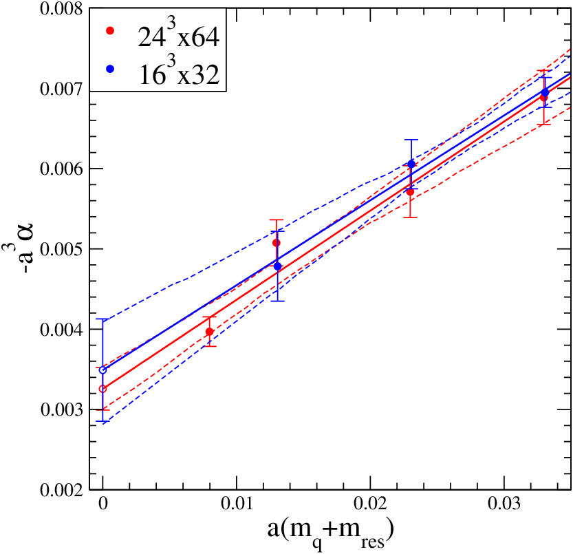
The data points are extrapolated linearly to the chiral limit, as shown in Fig. 4. The data in the mass range studied in this work appear to be consistent with a linear behaviour, leading to a good fit for the chiral extrapolation. An uncorrelated $\chi^{2}$ is used in this case, since the points at different values of the quark mass are produced by independent runs.

$V\times L_{s}$	$am_{ud}/am_{s}$	$am_{N}$	$a^{3}\alpha$	$a^{3}\beta$
	0.03/0.04	0.908(6)	-0.00695(19)	$0.00719(21)$
$16^{3}\times 32\times 16$	0.02/0.04	0.819(8)	-0.00605(31)	$0.00606(30)$
	0.01/0.04	0.722(19)	-0.00478(43)	$0.00511(47)$
	chiral		-0.00349(64)	$0.00369(63)$
	0.03/0.04	0.892(10)	-0.00689(33)	$0.00621(38)$
$24^{3}\times 64\times 16$	0.02/0.04	0.805(12)	-0.00571(32)	$0.00598(38)$
	0.01/0.04	0.720(10)	-0.00508(29)	$0.00486(28)$
	0.005/0.04	0.671(5)	-0.00397(18)	$0.00400(22)$
	chiral		-0.00326(27)	$0.00348(32)$

Table 3: Results from fits described in this paper. The nucleon masses the LECs

\alpha

and

\beta

are reported as a function of the quark masses, for both lattices used in this study. The results of linear chiral extrapolations are also reported in the last line of each column. All the results are given in units of the lattice spacing

a\approx 0.12~\mathrm{fm}

IV Non–perturbative renormalization

IV.1 RI–MOM mixing matrix

For the non–perturbative renormalisation of the proton decay matrix elements we employ the non–perturbative, MOM-scheme, renormalisation technique of the Rome-Southampton group [29] as used by [15],[29] and [30]. The application of this technique to proton decay matrix elements is outlined in [15] which we briefly summarise.

The operators, $\mathcal{O}^{\Gamma\Gamma^{\prime}}$ , can be classified according to their symmetry properties under parity ( $\mathcal{P}$ ) and the so-called switching transformation ( $\mathcal{S}$ ). The result of such classification is summarized in Table 4.

	$\mathcal{S}^{-}$	$\mathcal{S}^{+}$
$\mathcal{P}^{-}$	$SS$ , $PP$ , $AA$	$VV$ , $TT$
$\mathcal{P}^{+}$	$SP$ , $PS$ , $-AV$	$-VA$ , $T\tilde{T}$

Table 4: Classification of the

\mathcal{O}^{\Gamma\Gamma^{\prime}}

operators according to their transformation properties under parity and switching.

In the presence of chiral symmetry breaking, operators that belong to the same sector mix under renormalisation. Concentrating on the $\mathcal{S}^{-}$ sectors, the renormalised operators in the parity basis are defined as:

\mathcal{O}^{A}_{ren}=\tilde{Z}^{AB}_{\mathrm{ND}}\mathcal{O}^{B}_{latt},\quad A,B=\{SS,PP,AA\},

(31)

where $A$ and $B$ label the possible choices for $\Gamma\Gamma^{\prime}$ and $\tilde{Z}^{AB}_{\mathrm{ND}}$ is a $3\times 3$ mixing matrix. The same mixing matrix renormalizes the operators in the sector $\mathcal{P}^{-}$ and $\mathcal{P}^{+}$ . The chirality basis, which contains the operators of interest for the nucleon decay matrix elements, consists of

$\displaystyle LL$	$\displaystyle=$	$\displaystyle\frac{1}{4}(SS+PP)-\frac{1}{4}(SP+PS)$	(32)
$\displaystyle RL$	$\displaystyle=$	$\displaystyle\frac{1}{4}(SS-PP)-\frac{1}{4}(SP-PS)$	(33)
$\displaystyle A(LV)$	$\displaystyle=$	$\displaystyle\frac{1}{2}AA-\frac{1}{2}(-AV),$	(34)

hence, the mixing matrix in the chirality basis, $Z_{\mathrm{ND}}$ , and in the parity basis are related via:

Z_{\mathrm{ND}}=\mathcal{T}\tilde{Z}_{\mathrm{ND}}\mathcal{T}^{-1},

(35)

where

\mathcal{T}=\left(\begin{array}[]{ccc}1/4&1/4&0\\ 1/4&-1/4&0\\ 0&0&1/2\end{array}\right).

(36)

The mixing matrix in the parity basis is computed from the non–perturbative amputated three–quark vertex function of the operators in the $\mathcal{S}^{-}$ sector as a function of external leg momentum $p$ after gauge fixing to Landau gauge. The number of configurations used in the non–perturbative renormalisation is given in Table 1. The vertex function is defined as the amputated Fourier transform of the correlator of $\mathcal{O}^{A}$ with three quark spinors:

\mathcal{G}^{A}(p^{2})_{abc\;\alpha\beta\;\gamma\delta}=\epsilon^{a^{\prime}b^{\prime}c^{\prime}}(C\Gamma)_{\alpha^{\prime}\beta^{\prime}}\Gamma^{\prime}_{\delta\gamma^{\prime}}\langle Q_{\alpha^{\prime}\alpha}^{a^{\prime}a}(p)Q_{\beta^{\prime}\beta}^{b^{\prime}b}(p)Q_{\gamma^{\prime}\gamma}^{c^{\prime}c}(p)\rangle,

(37)

where

Q_{\alpha^{\prime}\alpha}^{a^{\prime}a}(p)=\langle S^{a^{\prime}a^{\prime\prime}}_{\alpha^{\prime}\alpha^{\prime\prime}}(p)\rangle^{-1}S_{\alpha^{\prime\prime}\alpha}^{a^{\prime\prime}a}(p),\quad S_{\alpha^{\prime}\alpha}^{a^{\prime}a}(p)=\int dx\,e^{-ip.x}\,S_{\alpha^{\prime}\alpha}^{a^{\prime}a}(x),

(38)

$S(x)$ is the quark propagator, and $\Gamma,\Gamma^{\prime}$ are the matrices that appear in $\mathcal{O}^{A}$ .

Introducing the mixing matrix:

M^{AB}(p^{2})=\mathcal{G}^{A}_{abc\;\alpha\beta\;\gamma\delta}\cdot P^{B}_{abc\;\beta\alpha\;\delta\gamma},

(39)

the renormalisation condition in the RI–MOM scheme reads:

Z_{q}^{-3/2}\tilde{Z}_{\mathrm{ND}}^{BC}M^{CA}=\delta^{BA}

(40)

where $Z_{q}$ is the quark wavefunction renormalisation; $a,b,c$ are colour indices and $\alpha$ , $\beta$ , $\gamma$ and $\delta$ are spin indices associated with $\Gamma$ , $\Gamma^{\prime}$ respectively. The projection operators,

$\displaystyle P^{SS}$	$\displaystyle=$	$\displaystyle\frac{1}{96}\epsilon^{abc}(C^{-1})^{\beta\alpha}\delta^{\delta\gamma}$	(41)
$\displaystyle P^{PP}$	$\displaystyle=$	$\displaystyle\frac{1}{96}\epsilon^{abc}(\gamma_{5}C^{-1})^{\beta\alpha}\gamma_{5}^{\delta\gamma}$	(42)
$\displaystyle P^{AA}$	$\displaystyle=$	$\displaystyle\frac{1}{384}\epsilon^{abc}(\gamma_{5}\gamma_{\mu}C^{-1})^{\beta\alpha}(\gamma_{5}\gamma_{\mu})^{\delta\gamma},$	(43)

are chosen such that the renormalisation condition in Eq. 40 is satisfied in the free field case: $Z_{q}=1$ , $Z_{\mathrm{ND}}^{BC}=\delta^{BC}$ .

Fig. 5 shows the mixing matrix, $M^{AB}$ , in the chirality basis as a function of external leg momentum. The set of momenta used to calculate the mixing matrix is defined by

\displaystyle p=\left(\frac{2\pi}{L_{x}}n_{x},\frac{2\pi}{L_{y}}n_{y},\frac{2\pi}{L_{z}}n_{z},\frac{2\pi}{L_{t}}n_{t}\right)

(44)

where $L_{x}=L_{y}=L_{z}$ is the spatial size of the lattice and $L_{t}$ is the time extent. Combinations of $(n_{x},n_{y},n_{z},n_{t})$ such that $-2\leq n_{x},n_{y},n_{z}\leq 2$ and $-4\leq n_{t}\leq 4$ are chosen and then averaged into equal $p^{2}$ values.

Operator mixing is induced by chiral symmetry breaking. The extent to which chiral symmetry is broken in the domain wall action is parameterised by the residual mass, $am_{\rm{res}}$ , and the induced mixing is expected to be suppressed by a factor $(am_{\mathrm{res}})^{2}$ [31]. It may be seen from Fig. 5 that, in the window of momenta for which contributions from both hadronic effects (low momenta) and contributions from discretisation effects (high momenta) are small, the chiral symmetry afforded by the domain wall fermions suppresses the mixing between different chirality operators and results in a mixing matrix which is essentially diagonal. This greatly simplifies the calculation of the proton decay matrix elements compared to, for example, Wilson fermions [13].

The matrix $\tilde{Z}_{\mathrm{ND}}$ can be obtained from the relation $M=Z_{q}^{3/2}\tilde{Z}_{\mathrm{ND}}^{-1}$ , as shown in Eq. 40, which requires $Z_{q}$ to be computed. Instead, we remove the $Z_{q}$ dependence, and exploit the accurate determination of $Z_{A}=0.7162(2)$ at the chiral limit, which was computed from ratios of hadronic matrix elements in Ref. [17], together with the average of the amputated local axial vector and vector bilinear currents, which allows the evaluation of the factor $\Lambda^{A}=Z_{q}/Z_{A}$ . Fig. 6 shows the average and difference of the amputated local axial vector and vector bilinear currents. The non-zero difference may be taken as a measure of the systematic error of the renormalisation constant arising from the closing of the window where the RI–MOM NPR can be safely applied. It may be observed that for $(ap)^{2}\geq 1.7$ there is $<1$ % effect, which is enhanced to $2$ % by extrapolation of $(ap)^{2}\rightarrow 0$ .

The product $\left(\Lambda^{A}\right)^{-3/2}M^{-1}$ yields $\tilde{Z}_{\mathrm{ND}}/Z_{A}^{3/2}$ for each value of the sea quark mass, without having to deal directly with $Z_{q}$ . At finite lattice spacing, $Z_{A}$ ’s only scale dependence is due to the discretisation error, which starts at $O(a^{2}p^{2})$ . Finally the rotation to the chirality basis and a linear chiral extrapolation are performed, the latter may be done very precisely, as the mass dependence is extremely mild, as shown in Fig. 5. As an example, the $p^{2}$ dependence of the $LL$ element of the matrix $Z_{\mathrm{ND}}/Z_{A}^{3/2}$ is displayed in Fig. 6.

IV.2 Scheme matching and RG running

In order to relate the lattice, MOM-scheme, matrix elements at scale $p$ to those in the $\overline{\mathrm{MS}}$ , NDR scheme at some scale $\mu$ we compute the factor

U^{\overline{\mathrm{MS}}\leftarrow latt}(\mu)=U^{\overline{\mathrm{MS}}}(\mu;p)\frac{Z^{\overline{\mathrm{MS}}}(p)}{Z^{MOM}(p)}Z_{\mathrm{ND}}(p),

(45)

where $Z^{\overline{\mathrm{MS}}}(p)/Z^{MOM}(p)$ is the matching factor from $\overline{\mathrm{MS}}$ scheme to MOM scheme at a scale $p$ calculated using continuum perturbation theory, and $U^{\overline{\mathrm{MS}}}(\mu;p)$ is the renormalization group evolution factor from scale $p$ to $\mu$ in the $\overline{\mathrm{MS}}$ scheme. The matching factor has been computed in Ref. [15]:

\frac{Z^{\overline{\mathrm{MS}}}}{Z^{MOM}}=1+\frac{\alpha_{s}}{4\pi}\left[\frac{433}{180}-\frac{1123}{90}\mathop{\rm ln}2+\xi\left(\frac{587}{180}-\frac{317}{90}\mathop{\rm ln}2\right)\right],

(46)

where $\xi=0$ as we work in Landau gauge. The $\overline{\mathrm{MS}}$ evolution factor reads

$\displaystyle U^{\overline{\mathrm{MS}}}(\mu;p)$	$\displaystyle=$	$\displaystyle\left[\frac{\alpha_{s}(\mu)}{\alpha_{s}(p)}\right]^{\gamma_{0}/2\beta_{0}}\left[1+\left(\frac{\gamma_{1}}{2\beta_{0}}-\frac{\beta_{1}\gamma_{0}}{2\beta_{0}^{2}}\right)\frac{\alpha_{s}(\mu)-\alpha_{s}(p)}{4\pi}\right],$	(47)
$\displaystyle\beta_{0}$	$\displaystyle=$	$\displaystyle 11-\frac{2}{3}N_{f},\;\beta_{1}=102-\frac{38}{3}N_{f},$	(48)
$\displaystyle\gamma_{0}$	$\displaystyle=$	$\displaystyle-4,\;\gamma_{1}=-\left(\frac{14}{3}+\frac{4}{9}N_{f}-4\Delta\right),$	(49)

where the anomalous dimension of the nucleon decay operator has been calculated up to two loops in $\overline{\mathrm{MS}}$ , NDR scheme [32] and $\Delta=0,-10/3$ for $LL,RL$ operators respectively. The value of $\alpha_{s}(p)$ is obtained by integrating numerically the four–loop $\beta$ function of Ref. [33], starting from $\alpha_{s}(M_{Z})=0.1176(2)$ [22], and matching the value of $\alpha_{s}$ across the $b$ , and $c$ thresholds.

The $\overline{\mathrm{MS}}$ renormalisation factor, Eq. 45, at a fixed scale $\mu=1/a$ is plotted in Fig. 6 as a function of the square of the scale at which the lattice, MOM-scheme, renormalisation calculation was performed. The remaining momentum dependence, due to $O(a^{2}p^{2})$ discretisation errors, is removed by performing a linear extrapolation in $(ap)^{2}$ to $(ap)^{2}=0$ , which is also shown in Fig. 6. This extraploation is performed over the range $1.7<(ap)^{2}<2.5$ where the non-perturbative effect, estimated at $2$ %, is expected to be small.

Together with the value of $Z_{A}$ from the hadronic matrix element ratio and using Eq. 47 to run from $\mu=1/a$ to $\mu=2$ GeV we obtain:

	$\displaystyle U^{\overline{\mathrm{MS}}\leftarrow latt}(\mu=2~\rm{GeV})_{LL}$	$\displaystyle=$	$\displaystyle 0.662\pm 0.010$
	$\displaystyle U^{\overline{\mathrm{MS}}\leftarrow latt}(\mu=2~\rm{GeV})_{RL}$	$\displaystyle=$	$\displaystyle 0.665\pm 0.008$

where the error is statistical.

V Discussion

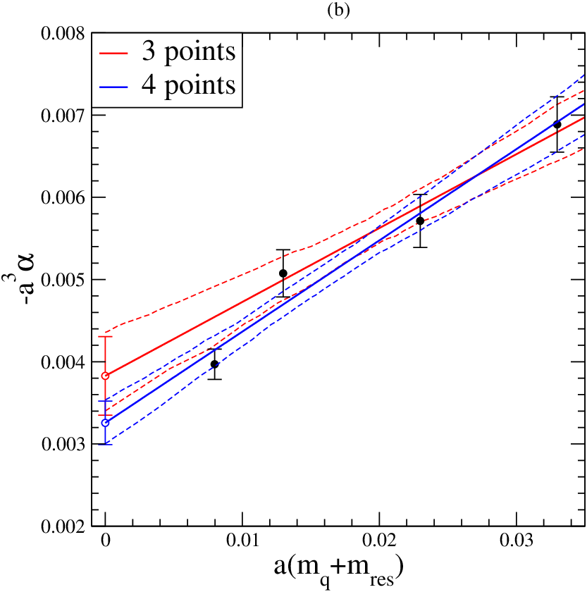
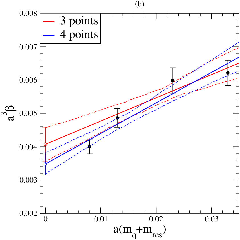
The errors on all quantities so far have been purely statistical. From the results in Table 3 we can see that for this matrix element and for the statistics available, there are no significant finite volume effects as the results on both volumes agree within errors. Fig. 7 shows the agreement for $\alpha$ between the two volumes. As discussed in Section III.2, there is an additional systematic error in calculating the nucleon mass on the ensemble with the lightest valence quark mass ( $am_{u}=0.005$ ). For a conservative analysis we performed an extrapolation for $\alpha$ and $\beta$ both with and without this lightest point. This gave a result which differed by 18% for $\alpha$ and 17% for $\beta$ as shown in Fig. 8. We use this as an estimate of the error in extrapolating to the chiral limit.

It should be noted that in our simulation, the strange quark mass is held fixed and hence in the extrapolation, only the light quarks are taken to the chiral limit. However, if we compare our result with the $N_{f}=2$ result from [15] we see there is very good agreement (see Fig. 9). For $N_{f}=2$ , the strange quark mass is effectively infinite, the agreement signifies that $\alpha$ and $\beta$ have little dependence on the strange sea quark mass.

For the NPR, we estimate a systematic error of $8$ % which is dominated by the error from truncating the perturbative expansion for the matching factor at order $\alpha_{s}^{2}$ in Eq. 46.

Adding all of these uncertainties in quadrature, and together with the values for the matrix elements in Table 3, we estimate the low–energy parameters renormalised at $\mu=2$ GeV to be:

	$\displaystyle\alpha$	$\displaystyle=$	$\displaystyle-0.0112\pm 0.0012_{(\mathrm{stat})}\pm 0.0022_{(\mathrm{syst})}~\mathrm{GeV}^{3}$		(50)
	$\displaystyle\beta$	$\displaystyle=$	$\displaystyle 0.0120\pm 0.0013_{(\mathrm{stat})}\pm 0.0023_{(\mathrm{syst})}~\mathrm{GeV}^{3}.$		(51)

The results for various determinations of $\alpha$ are summarized in Fig. 9. The agreement between recent lattice computations suggests that lattice QCD is being successful at determining the low-energy constants describing nucleon decay with increasingly smaller systematic uncertainty.

The indirect computation of the proton lifetime has a further non-linear systematic error, due to the use of chiral perturbation theory in a kinematic regime where the pion has a large momentum. The relevant matrix element has been computed using both the indirect and direct methods in Ref. [15] where sizeable differences were seen between the two methods. For the case of the matrix elements in Eq. 17 and 18, the indirect method was found to give an estimate for the matrix element of about two times larger than the direct method.

|\alpha|

[GeV³]

|\beta|

[GeV³]

Donoghue and Goldwich [4]

0.003

Bag model

Thomas and McKellar [7]

0.02

Bag model

Meljanac et al. [5]

0.004

Bag model

QCD model

Ioffe [2]

0.009

Sum rule

calculation

Krasnikov et al. [6]

0.003

Sum rule

Ioffe and Smilga [8]

0.006

Sum rule

Tomozawa [3]

0.006

Quark model

Brodsky et al. [9]

0.03

Hara et al. [10]

0.03

WF,

a=0.11

Bowler et al. [11]

0.013

0.010

WF,

a=0.22

Lattice QCD

Gavela et al. [12]

0.0056(8)

\simeq|\alpha|

WF,

a=0.09

N_{f}=0

JLQCD [13]

0.015(1)

0.014(1)

WF,

a=0.09

CP-PACS & JLQCD [14]

0.0090(09)(

{}^{+5}_{-19}

)

0.0096(09)(

{}^{+6}_{-20}

)

WF, continuum limit

Aoki et al. [15]

0.0100(19)

0.0108(21)

DWF,

a=0.15

Lattice QCD

N_{f}=2

Aoki et al. [15]

0.0118(21)

DWF,

a=0.12

Lattice QCD

N_{f}=2+1

This work

0.0112(25)

0.0120(26)

DWF,

a=0.12

Table 5: Comparison of the low energy parameter of the nucleon decay chiral Lagrangian

\alpha

and

\beta

among various QCD model calculation, lattice results in the literatures and the results from this work. In lattice QCD calculations, WF and DWF mean Wilson and domain-wall fermions. The results for

N_{f}=2

, and our results for

N_{f}=2+1

are shown with the total error consisting of statistical and systematic errors on the bare matrix element and renormalization constant. The errors on the results from

N_{f}=0

are only statistical.

Finally, let us discuss one way to use our result to discriminate between GUTs. The proton partial decay width in a generic channel can be split into

\Gamma=\mathrm{LEC}^{2}\times A_{\mathrm{QCD}}\times A_{\mathrm{GUT}},

(52)

where LEC is the low–energy constant, $\alpha$ or $\beta$ , that we calculate earlier in this paper, $A_{\mathrm{QCD}}$ contains information from QCD parameters and $A_{\mathrm{GUT}}$ contains all the information about the underlying high–energy theory, including constants from the GUT. For the Minimal SUSY SU(5) GUT, expressions for the lifetime have been calculated for several decay modes in Ref. [34].

Dimensional Analysis gives the value of the proton lifetime as $\Gamma_{N}\sim\alpha_{\mathrm{GUT}}^{2}m_{p}^{5}/M_{\mathrm{GUT}}^{4}$ . Taking $M_{\mathrm{GUT}}\approx 10^{16}$ [22] and obtaining $\alpha_{\mathrm{GUT}}$ by running the strong coupling up to the GUT scale gives $\Gamma_{N}\sim 10^{-68}$ GeV. The natural scale for $A_{\mathrm{GUT}}$ is $M_{\mathrm{GUT}}^{-4}$ . The values of the low–energy constant that we have computed, together with the values of the quantities in $A_{\mathrm{QCD}}$ [22] and the experimental bounds on the proton life time [35, 36], allow us to put bounds on $A_{\mathrm{GUT}}$ for different decay modes as summarized in Table 6. The bounds quoted are at a 68% confidence level. The different decay modes provide more or less stringent bounds on $A_{\mathrm{GUT}}$ . The viability of any GUT can be assessed by checking wether the relevant bounds are satisfied.

Decay Mode		Lifetime bound(yrs)	$A_{\mathrm{GUT}}$ bound $(M_{\mathrm{GUT}}^{-4})$
$p\rightarrow$	$e^{+}\pi^{0}$	$>8.2\times 10^{33}$	$<44$
$p\rightarrow$	$e^{+}\pi^{0}$	$>8.2\times 10^{33}$	$<37$
$p\rightarrow$	$K^{+}\bar{\nu}$	$>2.3\times 10^{33}$	$<76$
$n\rightarrow$	$K^{0}\bar{\nu}$	$>1.3\times 10^{32}$	$<733$

Table 6: The experimental proton partial lifetime bounds at

90\%

CL from [35, 36] and the bound on

A_{\mathrm{GUT}}

at a 68% CL that this lifetime bound implies. This bound is given in units of

M_{\mathrm{GUT}}^{-4}

, the numbers quoted in the table are therefore dimensionless. The first line is for a decay mediated by a heavy gauge boson, the second and subsequent lines are for decays mediated by a colour triplet Higgs.

As a simple example, for the decay mode $p\rightarrow e^{+}\pi^{0}$ via X boson exchange in the minimal SU(5) SUSY GUT, $A_{\mathrm{GUT}}(p\rightarrow e^{+}\pi^{0})$ is given by [37] to be

A_{\mathrm{GUT}}(p\rightarrow e^{+}\pi^{0})=\frac{g_{5}^{4}A_{R}^{2}}{M_{X}^{4}}\left|1+\left(1+|V_{ud}|^{2}\right)^{2}\right|

(53)

where $g_{5}$ is the unified coupling at the GUT scale, $M_{X}$ is the mass of the X boson $\approx M_{GUT}$ , $A_{R}$ is the renormalization factor and $V_{ud}$ a CKM matrix element. Using the value of $A_{R}$ given in [37], we can put a bound on the $X$ boson mass of $M_{X}>5\times 10^{15}\mathrm{GeV}$ .

The decay widths of the channels involving colour triplet Higgs exchange can be calculated and involve the LEC $\beta$ (see Ref. [34]). The analysis in Ref. [1] uses a conservative choice of $\beta=0.003\mathrm{GeV}^{3}$ at a scale of 1 GeV to constrain the mass of the colour triplet Higgs sufficiently to rule out the minimal SUSY SU(5) GUT. The higher value calculated in this work (running our value of $\beta$ to a scale of 1 GeV gives $\beta=0.0109\pm 23~\mathrm{GeV}^{3}$ if we use Eq. 47) gives an even stronger constaint on the mass of the colour triplet Higgs and so confirms the fact that the minimal SUSY SU(5) GUT has been ruled out.

The uncertainty on $\alpha^{2}$ is $45\%$ and on $\beta^{2}$ is $43\%$ . These are higher than the uncertainties on the factors $A_{\mathrm{QCD}}$ which for all channels is $\approx 8\%$ . A factor of $\approx 2$ reduction in the uncertainty of the LECs would make them comparable with the uncertainties of $A_{\mathrm{QCD}}$ , which is dominated by the uncertainties of $D$ , $F$ and $f_{\pi}$ . As $M_{X}\sim\sqrt{\alpha}$ , an error of $45\%$ on $\alpha^{2}$ corresponds to an error of $11\%$ on the bound for $M_{X}$ . Reducing the uncertainty on $\alpha$ by a factor of two would therefore reduce the uncertainty from $\alpha$ on the bound for $M_{X}$ to $6\%$ .

Acknowledgments

The calculations reported here were done on the QCDOC computers [38, 39, 40] at Columbia University, Edinburgh University, and at Brookhaven National Laboratory (BNL). At BNL, the QCDOC computers of the RIKEN-BNL Research Center and the USQCD Collaboration were used. The software used includes: the CPS QCD codes http://qcdoc.phys.columbia.edu/chulwoo_index.html, supported in part by the USDOE SciDAC program; the BAGEL http://www.ph.ed.ac.uk/˜paboyle/bagel/Bagel.html assembler kernel generator for many of the high-performance optimized kernels; and the UKHadron codes.

AS (BNL) was partially supported by the U.S. DOE under contract DE-AC02-98CH10886. The work of the Edinburgh authors was supported by PPARC grants PP/D000238/1 and PP/C503154/1. The former directly supported CMM. PAB acknowledges support from RCUK and LDD is funded through an STFC advanced fellowship. The Edinburgh QCDOC system was funded by PPARC JIF grant PPA/J/S/1998/00756 and operated through support from the Universities of Edinburgh, Southampton and Wales Swansea, and from STFC grant PP/E006965/1.-

Computations for this work were carried out in part on facilities of the USQCD Collaboration, which are funded by the Office of Science of the U.S. Department of Energy. We thank RIKEN, BNL and the U.S. DOE for providing the facilities essential for the completion of this work.

We thank Masato Shiozawa for communicating the latest Super-Kamiokande results.

References

[1] H. Murayama and A. Pierce, Phys. Rev. D65, 055009 (2002), eprint hep-ph/0108104.
[2] B. L. Ioffe, Nucl. Phys. B188, 317 (1981).
[3] Y. Tomozawa, Phys. Rev. Lett. 46, 463 (1981).
[4] J. F. Donoghue and E. Golowich, Phys. Rev. D26, 3092 (1982).
[5] S. Meljanac, D. Palle, I. Picek, and D. Tadic, Nucl. Phys. B206, 298 (1982).
[6] N. V. Krasnikov, A. A. Pivovarov, and N. N. Tavkhelidze, JETP Lett. 36, 333 (1982).
[7] A. W. Thomas and B. H. J. Mckellar, Nucl. Phys. B227, 206 (1983).
[8] B. L. Ioffe and A. V. Smilga, Nucl. Phys. B232, 109 (1984).
[9] S. J. Brodsky, J. R. Ellis, J. S. Hagelin, and C. T. Sachrajda, Nucl. Phys. B238, 561 (1984).
[10] Y. Hara, S. Itoh, Y. Iwasaki, and T. Yoshie, Phys. Rev. D34, 3399 (1986).
[11] K. C. Bowler, D. Daniel, T. D. Kieu, D. G. Richards, and C. J. Scott, Nucl. Phys. B296, 431 (1988).
[12] M. B. Gavela et al., Nucl. Phys. B312, 269 (1989).
[13] S. Aoki et al. (JLQCD), Phys. Rev. D62, 014506 (2000), eprint hep-lat/9911026.
[14] N. Tsutsui et al. (CP-PACS), Phys. Rev. D70, 111501 (2004), eprint hep-lat/0402026.
[15] Y. Aoki, C. Dawson, J. Noaki, and A. Soni, Phys. Rev. D75, 014507 (2007a), eprint hep-lat/0607002.
[16] M. Claudson, M. B. Wise, and L. J. Hall, Nucl. Phys. B195, 297 (1982).
[17] D. J. Antonio et al. (2007), eprint hep-lat/0702026.
[18] C. Allton et al. (2008), eprint 0804.0473.
[19] S. Weinberg, Phys. Rev. Lett. 43, 1566 (1979).
[20] F. Wilczek and A. Zee, Phys. Rev. Lett. 43, 1571 (1979).
[21] L. F. Abbott and M. B. Wise, Phys. Rev. D22, 2208 (1980).
[22] W.-M. Yao, C. Amsler, D. Asner, R. Barnett, J. Beringer, P. Burchat, C. Carone, C. Caso, O. Dahl, G. D’Ambrosio, et al., Journal of Physics G 33, 1+ (2006), URL http://pdg.lbl.gov.
[23] S. Y. Hsueh et al., Phys. Rev. D38, 2056 (1988).
[24] S. Sasaki, T. Blum, and S. Ohta, Phys. Rev. D65, 074503 (2002), eprint hep-lat/0102010.
[25] C. Allton et al. (RBC) (2007), eprint hep-lat/0701013.
[26] T. Yamazaki et al. (RBC+UKQCD), Phys. Rev. Lett. 100, 171602 (2008), eprint 0801.4016.
[27] D. J. Antonio et al. (2006), eprint hep-lat/0612005.
[28] C. Allton et al. (UKQCD) (2006), eprint hep-lat/0610119.
[29] G. Martinelli, C. Pittori, C. T. Sachrajda, M. Testa, and A. Vladikas, Nucl. Phys. B445, 81 (1995), eprint hep-lat/9411010.
[30] Y. Aoki et al. (2007b), eprint 0712.1061.
[31] T. Blum et al., Phys. Rev. D66, 014504 (2002), eprint hep-lat/0102005.
[32] T. Nihei and J. Arafune, Prog. Theor. Phys. 93, 665 (1995), eprint hep-ph/9412325.
[33] T. van Ritbergen, J. A. M. Vermaseren, and S. A. Larin, Phys. Lett. B400, 379 (1997), eprint hep-ph/9701390.
[34] J. Hisano, H. Murayama, and T. Yanagida, Nucl. Phys. B402, 46 (1993), eprint hep-ph/9207279.
[35] N. Z. Poster presented by H. Nishino [Super-Kamiokande Collaboration] at Neutrino 08, Christchurch (2008).
[36] K. Kobayashi et al. (Super-Kamiokande), Phys. Rev. D72, 052007 (2005), eprint hep-ex/0502026.
[37] J. Hisano (2000), eprint hep-ph/0004266.
[38] P. Boyle et al., IBM Journal of Research and Development 49, number 2/3, 351 (2005a).
[39] P. A. Boyle, C. Jung, and T. Wettig (QCDOC), ECONF C0303241, THIT003 (2003), eprint hep-lat/0306023.
[40] P. A. Boyle et al., J. Phys. Conf. Ser. 16, 129 (2005b).