Theory of spin current in chiral helimagnet

The core problem in the multidisciplinary field of spintronics is how to create, transport, and manipulate spin currents.[1] The key notions include the current-driven spin-transfer torque[2, 3, 4, 5, 6] and resultant force acting on a domain wall (DW)[7, 8] in metallic ferromagnetic/nonmagnetic multilayers, the dissipationless spin currents in paramagnetic spin-orbit coupled systems,[9, 10, 11] and magnon transport in textured magnetic structures.[12] A fundamental query behind the issue is how to describe transport spin currents.[13] To make clear the meaning of the spin currents, we need to note the spin can appear in the macroscopic Maxwell equations only in the form of spin magnetization. In this viewpoint, the spin current is understood as the deviation of the spin projection from its equilibrium value. An emergence of the coherent collective transport in non-equilibrium state is then a manifestation of the dynamical off-diagonal long range order (DODLRO).[14, 15]

On the other hand, the physical currents are classified into two categories, i.e., the gauge current originating from the gauge invariance and the inertial current originating from the Galilean invariance. The electric current is the gauge current, where the electric charge is coupled to the electromagnetic U(1) gauge field. The electromagnetic field is a physical gauge field that has its own dynamics, i.e., we know the electromagnetic field energy. Then, the charge current $j_{i}$ and the charge density $\rho$ are related via the continuity equation $\partial\rho/\partial t=-\partial j_{i}/\partial x_{i}$. On the other hand, a typical example of the inertial current is the momentum current in a classical ideal fluid, where the momentum current $\Pi_{ij}$ satisfies the continuity equation, $\partial\left(\rho v_{i}\right)/\partial t=-\partial\Pi_{ij}/\partial x_{j},$ and given by $\Pi_{ij}=P\delta_{ij}+\rho v_{i}v_{j}$ with $P$ being equilibrium pressure.[16] The non-equilibrium current is described by $\rho v_{i}v_{j}$. In the spin current problem, at present, we have no known gauge field directly coupled to the spin current. Therefore, a promising candidate is the inertial current of the magnetization.

Historically, Döring[17] pointed out that the longitudinal component of the slanted magnetic moment inside the Bloch DW emerges as a consequence of translational motion of the DW. An additional magnetic energy associated with the resultant demagnetization field is interpreted as the kinetic energy of the wall. This idea was simplified by Becker[18] and Kittel.[19] Recent progress of material synthesis sheds new light on this problem. In a series of magnets belonging to chiral space group without any rotoinversion symmetry elements, the crystallographic chirality gives rise to the asymmetric Dzyaloshinskii interaction that stabilizes either left-handed or right-handed chiral magnetic structures.[20] In these chiral helimagnets, magnetic field applied perpendicular to the helical axis stabilizes a periodic array of DWs with definite spin chirality forming kink crystal or chiral soliton lattice.[21]

We recently proposed a new way to generate a spin current in the chiral helimagnets with magnetic field applied in the plain of rotation of magnetization.[22] The mechanism is quite analogous to the Döring-Becker-Kittel mechanism. We showed that the periodic spin accumulation occurs as a dynamical effect caused by the moving magnetic kink crystal (chiral soliton lattice) formed in the chiral helimagnet under the static magnetic field applied perpendicular to the helical axis. The current is inertial flow triggered by the Galilean boost of the kink crystal. An emergence of the transport magnetic currents is then a consequence of the dynamical off-diagonal long range order along the helical axis.

In this paper, we give an extension of the results touched on in Ref. [22]. In Sec. II, we give an overview of basic properties of the chiral magnets that materialize the theoretical model considered in this paper. In Sec. III, we present standard description of the kink crystal formation, and the vibrational modes around the kink crystal state. In Sec. IV, we apply the collective coordinate method to the moving kink crystal that makes clear the physical meaning of the mass and the magnon current carried by the moving system. In Sec. V, we perform quantitative estimates of the mass, magnetic current, and net magnetization induced by the movement. In Sec. VI, we discuss issues closely related to the present problem, including the background spin current problem, spin supercurrent in the superfluid ³He, and experimental aspects of our effects. Finally, we summarize the paper in Sec. VII.

In this section, we briefly review basic properties of chiral helimagnets that materialize our theoretical model. Recent progress of material synthesis promotes systematic researches on a series of magnets belonging to chiral space group without any rotoinversion symmetry elements.[21] In the chiral magnets, the crystallographic chirality possibly gives rise to the asymmetric Dzyaloshinskii interaction that stabilizes the chiral helimagnetic structure, where either left-handed or right-handed magnetic chiral helix is formed.[20] As we will see, in the chiral helimagnets, magnetic field applied perpendicular to the helical axis stabilizes a periodic array of DWs with definite spin chirality forming kink crystal or chiral soliton lattice.[21]

The chiral helimagnetic structure is an incommensurate magnetic structure with a single propagation vector $\mathbf{k}_{0}=(0,0,k)$. The space group $\mathcal{G}$ consists of the elements $\{g_{i}\}$. Among them, some elements leave the propagation vector $\mathbf{k}_{0}=(0,0,k)$ invariant, i.e., these elements form the little group $G_{\mathbf{k}_{0}}$.[23, 24] The magnetic representation[24] $\Gamma_{mag}$ is written as $\Gamma_{mag}=\Gamma_{\mathrm{perm}}\otimes\Gamma_{\mathrm{axial}}$, where $\Gamma_{\mathrm{perm}}$ and $\Gamma_{\mathrm{axial}}$ represent the Wyckoff permutation representation and the axial vector representation, respectively. Then, $\Gamma_{mag}$ is decomposed into the non-zero irreducible representations of $G_{\mathbf{k}_{0}}$. The incommensurate magnetic structure is determined by a “magnetic basis frame”of an axial vector space and the propagation vector $\mathbf{k}$ . In specific magnetic ion, the decomposition becomes $\Gamma_{mag}=\sum_{i}n_{i}\Gamma_{i}$, where $\Gamma_{i}$ is the irreducible representations of $G_{\mathbf{k}_{0}}$. Then, we have two cases leading to the chiral helimagnetic magnetic structure. Case I: The magnetic moments are described by two independent one-dimensional representations that form two-dimensional basis frames, or Case II: The magnetic moments are described by a single two-dimensional representations that form two-dimensional basis frames. In these cases, the symmetry condition allows the chiral helimagnetic structure to be realized. Then, the structure is stabilized by the generalized Dzyaloshinskii interaction. The generalized Dzyaloshinskii interaction means symmetry-adapted anti-symmetric exchange interaction, not restricted to conventional Dzyaloshinskii-Moriya (DM) interaction caused by the on-site spin-orbit coupling and the inter-site exchange interactions. The presence of this term is justified by the existence of the Lifshitz invariant[25] for the little group $G_{\mathbf{k}_{0}}$.

Among the inorganic chiral helimagnets, the best known example is the metallic helimagnet MnSi (${T}_{\text{c}}\simeq 30$K) that belongs to the cubic space group $P$2₁3($a=4.558$Å).[26] The metallic helimagnet Cr_1/3NbS₂ (${T}_{\text{c}}\simeq 120$K) belongs to the hexagonal space group $P$6₃22 ($a=5.75$Å, $c=12.12$Å).[27] The insulating copper metaborate, CuB₂O₄ (${T}_{\text{c}}\simeq 10$K) has a larger unit cell and belongs to the tetragonal space group $I\bar{4}2d$ ($a=11.48$Å, $c=5.620$Å).[28, 29] As examples of molecular-based magnets, the structurally characterized green needle, [Cr(CN)₆][Mn($S$ or $R$)-pnH(H₂O)]H₂O (${T}_{\text{c}}\simeq 38$K), belongs to the orthorhombic space group $P2_{1}2_{1}2_{1}$ ($a=7.628$Å, $b=14.51$Å, $c=14.93$Å). The yellow needle, K_0.4[Cr(CN)₆][Mn($S$)-pn]($S$)-pnH_0.6: (($S$)-pn = ($S$)-1,2-diaminopropane) (${T}_{\text{c}}\simeq 53$K), belongs to the hexagonal space group $P6_{1}$ ($a=14.77$Å, $c=17.57$Å).[21] From the symmetry-based viewpoints, these space groups are all eligible to realize the chiral helimagnetic order.

As shown in Fig. 1, we consider a system of the chiral helimagnetic chains described by the model Hamiltonian

where the first term represents the ferromagnetic coupling with the strength $J>0$ between the nearest neighbor spins $\mathbf{S}_{i}$ and $\mathbf{S}_{j}$. The second term represents the parity-violating Dzyaloshinskii interaction between the nearest neighbors, characterized by the the mono-axial vector $\mathbf{D}=D\hat{\mathbf{e}}_{x}$ along a certain crystallographic chiral axis (taken as the $x$-axis). The third term is the Zeeman coupling with the magnetic field $\mathbf{\tilde{H}}=g\mu_{B}H\hat{\mathbf{e}}_{y}$ applied perpendicular to the chiral axis. When we treat the model Hamiltonian (1), we implicitly assume that the magnetic atoms form a cubic lattice and the uniform ferromagnetic coupling exists between the adjacent chains to stabilize the long-range order. Then, the Hamiltonian (1) is interpreted as a quasi one-dimensional model based on the interchain mean field picture.[30]

When $H=0$, the long-period incommensurate helimagnetic structure is stabilized with the definite chirality (left-handed or right-handed) fixed by the direction of the mono-axial $\mathbf{D}$-vector. The Hamiltonian (1) is the same as the model treated by Liu[31] except that we ignore the single-ion anisotropy energy. Once we take into account the easy-axis type anisotropy term, $-K\sum_{i}(S_{i}^{x})^{2}$, the mean field ground state configuration becomes either the chiral helimagnet for $K<D^{2}/J$, or the Ising ferromagnet for $K>D^{2}/J$. In this paper, we assume $K=0$ and left an effect of $K$ for a future study.

Taking the semiclassical parametrization of Heisenberg spins in the continuum limit $\mathbf{S}\left(x\right)=S(\cos\theta\left(x\right),\sin\theta\left(x\right)\cos\varphi\left(x\right),\sin\theta\left(x\right)\sin\varphi\left(x\right))$ by using the slowly varying polar angles $\theta(x)$ and $\varphi(x)$ [see Fig. 2(a)], the Hamiltonian acquires the form

where $m=\sqrt{{\tilde{H}}/{{{J}S}}}$, and $L$ denotes the linear dimension of the system. From now on, all distances are measured in the lattice unit $a_{0}$. The helical pitch in the zero field ($m=0$) is given by $q_{0}=D/J$.

The magnetic kink crystal phase is described by the stationary soliton solution minimizing $\mathcal{H}$, $\theta=\pi/2$ and $\cos\left[{{\varphi_{0}(x)}}/{2}\right]=\mathrm{sn}\left[{m}x/{\kappa},\kappa\right]$, where $\mathrm{sn}$ is the Jacobi elliptic function with the elliptic modulus $\kappa$ ($0<\kappa^{2}<1$).[25, 32] This solution corresponds to a periodic regular array of the magnetic kinks with the ”topological charge” density $\partial_{x}{\varphi_{0}\left(x\right)=2}\dfrac{m}{\kappa}\mathrm{dn}\left({\dfrac{m}{\kappa}}x,\kappa\right)$ as shown in Figs. 2(b) and (c). The elliptic modulus $\kappa$ is found from the minimization of energy per unit length that yields $\kappa/m={4E(\kappa)/\pi q_{0}}$.[25] The period of the soliton lattice is given by

where $K(\kappa)$ and $E(\kappa)$ denote the elliptic integrals of the first and second kind, respectively. The period increases from $2\pi/q_{0}$ to infinity as ${\kappa}$ increases from zero to unity. In the limit of ${\kappa\rightarrow 0}$, the $\mathrm{sn\,}$function approaches ${\sin}$ and $\kappa/m\mathrm{\,}{\rightarrow 2/}q_{0}$, i.e. ${\varphi_{0}(x)=q}_{0}x$ as it should be in the case of zero field.

In the Hamiltonian (2), the exchange processes favor the incommensurate (IC) chiral helimagnetic order, while the Zeeman term favors the commensurate (C) phase. The C-IC transition occurs at $\kappa=1$ provided $E(1)=1$, and the critical value of ${m}$ is given by $\pi q_{0}/4m_{c}=1$. [33, 34, 35] The critical field strength $\tilde{H}_{c}$ is determined from $\sqrt{{\tilde{H}}/{\tilde{H}_{c}}}={{\kappa}/{E(\kappa)}}$.

Next, we consider the fluctuations around the kink crystal state. The studies of collective excitations in the system have been focused on the phasons ($\phi$-mode) presenting bending waves of domain walls of the soliton lattice.[36] In our analysis we are interested in the $\theta$-modes also. We derive the spectrum of elementary exciations holding the scheme outlined in Ref.[37]

In what follows, it is convenient to work with the dimensionless coordinate

We introduce $\bar{L}=mL/\kappa$ and $\bar{q}_{0}=\kappa q_{0}/m,$ and rewrite the Hamiltonian (2) as

where the dimensionless Hamiltonian $\overline{\mathcal{H}}$ is defined by

As the magnetic field increases from $H=0$ to $H=H_{\text{c}}$, the parameter ${\bar{q}_{0}}=4E(\kappa)/\pi$ monotonously decreases from ${\bar{q}_{0}=}2$ to ${\bar{q}_{0}=4/\pi}$$\simeq$${1.273}$. The fluctuations consist of the vibrational (phonon) modes and the translational mode, that are separately treated. In this section, we examine the phonon modes. We write

and expand (6) up to $u^{2}$ and $v^{2}.$ Then we have $\overline{\mathcal{H}}$ $=\int_{0}^{\bar{L}}d\bar{x}(\overline{\mathcal{H}}_{0}+\overline{\mathcal{H}}_{u}+\overline{\mathcal{H}}_{v}+\overline{\mathcal{H}}_{\mathrm{int}})+{\mathcal{O}}\left(u^{2},v^{2}\right),$ where ${\mathcal{H}}_{0}$ corresponds to the stationary solution. The interaction part contains $-u^{2}(\partial_{\bar{x}}v)^{2}/2$ and $u^{4}$ terms that are neglected here. The vibrational term ${\mathcal{V}}=\int_{0}^{\bar{L}}d{x}\left(\overline{\mathcal{H}}_{u}+\overline{\mathcal{H}}_{v}\right)$ is given by $\overline{\mathcal{H}}_{u}=u\widehat{{\mathcal{L}}}_{u}u$, and $\overline{\mathcal{H}}_{v}=v\widehat{{\mathcal{L}}}_{v}v,$ where the differential operators, $\widehat{{\mathcal{L}}}_{v}$ and $\widehat{{\mathcal{L}}}_{u},$ are defined by

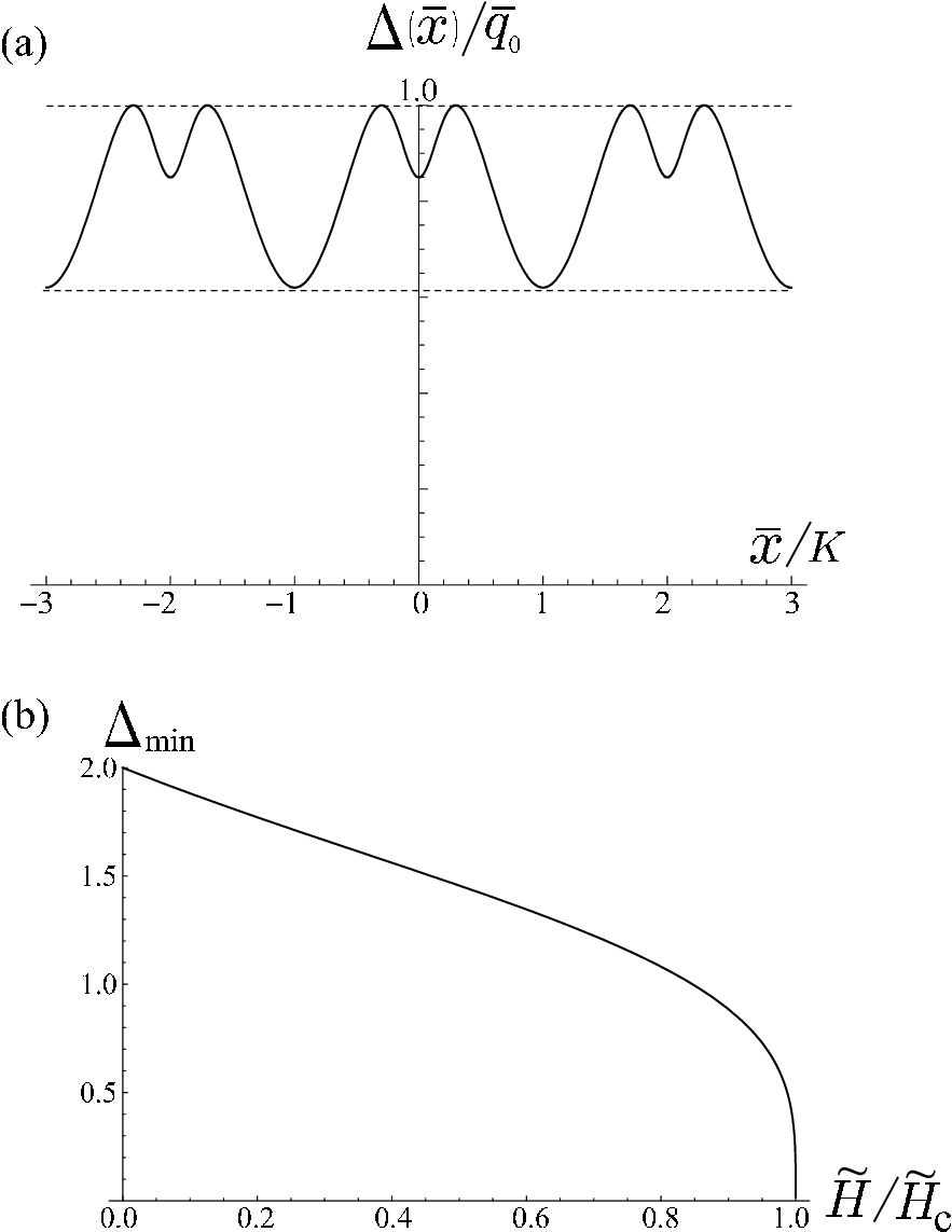
The ”gap function” reads as

where the relation $\partial_{\bar{x}}\varphi_{0}=2\mathrm{dn\,}\left(\bar{x},\kappa\right)$ was used. The minimum and maximum value of the gap are given by

respectively, where $\kappa^{\prime}=\sqrt{1-\kappa^{2}}$ is the complementary modulus. We see that the gap closes at the C-IC transition. In Fig.3 (a), we show the spatial variation of the gap function. The $\kappa$ dependence of the minimum gap is shown in Fig.3 (b). For small $\kappa$, we have $\Delta_{\max}\simeq 2-\kappa^{2}/2-3\kappa^{4}/32$, and $\Delta_{\min}\simeq 2-\kappa^{2}/2-7\kappa^{4}/32$. Therefore, $\Delta_{\max}/\Delta_{\min}\simeq 1$ and it is appropriate to approximate $\Delta(\bar{x})\simeq 2$ for the case of weak field. This approximation amounts to approximating $\mathrm{dn\,}\left(\bar{x},\kappa\right)\simeq 1$.

If were we considered only the tangential $\varphi$-mode, our problem reduces to the case first investigated by Sutherland.[38] Furthermore, the $\varphi$-mode is fully studied in the context of the chiral helimagnet.[37, 39] However, to realize the longitudinal magnetic current, as we will see, it is essential to include into consideration the $\theta$-mode. Even of zero-field, $\kappa=0$, the $\theta$-mode acquires the energy gap $\left(JS^{2}\right)\left(m/\kappa\right){\bar{q}}_{0}=DS^{2}$.[22] The $\theta$-gap directly originates from the Dzyaloshinskii interaction that plays a role of easy plane anisotropy. On the other hand, the $\varphi$-mode is the massless Goldstone mode corresponding to rigid rotation of the whole helix around the helical axis.[40] Even after switching the perpendicular field, the $\theta$-mode ($\varphi$-mode) remains to be massive (massless).

The mode expansion is

where the orthonormal basis $v_{\alpha}(\bar{x})$ and $u_{\alpha}(\bar{x})$ is determined through the eigenvalue equations,

with a mode index $\alpha$. The vibrational part is now given by

In explicit form the eigensystem (12) present the Schrödinger-type equations,

In Eq. (15) we consider the case of weak field corresponding to small $\kappa$ that admit $\mathrm{dn\,}\left(\bar{x},\kappa\right)\simeq 1$. In appendix A, we present the general scheme to treat the periodic potential having the spatial period $2K$ and show that this approximation does not affect qualitative result presented below. Now, both equations (15) and (14) reduce to the Jacobi form of the Lam$\acute{\mathrm{e}}$ equation,[41] and their solutions have been discussed by us previously[22] (see also Appendix B). The analysis shows that both the $\varphi$ and $\vartheta$ mode consist of two bands,[38] i.e.,

where the real parameter $a$ runs over $\ K^{\prime}<a\leq K^{\prime}$. Here, $K^{\prime}$ means the complete elliptic integral of the first kind with the complementary modulus $\kappa^{\prime}=\sqrt{1-\kappa^{2}}$.

By imposing the periodic boundary condition, the quasi-momentum (Floquet index) is introduced for the acoustic

($0\leq|Q_{a}^{(-)}|\leq{\pi}/{2K}$) and the optic

(${\pi}/{2K}\leq|Q_{a}^{(-)}|$) branches, respectively, where $Z$ denotes the Jacobi’s Zeta-function.[41] The representation was given by Izyumov and Laptev,[37] and differs from a conventional representation.[41, 38]

A dispersion relation is given by $\omega$ as a function of Floquet index $Q$. We show the excitation spectra $\omega_{\varphi}$ and $\omega_{\vartheta}$ in Fig. 4. Because $4/\pi<{\bar{q}_{0}}\leq 2,$ the energy gap of the $\vartheta$ mode, $\Delta_{\vartheta}(a=0)=\sqrt{2{\bar{q}}_{0}-2},$ has a range $\sqrt{8/\pi-2}<\Delta\leq\sqrt{2}.$ The gap has a maximum value $\Delta_{\vartheta}=\sqrt{2}$ at zero field ($\kappa=0$) and monotonously decreases as the field increases up to the critical field ($\kappa=1$). The normalized wave function at the bottom of the acoustic band is

In the next section we demonstrate that ${\Lambda}_{{\alpha=0}}(\bar{x})$ exactly corresponds to the zero translational mode.

In the previous section, we determined the phonon modes. Next we consider the translational mode. The translational symmetry holds after the kink formation and gives rise to the Goldstone mode, i.e. zero mode $\partial_{\bar{x}}\varphi_{0}\left(\bar{x}\right)=2\mathrm{dn\,}\left(\bar{x},\kappa\right)$. Although the Gaussian fluctuations around the kink crystal state are assumed to be small, this is not true for the zero mode which describes fluctuations without damping. Then, the center of mass coordinate is elevated to the status of the dynamical variable $X(t)$ and the phonon modes are orthogonal to the zero mode. To describe this situation, we follow the collective coordinate method.[42, 43]

At first, we construct the Lagrangian for the kink crystal system. We make use of the coherent states of spins,

where

with $\mathbf{n}_{i}=(\cos\theta_{i},\sin\theta_{i}\cos\varphi_{i},\sin\theta_{i}\sin\varphi_{i})$ and $\mathbf{n}_{0}=(1,0,0).$ $S_{i}(i=x,y,z)$ are the generators of SU(2) in the spin-$S$ representation and satisfy $\left[S_{\alpha},S_{\beta}\right]=i\epsilon_{\alpha\beta\gamma}S_{\gamma}.$ The highest weight state $\left|S,S\right\rangle$ satisfies $S_{i}^{x}\left|S,S\right\rangle=S\left|S,S\right\rangle$ and $\mathbf{S}^{2}\left|S,S\right\rangle=S(S+1)\left|S,S\right\rangle$. The states $\left|\mathbf{n}_{i}\right\rangle$ form an overcomplete set and give $\left\langle\mathbf{n}_{i}\right|\mathbf{S}\left|\mathbf{n}_{i}\right\rangle=S\mathbf{n}_{i}.$ Using this representation, the Berry phase contribution to the real-time Lagrangian per unit area is written as

where we took the continuum limit in the second line. Now, we construct the Lagrangian,

with the coefficients

and expand $\varphi$ and $\theta$ in the form,

In the expansion of the $\theta$-mode, it is not necessary to exclude $\alpha=0$, since the $\theta$-mode does not contain zero mode. This description amounts to using the curvilinear basis, $\left\{X,\eta_{\alpha},\xi_{\alpha}\right\},$ in functional space and taking the generalized coordinates $q_{1}=\overline{X}$, $q_{2\alpha}=\eta_{\alpha}$, $q_{3\alpha}=\xi_{\alpha}$. Since the zero mode $\partial_{\bar{x}}\varphi_{0}\left(\bar{x}\right)$ is orthogonal to the phonon modes, we have

for $\alpha\neq 0.$ Noting that

and

and plugging these expressions into the Lagrangian (24), we obtain

where higher order terms ${\mathcal{O}}\left(q^{3}\right)$ are dropped. The overlap coefficients are given by

The Lagrangian (28) is singular because it does not contain any term of the form $\dot{q}_{i}\dot{q}_{j}$, and the rank of the Hessian matrix $\left({\partial}^{2}{\mathcal{L}}/{\partial}\dot{q}_{i}{\partial}\dot{q}_{j}\right)$ becomes zero. This means that there is no primary expressible velocities. Therefore we need to construct the Hamiltonian by using the Dirac’s algorithm for the constrained Hamiltonian systems.[44, 45] The details of the treatment have been given in our previous treatment (see, also Appendix C). The final result is

which means that only finite amplitude of the $\vartheta$-mode,

appears when the collective velocity $\dot{X}$ is finite. This is exactly the manifestation of the ODLRO. In other words, the $u(\bar{x})$-field is interpreted as the demagnetization field that drives the inertial motion of the kink. Using Eq.(31), we reach the final form of the physical Hamiltonian,

where the inertial mass of the kink crystal is introduced

The physical Hamiltonian (33) describes the inertial motion of the kink crystal.

The linear momentum per unit area carried by the kink crystal may be presented in the form[22] $P=2\pi\hslash S{\mathcal{Q}}+M\dot{X}$, where the topological charge

is introduced. Apparently, the transverse magnetic field increases a period of the kink crystal lattice and diminishes the topological charge ${\mathcal{Q}}$ and therefore it affects only the background linear momentum (see discussion in Sec. VI). The physical momentum related with a mass transport due to the excitations around the kink crystal state is generated by the steady movement.

The “superfluid magnon current”  transferred by the $\theta$-fluctuations is determined through the definition of the accumulated magnon density[15] $\mathcal{\rho}_{\text{s}}$ in the total magnon density $\mathcal{N}=g\mu_{\text{B}}S\left(1-\cos\theta\right)$ $=\mathcal{\rho}_{\text{0}}+\mathcal{\rho}_{\text{s}}$, where the superfluid part $\mathcal{\rho}_{\text{s}}=-g\mu_{\text{B}}S\cos\theta$ is conjugated with the magnon time-even current carried by the $\theta$-fluctuations

via a continuity equation.[22] The important point is that the only massive $\theta$-mode can carry the longitudinal magnon current as a manifestation of ordering in non-equilibrium state, i.e., dynamical off-diagonal long range order.[46]

The net magnetization (magnetic dipole moment) induced by the movement is

The minus sign means that the net magnetization produces a demagnetization field.

To compute the mass $M$, the spin current $j^{x}$ and the magnetic dipole moment $m$, we consider an array of parallel chains described by the model (1), where a number of chains per unit area is $n_{\text{area}}=1/a_{0}^{2}$. In the case of the molecular-based chiral magnets, the crystal packing is usually loose ($a_{0}\simeq 10^{-9}$[m]) and the exchange interaction is rather weak ($J\simeq 10$[K] $\simeq 10^{-22}$[J]). On the other hand, in the case of the inorganic chiral magnets, the crystal packing is close ($a_{0}\simeq 10^{-10}$[m]) and the exchange interaction is rather strong ($J\simeq 100$[K] $\simeq 10^{-21}$[J]). We take these values as just typical parameter choices. The strength of the Dzyaloshinskii interaction is ambiguous and we simply take $q_{0}=D/J=10^{-2}$.

References

- [1] I. Žutić, J. Fabian, and S. Das. Sarma, Rev. Mod. Phys. 76, 323 (2004) and references therein.
- [2] J. C. Slonczewski, J. Magn. Magn. Mater. 159, L1 (1996).
- [3] L. Berger, Phys. Rev. B54, 9353 (1996).
- [4] M. D. Stiles and A. Zangwill, J. Appl. Phys. 91, 6812 (2002).
- [5] M. D. Stiles and A. Zangwill, Phys. Rev. B66, 014407 (2002).
- [6] G. Tatara and H. Kohno, Phys. Rev. Lett. 92, 086601(2004).
- [7] Y. Aharonov and A. Stern, Phys. Rev. Lett. 69, 3593 (1992).
- [8] Ya. B. Bazaliy, B. A. Jones, and S.-C. Zhang, Phys. Rev. B 57, R3213 (1998).
- [9] E. I. Rashba, Sov. Phys. Solid State 2, 1109 (1960).
- [10] S. Murakami, N. Nagaosa, and S. C. Zhang, Science 301, 1348 (2003).
- [11] J. Sinova, D. Culcer, Q. Niu, N. A. Sinitsyn, T. Jungwirth, and A. H. MacDonald, Phys. Rev. Lett. 92, 126603 (2004).
- [12] P. Bruno and V. K. Dugaev, Phys. Rev. B 72, 241302(R) (2005).
- [13] E. I. Rashba, J. Superconductivity, 18, 137 (2005).
- [14] I.A. Fomin, Physica B169, 153 (1991).
- [15] G. E. Volovik, arXiv:cond-mat/0701180.
- [16] L. D. Landau and E. M. Lifshitz, Fluid Mechanics (Pergamon, Oxford, 1984)
- [17] W. Döring, Zeits. f. Naturforschung 3a, 374 (1948).
- [18] R. Becker, Proceedings of the Grenoble Conference, July (1950).
- [19] C. Kittel, Phys. Rev. 80, 918 (1950).
- [20] I. E. Dzyaloshinskii, J. Phys. Chem. Solids 4, 241 (1958).
- [21] J. Kishine, K. Inoue, and Y. Yoshida: Prog. Theoret. Phys., Supplement 159, 82 (2005).
- [22] I.G. Bostrem, J. Kishine, and A. S. Ovchinnikov, Phys. Rev. B 77, 132405 (2008).
- [23] Izumov Yu. A., Naish V. E. and Ozerov R. P., Neutron Diffraction of Magnetic Materials, Consulting Bureau, New York (1991).
- [24] O. V. Kovalev, Representations of the Crystallographic Space Groups Edition 2 (Gordon and Breach Science Publishers, Switzerland, 1993).
- [25] I. E. Dzyaloshinskii, Sov. Phys. JETP 19, 960 (1964); Sov. Phys. JETP 20, 665 (1965).
- [26] Y. Ishikawa, K. Tajima, P. Bloch, and M. Roth, Solid State Commun. 19, 525 (1976).
- [27] T. Moriya and T. Miyadai, Solid State Commun. 42 (1982), 209.
- [28] B. Roessli, J. Schefer, G. A. Petrakovskii, B. Ouladdiaf, M. Boehm1, U. Staub, A. Vorotinov, and L. Bezmaternikh, Phys. Rev. Lett. 86 (2001), 1885.
- [29] Y. Kousaka, S. Yano, J. Kishine, Y. Yoshida, K. Inoue, K. Kikuchi, and Jun Akimitsu, J. Phys. Soc. Jpn.76, 123709 (2007).
- [30] J. Scalapino, Y. Imry, and P. Pincus, Phys. Rev. B 11, 2042 (1975).
- [31] L. L. Liu, Phys. Rev. Lett. 31, 459 (1973).
- [32] J. Rubinstein, J. Math. Phys. 11, 258 (1970).
- [33] P. Bak and J. von Boehm, Phys. Rev. B 21, 5297 (1980).
- [34] L.N. Bulaevskii and D.I. Khomskii, Zh. Eksp. Teor. Fiz. 74, 1863 (1978) [Sov. Phys. JETP 47, 971 (1978)].
- [35] V.L. Pokrovskii and A.L. Talapov, Zh. Eksp. Teor. Fiz. 75, 1151 (1978) [Sov. Phys. JETP 75, 579 (1978)].
- [36] W.L. McMillan, Phys. Rev. B 14, 1496 (1976); ibid. 16, 4655 (1977).
- [37] Yu. A. Izyumov and V. M. Laptev, JETP 62, 755 (1985).
- [38] B. Sutherland, Phys. Rev. A 8, 2514 (1973).
- [39] D. N. Aristov and A. Luther, Phys. Rev. B 65, 165412 (2002).
- [40] R. J. Elliott and R. V. Lange, Phys. Rev. 152, 235 (1966).
- [41] E. T. Whittaker and G. N. Watson, A Course of Modern Analysis (Cambridge University Press, New York, 1927).
- [42] N. H. Christ and T. D. Lee, Phys. Rev. D 12,1606 (1975).
- [43] R. Rajaraman, Solitons and Instantons; An Introduction to Solitons and Instantons in Quantum Field Theory, North-Holland, Amsterdam and New York, (1982).
- [44] P.A.M. Dirac, Lectures on Quantum Mechanics, (Yeshiva, New York, 1964).
- [45] D.M. Gitman, I.V. Tyutin, Quantization of Fields with Constraints, (Springer, Berlin, 1990).
- [46] J. Xiao, A. Zangwill, and M. D. Stiles, Phys. Rev. B 73, 054428 (2006). Nonequillibrium spin currents in this work are considered for free-electron Stoner model for systems with continously nonuniform magnetization.
- [47] J. Heurich and J. König, and A. H. MacDonald, Phys. Rev. B68, 064406 (2003).
- [48] F. Schütz, P. Kopietz, and M. Kollar, Eur. Phys. J. B 41, 557 (2004).
- [49] P. Chandra, P. Coleman and A. I. Larkin, J. Phys.: Condens. Matter 2, 7933 (1990).
- [50] V. I. Fedorov, A. G. Gukasov, V. Kozlov, S. V. Maleyev, V. P. Plakhty, I. A. Zobkalo, Phys. Lett. A 224, 372 (1997).
- [51] B. Hu and J. Tekić, Phys. Rev. Lett. 87, 035502 (2001).
- [52] S. Chikazumi, Physics of Ferromagnetism, Oxford, New York (1996).
- [53] S. Flgge, Practical Quantum Mechanics, Springer-Verlag, Berlin, 1971.
- [54] L.D. Landau and E.M. Lifshitz, Quantum Mechanics, Pergamon, London, (1958).