跳到论文正文
W Papers独立论文阅读器 arXiv:0806.0961 论文正文 计算阅读时间 · 0%
引用这篇论文根据当前论文元数据生成,正式投稿前建议核对。


License: arXiv.org perpetual non-exclusive license
arXiv:0806.0961v1 [math.AP] 05 Jun 2008

Location and phase segregation of ground and
excited states for 2D Gross–Pitaevskii systemsThanks: The research of the second author was partially supported by the MIUR national research project Variational and Topological Methods in the Study of Nonlinear Phenomena

Marco Caliari Current address: Dipartimento di Informatica, Università di Verona, Cà Vignal 2, Strada Le Grazie 15, I-37134 Verona, Italy. Email address: marco.caliari@univr.it and Marco Squassina Current address: Dipartimento di Informatica, Università di Verona, Cà Vignal 2, Strada Le Grazie 15, I-37134 Verona, Italy. Email address: marco.squassina@univr.it Communicated by Charles Li, received December 4, 2007
and, in revised form, February 20, 2008.
© 2008, International Press
Abstract.

We consider a system of Gross–Pitaevskii equations in ℝ2{\mathbb{R}}^{2} modelling a mixture of two Bose–Einstein condensates with repulsive interaction. We aim to study the qualitative behaviour of ground and excited state solutions. We allow two different harmonic and off-centered trapping potentials and study the spatial patterns of the solutions within the Thomas–Fermi approximation as well as phase segregation phenomena within the large-interaction regime.

Key words and phrases: 
Gross–Pitaevskii equations, Bose–Einstein binary condensates, ground states, location of solutions, phase-segregation of solutions
2000 Mathematics Subject Classification
Primary 35B40, 35Q55; Secondary 81V05, 81V45

1. Introduction

The first successful experimental realization of Bose–Einstein condensates for atomic gases [4], which goes back to 1995, gave rise to various numerical and theoretical investigations on the macroscopic equation ruling these phenomena, that is the Gross–Pitaevskii equation (GPE)

ℏ​i​∂tψ=−ℏ22​m​Δ​ψ+V⁡(x)​ψ+ϑ​|ψ|2​ψ,x∈ℝn,ϑ≥0.\hbar i\partial_{t}\psi=-\frac{\hbar^{2}}{2m}\Delta\psi+V(x)\psi+{\vartheta}|\psi|^{2}\psi,\quad\text{$x\in{\mathbb{R}}^{n}$},\quad{\vartheta}\geq 0.

More recently, in 1997, Bose–Einstein condensation for a mixture of two different interacting atomic species with the same mass was firstly realized at JILA [26] exhibiting a partial overlap between the wave functions. The vector nature of the order parameter gives rise to some intriguing structures and dynamics that are absent in the single component case. This, again, stimulated various succeeding studies of numerical and theoretical nature. For both single or binary condensates we refer the reader to [13, 30] and to the references therein. Recently, some efficient numerical techniques have been developed to compute ground state solutions of GPE [6, 9], which can be used to investigate the vector case. On this basis, in this paper we deal with the rigorous analysis of the spatial configurations for the standing wave solutions (ground and excited states) of the system in ℝ2{\mathbb{R}}^{2}

(1.1) {ℏ​i​∂tψ1=−ℏ22​m1​Δ​ψ1+V1​(x1,x2)​ψ1+ϑ11​ℏ2​|ψ1|2​ψ1+ϑ12​ℏ2​|ψ2|2​ψ1,ℏ​i​∂tψ2=−ℏ22​m2​Δ​ψ2+V2​(x1,x2)​ψ2+ϑ21​ℏ2​|ψ1|2​ψ2+ϑ22​ℏ2​|ψ2|2​ψ2,\begin{cases}\hbar i\partial_{t}\psi_{1}=-\frac{\hbar^{2}}{2m_{1}}\Delta\psi_{1}+V_{1}(x_{1},x_{2})\psi_{1}+{\vartheta}_{11}\hbar^{2}|\psi_{1}|^{2}\psi_{1}+{\vartheta}_{12}\hbar^{2}|\psi_{2}|^{2}\psi_{1},\\ \vskip 6.0pt\cr\hbar i\partial_{t}\psi_{2}=-\frac{\hbar^{2}}{2m_{2}}\Delta\psi_{2}+V_{2}(x_{1},x_{2})\psi_{2}+{\vartheta}_{21}\hbar^{2}|\psi_{1}|^{2}\psi_{2}+{\vartheta}_{22}\hbar^{2}|\psi_{2}|^{2}\psi_{2},\end{cases}

for the unknown ψi:ℝ2→ℂ\psi_{i}:{\mathbb{R}}^{2}\to{\mathbb{C}}, i=1,2i=1,2, where ℏ\hbar denotes the (reduced) Planck constant and the coefficients ϑi​j≥0{\vartheta}_{ij}\geq 0 (defocusing case), with ϑ12=ϑ21{\vartheta}_{12}={\vartheta}_{21}, are given by the formula [15]

ϑi​j=2πσi​jmi+mjmi​mj,σi​j=σj​i,i,j=1,2,{\vartheta}_{ij}=2\pi\sigma_{ij}\frac{m_{i}+m_{j}}{m_{i}m_{j}},\quad\sigma_{ij}=\sigma_{ji},\quad i,j=1,2,

being σi​j\sigma_{ij} related to the scattering lengths and mim_{i} the atomic masses of the two species composing the mixture. Considering the 2D case is not restrictive as there are various situations where the full 3D system can be reduced to a 2D system with suitably modified coefficients (see e.g. Section 2.2 of [5]). The coefficients ϑi​i{\vartheta}_{ii} and ϑ12{\vartheta}_{12} play the role of repulsive intra-species and inter-species parameters respectively. As we will see, when ϑ12{\vartheta}_{12} is sufficiently large, then some interesting overlap and spatial segregation phenomena between the wave densities occur. Concerning the potentials, we let Vi​(x1,x2)=mi2​(ωi​12​(x1−xi​1)2+ωi​22​(x2−xi​2)2)V_{i}(x_{1},x_{2})=\frac{m_{i}}{2}(\omega_{i1}^{2}(x_{1}-x_{i1})^{2}+\omega_{i2}^{2}(x_{2}-x_{i2})^{2}) for (x1,x2)(x_{1},x_{2}) in ℝ2{\mathbb{R}}^{2}, where ωi​j>0\omega_{ij}>0, i,j=1,2i,j=1,2. A typical situation is when the ViV_{i}s have the same center, without loss of generality, the origin. On the other hand, there are some physical situations reported in literature, which lead to consider off-centered potentials. See, for instance, [32], where the vertical direction in the potential is not aligned with the symmetry axis of the trap. Similar equations have also arisen as governing equations for electromagnetic pulse propagation in “left-handed” materials with Kerr-type nonlinearity [19], in the modified Hubbard model in the long-wavelength approximation [23, 22], in quadratic nonlinear materials with suitable phase matching [18] and in nonlinear optics, for instance in the propagation of pulses in a nonlinear optical fiber of bi-modal type due to the presence of some birefringence effects generating two pulses with different polarization directions [24]. For a wide discussion on nonlinear Schrödinger systems we refer the interested reader to [1, 2, 3] and to the references therein.

Let ℋ{\mathcal{H}} be the Hilbert subspace of H1​(ℝ2,ℂ)×H1​(ℝ2,ℂ)H^{1}({\mathbb{R}}^{2},{\mathbb{C}})\times H^{1}({\mathbb{R}}^{2},{\mathbb{C}}) defined by

ℋ={(ψ1,ψ2)∈H1(ℝ2,ℂ)×H1(ℝ2,ℂ):∫ℝ2Vi(x1,x2)|ψi|2<∞,i=1,2},{\mathcal{H}}=\left\{(\psi_{1},\psi_{2})\in H^{1}({\mathbb{R}}^{2},{\mathbb{C}})\times H^{1}({\mathbb{R}}^{2},{\mathbb{C}}):\,\,\,\int_{{\mathbb{R}}^{2}}V_{i}(x_{1},x_{2})|\psi_{i}|^{2}<\infty,\,\,\,i=1,2\right\},

which is the natural framework for bound state solutions, endowed with the norm

‖(ψ1,ψ2)‖ℋ2=∑i=12ℏ22​mi​∫ℝ2|∇ψi|2+∫ℝ2Vi​(x1,x2)​|ψi|2,\|(\psi_{1},\psi_{2})\|_{{\mathcal{H}}}^{2}=\sum_{i=1}^{2}\frac{\hbar^{2}}{2m_{i}}\int_{{\mathbb{R}}^{2}}|\nabla\psi_{i}|^{2}+\int_{{\mathbb{R}}^{2}}V_{i}(x_{1},x_{2})|\psi_{i}|^{2},

and consider the total energy functional E:ℋ→ℝE:{\mathcal{H}}\to{\mathbb{R}} associated with (1.1)

(1.2) E⁡(ψ1​(⋅,t),ψ2​(⋅,t))=∑i=12Ei​(ψi​(⋅,t))+ϑ12​ℏ2​∫ℝ2|ψ1​(⋅,t)|2​|ψ2​(⋅,t)|2,E(\psi_{1}(\cdot,t),\psi_{2}(\cdot,t))=\sum_{i=1}^{2}E_{i}(\psi_{i}(\cdot,t))+{\vartheta}_{12}\hbar^{2}\int_{{\mathbb{R}}^{2}}|\psi_{1}(\cdot,t)|^{2}|\psi_{2}(\cdot,t)|^{2},

where, for i=1,2i=1,2, we set

Ei​(ψi​(⋅,t))=ℏ22​mi​∫ℝ2|∇ψi​(⋅,t)|2+∫ℝ2Vi​(x1,x2)​|ψi​(⋅,t)|2+ϑi​i​ℏ22​∫ℝ2|ψi​(⋅,t)|4.E_{i}(\psi_{i}(\cdot,t))=\frac{\hbar^{2}}{2m_{i}}\int_{{\mathbb{R}}^{2}}|\nabla\psi_{i}(\cdot,t)|^{2}+\int_{{\mathbb{R}}^{2}}V_{i}(x_{1},x_{2})|\psi_{i}(\cdot,t)|^{2}+\frac{{\vartheta}_{ii}\hbar^{2}}{2}\int_{{\mathbb{R}}^{2}}|\psi_{i}(\cdot,t)|^{4}.

By multiplying the first equation of system (1.1) by ∂tψ¯1\partial_{t}\bar{\psi}_{1} and the second by ∂tψ¯2\partial_{t}\bar{\psi}_{2}, taking the real parts, integrating and adding the resulting identities, it is readily seen that EE is constant on the solutions, namely E⁡(ψ1​(⋅,t),ψ2​(⋅,t))=E⁡(ψ1​(⋅,0),ψ2​(⋅,0))E(\psi_{1}(\cdot,t),\psi_{2}(\cdot,t))=E(\psi_{1}(\cdot,0),\psi_{2}(\cdot,0)) for any t≥0t\geq 0. Also, as for the case of the single equation, by multiplying the first equation of (1.1) by ψ¯1\bar{\psi}_{1} and the second by ψ¯2\bar{\psi}_{2}, taking the imaginary parts, integrating and adding the resulting identities, it turns out that the total number of particles NiN_{i} of the ii-th species is time independent (preservation of the particle number), namely

(1.3) ∫ℝ2|ψi(⋅,t)|2=Ni,t≥0,i=1,2.\int_{{\mathbb{R}}^{2}}|\psi_{i}(\cdot,t)|^{2}=N_{i},\qquad t\geq 0,\,\,i=1,2.

The ground state (or least energy) solution of (1.1) is a solution with ansatz

(1.4) ψi(x1,x2,t)=e−i​μi​tℏϕi(x1,x2),(x1,x2)∈ℝ2,t≥0,i=1,2,\psi_{i}(x_{1},x_{2},t)=e^{-{\rm i}\frac{\mu_{i}t}{\hbar}}\phi_{i}(x_{1},x_{2}),\qquad(x_{1},x_{2})\in{\mathbb{R}}^{2},\,\,t\geq 0,\,\,\,i=1,2,

where the pair (ϕ1,ϕ2)(\phi_{1},\phi_{2}) is real valued and minimizes functional (1.2) constrained to conditions (1.3) (with ϕi\phi_{i} in place of ψi\psi_{i}). As a consequence, the ϕi\phi_{i}s solve the nonlinear eigenvalue problem in ℝ2{\mathbb{R}}^{2}

(1.5) {−ℏ22​m1​Δ​ϕ1+V1​(x1,x2)​ϕ1+ϑ11​ℏ2​|ϕ1|2​ϕ1+ϑ12​ℏ2​|ϕ2|2​ϕ1=μ1​ϕ1,−ℏ22​m2​Δ​ϕ2+V2​(x1,x2)​ϕ2+ϑ21​ℏ2​|ϕ1|2​ϕ2+ϑ22​ℏ2​|ϕ2|2​ϕ2=μ2​ϕ2,∫ℝ2ϕ12=N1,∫ℝ2ϕ22=N2.\begin{cases}-\frac{\hbar^{2}}{2m_{1}}\Delta\phi_{1}+V_{1}(x_{1},x_{2})\phi_{1}+{\vartheta}_{11}\hbar^{2}|\phi_{1}|^{2}\phi_{1}+{\vartheta}_{12}\hbar^{2}|\phi_{2}|^{2}\phi_{1}=\mu_{1}\phi_{1},\\ \vskip 6.0pt\cr-\frac{\hbar^{2}}{2m_{2}}\Delta\phi_{2}+V_{2}(x_{1},x_{2})\phi_{2}+{\vartheta}_{21}\hbar^{2}|\phi_{1}|^{2}\phi_{2}+{\vartheta}_{22}\hbar^{2}|\phi_{2}|^{2}\phi_{2}=\mu_{2}\phi_{2},\\ \vskip 6.0pt\cr\,\,\,\displaystyle\int_{{\mathbb{R}}^{2}}\phi_{1}^{2}=N_{1},\,\,\,\int_{{\mathbb{R}}^{2}}\phi_{2}^{2}=N_{2}.\end{cases}

Testing the first equation of (1.5) by ψ¯1\bar{\psi}_{1} and the second by ψ¯2\bar{\psi}_{2}, we have a formula for the eigenvalues μi\mu_{i} (also known as chemical potentials) versus the eigenvectors ϕi\phi_{i}

(1.6) Niμi=Ei(ϕi)+ϑi​i2ℏ2∫ℝ2|ϕi|4+ϑ12ℏ2∫ℝ2|ϕ1|2|ϕ2|2,i=1,2.N_{i}\mu_{i}=E_{i}(\phi_{i})+\frac{{\vartheta}_{ii}}{2}\hbar^{2}\int_{{\mathbb{R}}^{2}}|\phi_{i}|^{4}+{\vartheta}_{12}\hbar^{2}\int_{{\mathbb{R}}^{2}}|\phi_{1}|^{2}|\phi_{2}|^{2},\qquad i=1,2.

The existence of ground state solutions to (1.1) in ℋ{\mathcal{H}} is reduced to the existence of minima for the energy functional (1.2) constrained to

(1.7) 𝒮={(ϕ1,ϕ2)∈ℋ:∥ϕi∥L22=Ni,i=1,2}.{\mathcal{S}}=\{(\phi_{1},\phi_{2})\in{\mathcal{H}}:\,\|\phi_{i}\|_{L^{2}}^{2}=N_{i},\,\,\text{$i=1,2$}\}.

As the ϑi​j{\vartheta}_{ij} are positive,

ϑ112​|ϕ1|4+ϑ12​|ϕ1|2​|ϕ2|2+ϑ222​|ϕ2|4≥0,\frac{{\vartheta}_{11}}{2}|\phi_{1}|^{4}+{\vartheta}_{12}|\phi_{1}|^{2}|\phi_{2}|^{2}+\frac{{\vartheta}_{22}}{2}|\phi_{2}|^{4}\geq 0,

so that the energy functional EE is coercive, bounded from below and weakly lower semi-continuous over 𝒮{\mathcal{S}}. Hence, the existence of a ground state solution is immediately guaranteed. Usually, with reference to the solutions of the form (1.4) (standing waves), there are two possible (physically different) approaches depending on whether one considers the chemical potentials μi\mu_{i} as fixed (hence searching for solutions to the first two equations in (1.5) but with possibly different L2L^{2} norms) or the total masses ∫ℝ2|ϕi|2\int_{{\mathbb{R}}^{2}}|\phi_{i}|^{2} as fixed (thus solving the nonlinear eigenvalue problem (1.5), which is the case we deal with). Any other solution (ϕ1,ϕ2)(\phi_{1},\phi_{2}) of system (1.5) of the form (1.4) not having minimal energy for EE will be called excited state (or higher energy solution).

The main goal of this paper is to prove some geometrical properties (clearly confirmed by some numerical simulations) for ground and excited state of (1.5), particularly under the influence of strong interaction effects (namely ϑ12→∞{\vartheta}_{12}\to\infty). See e.g. Propositions 3.1 and 3.2.

In Section 2 we derive the location of ground state solutions via the Thomas–Fermi approximation and classify the relative configuration of ϕi\phi_{i} with respect to ϕj\phi_{j}. In Section 3 we study the phase separation process (spatial segregation) in the large competition regime by means of suitable limiting energy levels which provide κ\kappa-independent upper bounds for the energy of solutions. In Section 4, for the sake of completeness, we briefly describe the functional framework of the numerical scheme used to compute the solutions.

In the following the Hilbert space L2​(ℝ2,ℂ)L^{2}({\mathbb{R}}^{2},{\mathbb{C}}) is endowed with the standard scalar product (f,g)2=∫ℝ2f​g¯(f,g)_{2}=\int_{{\mathbb{R}}^{2}}f\bar{g}, f,g∈L2​(ℝ2)f,g\in L^{2}({\mathbb{R}}^{2}) and the induced norm is denoted by ∥⋅∥L2\|\cdot\|_{L^{2}}.

2. Location and Thomas–Fermi approximation

If the distance between the centers of the trapping potentials ViV_{i} is sufficiently small compared with the radii of the supports of the ground state solutions ϕi\phi_{i}, then the condensates share a region where they coexist (with a partial or full overlap, that is one condensate is partially or entirely included in the other). In the opposite case the supports of the wave functions are disjoint. Hence, we can encounter three different patterns for the spatial wave functions ϕi\phi_{i}, which we are going to discuss, namely: no overlap, partial overlap and full overlap. It should be noted that support just means here the planar region where the mass of the ground state solution is mainly concentrated, being (exponentially) vanishing on the outside. In the Thomas–Fermi regime, an approximation of the ground state solutions of system (1.5), which is very good for sufficiently large values of the coupling constants, can be obtained by simply dropping the diffusion terms −Δ​ϕi-\Delta\phi_{i}, namely the kinetic contributions, thus assuming the wave functions to be slowly varying (cf. [16, 35, 20, 21]). In turn, (1.5) reduces to the algebraic system (here we let ℏ=1\hbar=1)

(2.1) {2​ϑ11​|ϕ1|2+2​ϑ12​|ϕ2|2=2​μ1−(x1−x11)2−(x2−x12)2,2​ϑ21​|ϕ1|2+2​ϑ22​|ϕ2|2=2​μ2−(x1−x21)2−(x2−x22)2,\begin{cases}2{\vartheta}_{11}|\phi_{1}|^{2}+2{\vartheta}_{12}|\phi_{2}|^{2}=2\mu_{1}-(x_{1}-x_{11})^{2}-(x_{2}-x_{12})^{2},\\ \vskip 5.0pt\cr 2{\vartheta}_{21}|\phi_{1}|^{2}+2{\vartheta}_{22}|\phi_{2}|^{2}=2\mu_{2}-(x_{1}-x_{21})^{2}-(x_{2}-x_{22})^{2},\end{cases}

where the μi\mu_{i}s should be computed through the normalization conditions (1.3) (if, for instance, ϑ12=0{\vartheta}_{12}=0, it holds μi∝ϑi​i\mu_{i}\propto\sqrt{{\vartheta}_{ii}} for i=1,2i=1,2). In general, as the left-hand sides are positive, this system is satisfied only on a (possibly empty) subset 𝒪⊂ℝ2{\mathcal{O}}\subset{\mathbb{R}}^{2} (𝒪=𝒪1∩𝒪2{\mathcal{O}}={\mathcal{O}}_{1}\cap{\mathcal{O}}_{2} in the notations introduced below), namely the overlap region. It is natural to introduce the circumferences defined by (x1−xi​1)2+(x2−xi​2)2=ri2(x_{1}-x_{i1})^{2}+(x_{2}-x_{i2})^{2}=r_{i}^{2}, with ri​(μi)=2​μir_{i}(\mu_{i})=\sqrt{2\mu_{i}}, i=1,2i=1,2. The intersection of the corresponding disks 𝒟i{\mathcal{D}}_{i} gives the region where system (2.1) makes sense. Outside the region 𝒪{\mathcal{O}}, the wave functions take the usual form of the solutions of the GPE (ϑ12=0{\vartheta}_{12}=0) in the Thomas–Fermi regime (see the expressions below of ϕi\phi_{i} on 𝒟i∖𝒪{\mathcal{D}}_{i}\setminus{\mathcal{O}}). More precisely, we have the following non-smooth approximations of the ground state (see also the work by Riboli and Modugno [32])

ϕ1={ϑ22​(2​μ1−(x1−x11)2−(x2−x12)2)−ϑ12​(2​μ2−(x1−x21)2−(x2−x22)2)2​(ϑ11​ϑ22−ϑ122),in 𝒪,2​μ1−(x1−x11)2−(x2−x12)22​ϑ11,in 𝒟1∖𝒪,0,in ℝ2∖𝒟1,\phi_{1}=\begin{cases}\sqrt{\frac{{\vartheta}_{22}(2\mu_{1}-(x_{1}-x_{11})^{2}-(x_{2}-x_{12})^{2})-{\vartheta}_{12}(2\mu_{2}-(x_{1}-x_{21})^{2}-(x_{2}-x_{22})^{2})}{2({\vartheta}_{11}{\vartheta}_{22}-{\vartheta}_{12}^{2})}},&\text{in ${\mathcal{O}}$},\\ \vskip 3.0pt\cr\sqrt{\frac{2\mu_{1}-(x_{1}-x_{11})^{2}-(x_{2}-x_{12})^{2}}{2{\vartheta}_{11}}},&\text{in ${\mathcal{D}}_{1}\setminus{\mathcal{O}}$},\\ \vskip 7.0pt\cr 0,&\text{in ${\mathbb{R}}^{2}\setminus{\mathcal{D}}_{1}$},\end{cases}
ϕ2={ϑ11​(2​μ2−(x1−x21)2−(x2−x22)2)−ϑ12​(2​μ1−(x1−x11)2−(x2−x12)2)2​(ϑ11​ϑ22−ϑ122),in 𝒪,2​μ2−(x1−x21)2−(x2−x22)22​ϑ22,in 𝒟2∖𝒪,0,in ℝ2∖𝒟2,\phi_{2}=\begin{cases}\sqrt{\frac{{\vartheta}_{11}(2\mu_{2}-(x_{1}-x_{21})^{2}-(x_{2}-x_{22})^{2})-{\vartheta}_{12}(2\mu_{1}-(x_{1}-x_{11})^{2}-(x_{2}-x_{12})^{2})}{2({\vartheta}_{11}{\vartheta}_{22}-{\vartheta}_{12}^{2})}},&\text{in ${\mathcal{O}}$},\\ \vskip 3.0pt\cr\sqrt{\frac{2\mu_{2}-(x_{1}-x_{21})^{2}-(x_{2}-x_{22})^{2}}{2{\vartheta}_{22}}},&\text{in ${\mathcal{D}}_{2}\setminus{\mathcal{O}}$},\\ \vskip 7.0pt\cr 0,&\text{in ${\mathbb{R}}^{2}\setminus{\mathcal{D}}_{2}$},\end{cases}

that is, equivalently,

(2.2) ϕi={αi​(Ri2−(x1−yi​1)2−(x2−yi​2)2),in 𝒪,ri2−(x1−xi​1)2−(x2−xi​2)22​ϑi​i,in 𝒟i∖𝒪,0,in ℝ2∖𝒟i,\phi_{i}=\begin{cases}\sqrt{\alpha_{i}(R_{i}^{2}-(x_{1}-y_{i1})^{2}-(x_{2}-y_{i2})^{2})},&\text{in ${\mathcal{O}}$},\\ \vskip 3.0pt\cr\sqrt{\frac{r_{i}^{2}-(x_{1}-x_{i1})^{2}-(x_{2}-x_{i2})^{2}}{2{\vartheta}_{ii}}},&\text{in ${\mathcal{D}}_{i}\setminus{\mathcal{O}}$},\\ \vskip 6.0pt\cr 0,&\text{in ${\mathbb{R}}^{2}\setminus{\mathcal{D}}_{i}$},\end{cases}

where, according to the notations introduced below, 𝒪=𝒪1∩𝒪2{\mathcal{O}}={\mathcal{O}}_{1}\cap{\mathcal{O}}_{2}, 𝒟=𝒟1∩𝒟2{\mathcal{D}}={\mathcal{D}}_{1}\cap{\mathcal{D}}_{2},

𝒪i\displaystyle{\mathcal{O}}_{i} ={(x1,x2)∈𝒟:(x1−yi​1)2+(x2−yi​2)2≤(≥)​Ri2},\displaystyle=\big\{(x_{1},x_{2})\in{\mathcal{D}}:\,\,(x_{1}-y_{i1})^{2}+(x_{2}-y_{i2})^{2}\leq(\geq)R_{i}^{2}\big\},
𝒟i\displaystyle{\mathcal{D}}_{i} ={(x1,x2)∈ℝ2:(x1−xi​1)2+(x2−xi​2)2≤ri2},\displaystyle=\big\{(x_{1},x_{2})\in{\mathbb{R}}^{2}:\,\,(x_{1}-x_{i1})^{2}+(x_{2}-x_{i2})^{2}\leq r_{i}^{2}\big\},

with ≤\leq (resp. ≥\geq) in the definition of 𝒪i{\mathcal{O}}_{i} for αi>0\alpha_{i}>0 (resp. αi<0\alpha_{i}<0), if we set

y11\displaystyle y_{11} =ω22​x11−ω12​x21ω22−ω12=x11+ω12α1​Δ1​x,y12=ω22​x12−ω12​x22ω22−ω12=x12+ω12α1​Δ2​x,\displaystyle=\frac{\omega_{22}x_{11}-\omega_{12}x_{21}}{\omega_{22}-\omega_{12}}=x_{11}+\frac{\omega_{12}}{\alpha_{1}}\Delta_{1}x,\quad y_{12}=\frac{\omega_{22}x_{12}-\omega_{12}x_{22}}{\omega_{22}-\omega_{12}}=x_{12}+\frac{\omega_{12}}{\alpha_{1}}\Delta_{2}x,
y21\displaystyle y_{21} =ω11​x21−ω12​x11ω11−ω12=x21−ω12α2​Δ1​x,y22=ω11​x22−ω12​x12ω11−ω12=x22−ω12α2​Δ2​x,\displaystyle=\frac{\omega_{11}x_{21}-\omega_{12}x_{11}}{\omega_{11}-\omega_{12}}=x_{21}-\frac{\omega_{12}}{\alpha_{2}}\Delta_{1}x,\quad y_{22}=\frac{\omega_{11}x_{22}-\omega_{12}x_{12}}{\omega_{11}-\omega_{12}}=x_{22}-\frac{\omega_{12}}{\alpha_{2}}\Delta_{2}x,

where Δj​x=x1​j−x2​j\Delta_{j}x=x_{1j}-x_{2j}, namely, for i,j=1,2i,j=1,2 with i≠ji\neq j,

yi​j=xi​j−(−1)i​ω12αi​Δj​x,y_{ij}=x_{ij}-(-1)^{i}\frac{\omega_{12}}{\alpha_{i}}\Delta_{j}x,

with ωi​j=ϑi​j2​d​e​t​Θ\omega_{ij}=\frac{{\vartheta}_{ij}}{2{\rm det}\,\Theta}, i,j=1,2i,j=1,2, α1=ω22−ω12\alpha_{1}=\omega_{22}-\omega_{12}, α2=ω11−ω12\alpha_{2}=\omega_{11}-\omega_{12}, and

R12\displaystyle R_{1}^{2} =2​ω22​μ1−2​ω12​μ2+ω12​x212+ω12​x222−ω22​x112−ω22​x122ω22−ω12+y112+y122\displaystyle=\frac{2\omega_{22}\mu_{1}-2\omega_{12}\mu_{2}+\omega_{12}x_{21}^{2}+\omega_{12}x_{22}^{2}-\omega_{22}x_{11}^{2}-\omega_{22}x_{12}^{2}}{\omega_{22}-\omega_{12}}+y_{11}^{2}+y_{12}^{2}
R22\displaystyle R_{2}^{2} =2​ω11​μ2−2​ω12​μ1+ω12​x112+ω12​x122−ω11​x212−ω11​x222ω11−ω12+y222+y212.\displaystyle=\frac{2\omega_{11}\mu_{2}-2\omega_{12}\mu_{1}+\omega_{12}x_{11}^{2}+\omega_{12}x_{12}^{2}-\omega_{11}x_{21}^{2}-\omega_{11}x_{22}^{2}}{\omega_{11}-\omega_{12}}+y_{22}^{2}+y_{21}^{2}.

Setting 𝐱𝐢=(xi​1,xi​2){\bf x_{i}}=(x_{i1},x_{i2}) and 𝐲𝐢=(yi​1,yi​2){\bf y_{i}}=(y_{i1},y_{i2}) for i=1,2i=1,2, this reads as

Ri=ri2+2​ω12αi​(μi−μj)+ω12αi​(|𝐱𝐣|2−|𝐲𝐢|2)−ωj​jαi​(|𝐱𝐢|2−|𝐲𝐢|2).R_{i}=\sqrt{r_{i}^{2}+\frac{2\omega_{12}}{\alpha_{i}}(\mu_{i}-\mu_{j})+\frac{\omega_{12}}{\alpha_{i}}(|{\bf x_{j}}|^{2}-|{\bf y_{i}}|^{2})-\frac{\omega_{jj}}{\alpha_{i}}(|{\bf x_{i}}|^{2}-|{\bf y_{i}}|^{2})}.

Hence, we have four circumferences that rule the geometry of the ground states

Σir:(x1−xi​1)2+(x2−xi​2)2=ri2,ΣiR:(x1−yi​1)2+(x2−yi​2)2=Ri2.\Sigma_{i}^{r}:\,(x_{1}-x_{i1})^{2}+(x_{2}-x_{i2})^{2}=r_{i}^{2},\qquad\Sigma_{i}^{R}:\,(x_{1}-y_{i1})^{2}+(x_{2}-y_{i2})^{2}=R_{i}^{2}.

If ϑ12=0{\vartheta}_{12}=0 (namely no interaction), we deduce that 𝐱𝐢=𝐲𝐢{\bf x_{i}}={\bf y_{i}}, Ri=riR_{i}=r_{i}, and 𝒪i=𝒟i{\mathcal{O}}_{i}={\mathcal{D}}_{i} (ϑ12=0{\vartheta}_{12}=0 implies αi>0\alpha_{i}>0), so that the ground state solutions turn into the usual Thomas–Fermi representation for the single GPE

ϕi={ri2−(x1−xi​1)2−(x2−xi​2)22​ϑi​i,in 𝒟i,0,in ℝ2∖𝒟i.\phi_{i}=\begin{cases}\sqrt{\frac{r_{i}^{2}-(x_{1}-x_{i1})^{2}-(x_{2}-x_{i2})^{2}}{2{\vartheta}_{ii}}},&\text{in ${\mathcal{D}}_{i}$},\\ \vskip 4.0pt\cr 0,&\text{in ${\mathbb{R}}^{2}\setminus{\mathcal{D}}_{i}$}.\end{cases}

If ϑ12≈0{\vartheta}_{12}\approx 0, then ω11≈12​ϑ22\omega_{11}\approx\frac{1}{2{\vartheta}_{22}}, ω22≈12​ϑ11\omega_{22}\approx\frac{1}{2{\vartheta}_{11}}, ω12≈0\omega_{12}\approx 0, αi≈12​ϑi​i\alpha_{i}\approx\frac{1}{2{\vartheta}_{ii}} and yi​j≈xi​jy_{ij}\approx x_{ij}, Ri≈riR_{i}\approx r_{i} for i,j=1,2i,j=1,2, so that ΣiR≈Σir\Sigma_{i}^{R}\approx\Sigma_{i}^{r} for i=1,2i=1,2. If 𝐱𝟏=𝐱𝟐{\bf x_{1}}={\bf x_{2}}, the ΣiR\Sigma_{i}^{R}s have centers 𝐲𝐢=𝐱𝐢{\bf y_{i}}={\bf x_{i}} but different radii Ri2=ri2+2​ω12αi​(μi−μj)R_{i}^{2}=r_{i}^{2}+\frac{2\omega_{12}}{\alpha_{i}}(\mu_{i}-\mu_{j}), for any i≠ji\neq j.

2.1. Nonoverlap case

In the case occurring when the constant ϑ12{\vartheta}_{12} is zero (absence of interaction in the mixture), the system uncouples into a pair of GPEs (for the single GPE various accurate and efficient numerical techniques have been recently compared in [9]). Numerical experiments show that the ground state solution ϕi\phi_{i} always locates its mass around the minimum point 𝐱𝐢=(xi​1,xi​2){\bf x_{i}}=(x_{i1},x_{i2}) of ViV_{i}, for i=1,2i=1,2. It looks apparent that boosting up the parameter ϑi​i{\vartheta}_{ii} in front of the cubic nonlinearity in the equation of ϕi\phi_{i} has the effect of squeezing down the profile of ϕi\phi_{i} making it flatter and larger. Going back to the case ϑ12≠0{\vartheta}_{12}\neq 0, we say that we have no overlap between ϕ1\phi_{1} and ϕ2\phi_{2}, if the centers 𝐱𝟏{\bf x_{1}} and 𝐱𝟐{\bf x_{2}} of Σir\Sigma_{i}^{r} satisfy the geometric condition

(2.3) (Δ1​x)2+(Δ2​x)2>|2​μ1+2​μ2|2,(\Delta_{1}x)^{2}+(\Delta_{2}x)^{2}>|\sqrt{2\mu_{1}}+\sqrt{2\mu_{2}}|^{2},

namely if 𝐱𝟏{\bf x_{1}} is sufficiently far from 𝐱𝟐{\bf x_{2}} with respect to the amplitudes rir_{i} of the supports of ϕi\phi_{i}. In this situation the ground state solutions look like those of the decoupled case. In fact, the coupling terms Ci​j=ϑ12​|ϕj|2​ϕiC_{ij}={\vartheta}_{12}|\phi_{j}|^{2}\phi_{i} with i≠ji\neq j are almost everywhere zero as the supports are disjoint, due to (2.3). Hence the system is actually a small deformation of a pair of uncoupled GPEs. See Figure 1.

Refer to caption
Refer to caption
Figure 1. Supports of ϕ1\phi_{1} and ϕ2\phi_{2} (starred) and disks (unstarred) related to the Thomas–Fermi approximation for ϕ1\phi_{1} and ϕ2\phi_{2}. We have taken N1=N2=m1=m2=1N_{1}=N_{2}=m_{1}=m_{2}=1, ϑ11=400{\vartheta}_{11}=400, ϑ22=200{\vartheta}_{22}=200, ϑ12=100{\vartheta}_{12}=100, x11=4.5x_{11}=4.5, x21=−4.5x_{21}=-4.5 (left figure, tangential supports); and x11=6x_{11}=6, x21=−6x_{21}=-6 (right figure, disjoint supports), with xi​j=0x_{ij}=0 for any other i,ji,j.

2.2. Partial overlap case

We have partial overlap between ϕ1\phi_{1} and ϕ2\phi_{2}, if

|2​μ1−2​μ2|2<(Δ1​x)2+(Δ2​x)2<|2​μ1+2​μ2|2,|\sqrt{2\mu_{1}}-\sqrt{2\mu_{2}}|^{2}<(\Delta_{1}x)^{2}+(\Delta_{2}x)^{2}<|\sqrt{2\mu_{1}}+\sqrt{2\mu_{2}}|^{2},

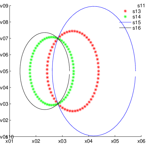
namely the disks of boundaries Σ1r\Sigma_{1}^{r} and Σ2r\Sigma_{2}^{r} overlap without being one completely embedded in the other. We see in the contour plot of Figure 5 the partial overlap in the case ϑ11≫ϑ22{\vartheta}_{11}\gg{\vartheta}_{22}. Apparently, boosting ϑ11{\vartheta}_{11} with respect to ϑ22{\vartheta}_{22} makes the overlap region more localized. Keeping in mind the behaviour of the uncoupled case, in order to give this fact a very simple empirical explanation, it suffices to argue on the coupling terms Ci​jC_{ij}. In the region (depending upon the relative magnitude of the ϑi​i{\vartheta}_{ii}s) where both ϕi\phi_{i} are nonzero the contribution of Ci​jC_{ij} pushes down the profile around the origin (the center of trapping for ϕ2\phi_{2}), provided that ϑ12{\vartheta}_{12} is significantly large. The support of ϕ1\phi_{1} still remains contractible, but the radial symmetry property of ϕ1\phi_{1} is broken (due to strong interaction). See e.g. the situations reported in Figures 2 and 5. As Figure 4 shows, while the Thomas–Fermi approximation disks ΣiR\Sigma_{i}^{R} are overlapped to the support disks Σir\Sigma_{i}^{r} when the coupling constant ϑ12{\vartheta}_{12} is much smaller than the ϑi​i{\vartheta}_{ii}s, in the case where ϑ12≫ϑi​i{\vartheta}_{12}\gg{\vartheta}_{ii}, i.e. in the large interaction regime, the four circumferences intersect in two points and Σir\Sigma_{i}^{r} and ΣiR\Sigma_{i}^{R} may have quite different sizes.

Refer to caption
Figure 2. Supports of ϕ1\phi_{1} and ϕ2\phi_{2} (starred) and disks (unstarred) related to the Thomas–Fermi approximation for ϕ1\phi_{1} and ϕ2\phi_{2} (partial overlap case). We have N1=N2=m1=m2=1N_{1}=N_{2}=m_{1}=m_{2}=1, ϑ11=400{\vartheta}_{11}=400, ϑ22=200{\vartheta}_{22}=200, ϑ12=100{\vartheta}_{12}=100, x11=2x_{11}=2, x21=−2x_{21}=-2 and xi​j=0x_{ij}=0 for other i,ji,j.

2.3. Full overlap case

We have full overlap between ϕ1\phi_{1} and ϕ2\phi_{2}, if

(Δ1​x)2+(Δ2​x)2<|2​μ1−2​μ2|2,(\Delta_{1}x)^{2}+(\Delta_{2}x)^{2}<|\sqrt{2\mu_{1}}-\sqrt{2\mu_{2}}|^{2},

so that the disks of boundaries Σ1r\Sigma_{1}^{r} and Σ2r\Sigma_{2}^{r} are included one in the other, see Figure 3. In a highly interacting regime, this configuration leads to a non-contractible support for one of the two wave functions, which looses the symmetry properties of the trap. If the potentials are both centered at the origin, ϑ11≫ϑ22{\vartheta}_{11}\gg{\vartheta}_{22}, and the coupling ϑ12{\vartheta}_{12} is sufficiently large, as ϕ2\phi_{2} spikes around the origin, ϕ1\phi_{1} feels the influence of the coupling ϑ12​|ϕj|2​ϕi{\vartheta}_{12}|\phi_{j}|^{2}\phi_{i}, lowing down the profile (around the origin) and giving rise to a local minimum. This behaviour will be rigorously justified in the forthcoming section via energy estimates. In the Thomas–Fermi regime the location of the overlap regions depends upon the values of ϑi​j{\vartheta}_{ij} and of the centers 𝐱𝐢{\bf x_{i}} according to formula (2.2). In order to visualize some situations arising with respect to the position of the trap centers, see Figures 6 and 7 where we kept the ϑi​j{\vartheta}_{ij}s fixed and varied the position of 𝐱𝟏{\bf x_{1}} (x11=±2x_{11}=\pm 2 in Figure 6 and x12=±2x_{12}=\pm 2 in Figure 7), while 𝐱𝟐=𝟎{\bf x_{2}}={\bf 0}.

Refer to caption
Figure 3. Supports of ϕ1\phi_{1} and ϕ2\phi_{2} (inside of starred disks) and disks related to the Thomas–Fermi approximation for ϕ1\phi_{1} and ϕ2\phi_{2} (overlap inside the smaller disk). We have taken N1=N2=m1=m2=1N_{1}=N_{2}=m_{1}=m_{2}=1, ϑ11=400{\vartheta}_{11}=400, ϑ22=200{\vartheta}_{22}=200, ϑ12=100{\vartheta}_{12}=100 and xi​j=0x_{ij}=0 for other i,j=1,2i,j=1,2.
Refer to caption
Refer to caption
Figure 4. Supports of ϕ1\phi_{1} and ϕ2\phi_{2} (starred disks) and disks related to the Thomas–Fermi approximation for ϕ1\phi_{1} and ϕ2\phi_{2} (which holds within the intersection of the unstarred disks). We have taken N1=N2=m1=m2=1N_{1}=N_{2}=m_{1}=m_{2}=1, ϑ11=400{\vartheta}_{11}=400, ϑ22=200{\vartheta}_{22}=200, ϑ12=1{\vartheta}_{12}=1 (left figure) and ϑ12=150{\vartheta}_{12}=150 (right figure). In both figures we have x11=2x_{11}=2, x21=−2x_{21}=-2 and xi​j=0x_{ij}=0 for other i,ji,j.

3. Strong interaction and phase separation

In the next sections we deal with the justification of the phase separation phenomena occurring when the repulsive interaction between the condensates gets very strong. We consider both ground and excited state solutions. See also [10, 11, 12, 28, 25, 14, 33] for various studies of spatial segregation phenomena in systems with large interactions.

3.1. Ground state solutions

Assume that the intra-species parameters ϑi​i{\vartheta}_{ii}s are chosen within a bounded range of values and, on the contrary, that the inter-species interaction rate ϑ12{\vartheta}_{12} becomes very large, say ϑ12=κ{\vartheta}_{12}=\kappa, where we let the parameter κ≥0\kappa\geq 0 go to infinity. For notational simplicity, we set ℏ=1\hbar=1. Let ℋ⊂H1​(ℝ2)×H1​(ℝ2){\mathcal{H}}\subset H^{1}({\mathbb{R}}^{2})\times H^{1}({\mathbb{R}}^{2}) be the realization of the Hilbert subspace given in the introduction and consider the energy functional Eκ:ℋ→ℝE_{\kappa}:{\mathcal{H}}\to{\mathbb{R}} re-written as

(3.1) Eκ​(ϕ1,ϕ2)=E∞​(ϕ1,ϕ2)+κ​∫ℝ2|ϕ1|2​|ϕ2|2,E_{\kappa}(\phi_{1},\phi_{2})=E_{\infty}(\phi_{1},\phi_{2})+\kappa\int_{{\mathbb{R}}^{2}}|\phi_{1}|^{2}|\phi_{2}|^{2},

where

E∞​(ϕ1,ϕ2)=∑i=12Ei​(ϕi).E_{\infty}(\phi_{1},\phi_{2})=\sum_{i=1}^{2}E_{i}(\phi_{i}).

Recalling (1.7), the energy level of the ground state solutions is

cκ=inf(ϕ1,ϕ2)∈𝒮Eκ​(ϕ1,ϕ2).c_{\kappa}=\inf_{(\phi_{1},\phi_{2})\in{\mathcal{S}}}E_{\kappa}(\phi_{1},\phi_{2}).

We also define the value for the limiting segregated least energy value c∞c_{\infty},

c∞=inf(ϕ1,ϕ2)∈𝒮∞E∞​(ϕ1,ϕ2),c_{\infty}=\inf_{(\phi_{1},\phi_{2})\in{\mathcal{S}}_{\infty}}E_{\infty}(\phi_{1},\phi_{2}),

where we have set

𝒮∞={(ϕ1,ϕ2)∈𝒮:ϕ1​ϕ2=0​a.e. in ℝ2}.{\mathcal{S}}_{\infty}=\big\{(\phi_{1},\phi_{2})\in{\mathcal{S}}:\,\,\phi_{1}\phi_{2}=0\,\,\text{a.e.\ in ${\mathbb{R}}^{2}$}\big\}.
Proposition 3.1.

The sequence (ϕ1κ,ϕ2κ)⊂𝒮(\phi_{1}^{\kappa},\phi_{2}^{\kappa})\subset{\mathcal{S}} of ground state solutions of (1.5) converges in ℋ{\mathcal{H}} to a function (ϕ1∞,ϕ2∞)∈𝒮∞(\phi_{1}^{\infty},\phi_{2}^{\infty})\in{\mathcal{S}}_{\infty} at the energy level c∞c_{\infty}. Furthermore,

(3.2) −12​mi​Δ​ϕi∞+Vi​(x1,x2)​ϕi∞+ϑi​i​|ϕi∞|2​ϕi∞≤μi∞​ϕi∞,-\frac{1}{2m_{i}}\Delta\phi_{i}^{\infty}+V_{i}(x_{1},x_{2})\phi_{i}^{\infty}+{\vartheta}_{ii}|\phi_{i}^{\infty}|^{2}\phi_{i}^{\infty}\leq\mu_{i}^{\infty}\phi_{i}^{\infty},

where

Ni​μi∞=Ei​(ϕi∞)+ϑi​i2​∫ℝ2|ϕi∞|4,N_{i}\mu_{i}^{\infty}=E_{i}(\phi_{i}^{\infty})+\frac{{\vartheta}_{ii}}{2}\int_{{\mathbb{R}}^{2}}|\phi_{i}^{\infty}|^{4},

for i=1,2i=1,2.

Proof.

The infimum that defines the value c∞c_{\infty} is taken over a smaller set with respect to the one defining cκc_{\kappa}. Moreover, if the functions ϕ1\phi_{1} and ϕ2\phi_{2} have disjoint supports, Eκ​(ϕ1,ϕ2)=E∞​(ϕ1,ϕ2)E_{\kappa}(\phi_{1},\phi_{2})=E_{\infty}(\phi_{1},\phi_{2}), for any κ>0\kappa>0. In particular, of course, this implies that cκ≤c∞c_{\kappa}\leq c_{\infty}, for all κ>0\kappa>0. Therefore, for the ground state solutions (ϕ1κ,ϕ2κ)∈ℋ(\phi_{1}^{\kappa},\phi_{2}^{\kappa})\in{\mathcal{H}}, ϕiκ≢0\phi_{i}^{\kappa}\not\equiv 0 for i=1,2i=1,2, we have Eκ​(ϕ1κ,ϕ2κ)=cκE_{\kappa}(\phi_{1}^{\kappa},\phi_{2}^{\kappa})=c_{\kappa} and

(3.3) κ​∫ℝ2|ϕ1κ|2​|ϕ2κ|2≤E∞​(ϕ1κ,ϕ2κ)+κ​∫ℝ2|ϕ1κ|2​|ϕ2κ|2=cκ≤c∞,\kappa\int_{{\mathbb{R}}^{2}}|\phi_{1}^{\kappa}|^{2}|\phi_{2}^{\kappa}|^{2}\leq E_{\infty}(\phi_{1}^{\kappa},\phi_{2}^{\kappa})+\kappa\int_{{\mathbb{R}}^{2}}|\phi_{1}^{\kappa}|^{2}|\phi_{2}^{\kappa}|^{2}=c_{\kappa}\leq c_{\infty},

for every κ>0\kappa>0. As a consequence,

(3.4) limκ→∞∫ℝ2|ϕ1κ|2​|ϕ2κ|2=0.\lim_{\kappa\to\infty}\int_{{\mathbb{R}}^{2}}|\phi_{1}^{\kappa}|^{2}|\phi_{2}^{\kappa}|^{2}=0.

Also, for all κ>0\kappa>0, we have

‖(ϕ1κ,ϕ2κ)‖ℋ2≤E∞​(ϕ1κ,ϕ2κ)+κ​∫ℝ2|ϕ1κ|2​|ϕ2κ|2≤c∞,\|(\phi_{1}^{\kappa},\phi_{2}^{\kappa})\|_{\mathcal{H}}^{2}\leq E_{\infty}(\phi_{1}^{\kappa},\phi_{2}^{\kappa})+\kappa\int_{{\mathbb{R}}^{2}}|\phi_{1}^{\kappa}|^{2}|\phi_{2}^{\kappa}|^{2}\leq c_{\infty},

so that the sequences (ϕ1κ,ϕ2κ)(\phi_{1}^{\kappa},\phi_{2}^{\kappa}) is uniformly bounded in ℋ{\mathcal{H}}. In particular, up to a subsequence, there exist (ϕ1∞,ϕ2∞)(\phi_{1}^{\infty},\phi_{2}^{\infty}) in ℋ{\mathcal{H}} such that (ϕ1κ,ϕ2κ)⇀(ϕ1∞,ϕ2∞)(\phi_{1}^{\kappa},\phi_{2}^{\kappa})\rightharpoonup(\phi_{1}^{\infty},\phi_{2}^{\infty}) in ℋ{\mathcal{H}} as κ→∞\kappa\to\infty and ϕiκ​(x1,x2)→ϕi∞​(x1,x2)\phi_{i}^{\kappa}(x_{1},x_{2})\to\phi_{i}^{\infty}(x_{1},x_{2}) a.e. in ℝ2{\mathbb{R}}^{2}. Hence, by combining Fatou’s Lemma with formula (3.4), we get

∫ℝ2|ϕ1∞|2​|ϕ2∞|2=0,\int_{{\mathbb{R}}^{2}}|\phi_{1}^{\infty}|^{2}|\phi_{2}^{\infty}|^{2}=0,

so that

(3.5) ϕ1∞​ϕ2∞=0,a.e. in ℝ2.\phi_{1}^{\infty}\phi_{2}^{\infty}=0,\quad\text{a.e.\ in ${\mathbb{R}}^{2}$}.

Since by definition of ground state solution ∫ℝ2|ϕiκ|2=Ni\int_{{\mathbb{R}}^{2}}|\phi_{i}^{\kappa}|^{2}=N_{i}, for any κ>0\kappa>0, and ℋ{\mathcal{H}} in compactly embedded into L2​(ℝ2)×L2​(ℝ2)L^{2}({\mathbb{R}}^{2})\times L^{2}({\mathbb{R}}^{2}) (see inequality (3.8)), up to passing to a further subsequence, we conclude that

(3.6) ∫ℝ2|ϕi∞|2=Ni,\int_{{\mathbb{R}}^{2}}|\phi_{i}^{\infty}|^{2}=N_{i},

for i=1,2i=1,2. In particular (ϕ1∞,ϕ2∞)∈𝒮∞(\phi_{1}^{\infty},\phi_{2}^{\infty})\in{\mathcal{S}}_{\infty}, by virtue of (3.5) and (3.6). Observe also that, by virtue of (1.6), (3.3) and Ei​(ϕiκ)≤c∞E_{i}(\phi_{i}^{\kappa})\leq c_{\infty},

supκ≥1μiκ=1Ni​supκ≥1{Ei​(ϕiκ)+ϑi​i2​∫ℝ2|ϕiκ|4+κ​∫ℝ2|ϕ1κ|2​|ϕ2κ|2}<∞,\sup_{\kappa\geq 1}\mu_{i}^{\kappa}=\frac{1}{N_{i}}\sup_{\kappa\geq 1}\left\{E_{i}(\phi_{i}^{\kappa})+\frac{{\vartheta}_{ii}}{2}\int_{{\mathbb{R}}^{2}}|\phi_{i}^{\kappa}|^{4}+\kappa\int_{{\mathbb{R}}^{2}}|\phi_{1}^{\kappa}|^{2}|\phi_{2}^{\kappa}|^{2}\right\}<\infty,

being μiκ\mu_{i}^{\kappa} the eigenvalues corresponding to ϕiκ\phi_{i}^{\kappa}. Then, up to a subsequence, μiκ→μi∞\mu_{i}^{\kappa}\to\mu_{i}^{\infty} as κ→∞\kappa\to\infty. By testing the equations of (1.5) by an arbitrary positive function η\eta with compact support, we get

12​mi​∫ℝ2∇ϕiκ⋅∇η+∫ℝ2Vi​(x1,x2)​ϕiκ​η+ϑi​i​∫ℝ2|ϕiκ|2​ϕiκ​η≤μiκ​∫ℝ2ϕiκ​η,\frac{1}{2m_{i}}\int_{{\mathbb{R}}^{2}}\nabla\phi_{i}^{\kappa}\cdot\nabla\eta+\int_{{\mathbb{R}}^{2}}V_{i}(x_{1},x_{2})\phi_{i}^{\kappa}\eta+{\vartheta}_{ii}\int_{{\mathbb{R}}^{2}}|\phi_{i}^{\kappa}|^{2}\phi_{i}^{\kappa}\eta\leq\mu_{i}^{\kappa}\int_{{\mathbb{R}}^{2}}\phi_{i}^{\kappa}\eta,

for all κ>0\kappa>0 and any η∈Cc∞​(ℝ2)\eta\in C^{\infty}_{c}({\mathbb{R}}^{2}) with η≥0\eta\geq 0. Hence, letting κ→∞\kappa\to\infty, it turns out that ϕi∞\phi_{i}^{\infty} satisfies the variational inequality (3.2). Notice that, since (ϕ1∞,ϕ2∞)∈𝒮∞(\phi_{1}^{\infty},\phi_{2}^{\infty})\in{\mathcal{S}}_{\infty}, by the definition of c∞c_{\infty}, we deduce

∑i=1212​mi​∫ℝ2|∇ϕi∞|2+∑i=12∫ℝ2Vi​|ϕi∞|2+∑i=12ϑi​i2​∫ℝ2|ϕi∞|4+limκ→∞κ​∫ℝ2|ϕ1κ|2​|ϕ2κ|2\displaystyle\sum_{i=1}^{2}\frac{1}{2m_{i}}\int_{{\mathbb{R}}^{2}}|\nabla\phi_{i}^{\infty}|^{2}+\sum_{i=1}^{2}\int_{{\mathbb{R}}^{2}}V_{i}|\phi_{i}^{\infty}|^{2}+\sum_{i=1}^{2}\frac{{\vartheta}_{ii}}{2}\int_{{\mathbb{R}}^{2}}|\phi_{i}^{\infty}|^{4}+\lim_{\kappa\to\infty}\kappa\int_{{\mathbb{R}}^{2}}|\phi_{1}^{\kappa}|^{2}|\phi_{2}^{\kappa}|^{2}
≤∑i=1212​mi​lim infκ→∞∫ℝ2|∇ϕiκ|2+∑i=12lim infκ→∞∫ℝ2Vi​|ϕiκ|2+∑i=12ϑi​i2​lim infκ→∞∫ℝ2|ϕiκ|4\displaystyle\leq\sum_{i=1}^{2}\frac{1}{2m_{i}}\liminf_{\kappa\to\infty}\int_{{\mathbb{R}}^{2}}|\nabla\phi_{i}^{\kappa}|^{2}+\sum_{i=1}^{2}\liminf_{\kappa\to\infty}\int_{{\mathbb{R}}^{2}}V_{i}|\phi_{i}^{\kappa}|^{2}+\sum_{i=1}^{2}\frac{{\vartheta}_{ii}}{2}\liminf_{\kappa\to\infty}\int_{{\mathbb{R}}^{2}}|\phi_{i}^{\kappa}|^{4}
+limκ→∞κ∫ℝ2|ϕ1κ|2|ϕ2κ|2≤lim infκ→∞Eκ(ϕ1κ,ϕ2κ)=lim infκ→∞cκ≤c∞≤E∞(ϕ1∞,ϕ2∞)\displaystyle+\lim_{\kappa\to\infty}\kappa\int_{{\mathbb{R}}^{2}}|\phi_{1}^{\kappa}|^{2}|\phi_{2}^{\kappa}|^{2}\leq\liminf_{\kappa\to\infty}E_{\kappa}(\phi_{1}^{\kappa},\phi_{2}^{\kappa})=\liminf_{\kappa\to\infty}c_{\kappa}\leq c_{\infty}\leq E_{\infty}(\phi_{1}^{\infty},\phi_{2}^{\infty})
=∑i=1212​mi​∫ℝ2|∇ϕi∞|2+∑i=12∫ℝ2Vi​|ϕi∞|2+∑i=12ϑi​i2​∫ℝ2|ϕi∞|4,\displaystyle=\sum_{i=1}^{2}\frac{1}{2m_{i}}\int_{{\mathbb{R}}^{2}}|\nabla\phi_{i}^{\infty}|^{2}+\sum_{i=1}^{2}\int_{{\mathbb{R}}^{2}}V_{i}|\phi_{i}^{\infty}|^{2}+\sum_{i=1}^{2}\frac{{\vartheta}_{ii}}{2}\int_{{\mathbb{R}}^{2}}|\phi_{i}^{\infty}|^{4},

which yields κ​∫ℝ2|ϕ1κ|2​|ϕ2κ|2→0\kappa\int_{{\mathbb{R}}^{2}}|\phi_{1}^{\kappa}|^{2}|\phi_{2}^{\kappa}|^{2}\to 0 as κ→∞\kappa\to\infty, which is a much stronger conclusion compared with (3.4). Consequently, the convergence of ϕiκ\phi_{i}^{\kappa} to ϕi∞\phi_{i}^{\infty} in ℋ{\mathcal{H}} is strong, otherwise, assuming by contradiction that for some i=1,2i=1,2

∫ℝ2|∇ϕi∞|2<limκ→∞∫ℝ2|∇ϕiκ|2or∫ℝ2Vi​|ϕi∞|2<limκ→∞∫ℝ2Vi​|ϕiκ|2,\int_{{\mathbb{R}}^{2}}|\nabla\phi_{i}^{\infty}|^{2}<\lim_{\kappa\to\infty}\int_{{\mathbb{R}}^{2}}|\nabla\phi_{i}^{\kappa}|^{2}\quad\text{or}\quad\int_{{\mathbb{R}}^{2}}V_{i}|\phi_{i}^{\infty}|^{2}<\lim_{\kappa\to\infty}\int_{{\mathbb{R}}^{2}}V_{i}|\phi_{i}^{\kappa}|^{2},

the previous inequalities we would become strict, yielding immediately a contradiction. Finally, as a further consequence, cκ→c∞c_{\kappa}\to c_{\infty} as κ→∞\kappa\to\infty and the value c∞c_{\infty} is indeed assumed and

c∞=∑i=1212​mi​∫ℝ2|∇ϕi∞|2+∑i=12∫ℝ2Vi​|ϕi∞|2+∑i=12ϑi​i2​∫ℝ2|ϕi∞|4=E∞​(ϕ1∞,ϕ2∞).c_{\infty}=\sum_{i=1}^{2}\frac{1}{2m_{i}}\int_{{\mathbb{R}}^{2}}|\nabla\phi_{i}^{\infty}|^{2}+\sum_{i=1}^{2}\int_{{\mathbb{R}}^{2}}V_{i}|\phi_{i}^{\infty}|^{2}+\sum_{i=1}^{2}\frac{{\vartheta}_{ii}}{2}\int_{{\mathbb{R}}^{2}}|\phi_{i}^{\infty}|^{4}=E_{\infty}(\phi_{1}^{\infty},\phi_{2}^{\infty}).

Finally, the strong convergence and (1.6) yield

Ni​μi∞=Ei​(ϕi∞)+ϑi​i2​∫ℝ2|ϕi∞|4N_{i}\mu_{i}^{\infty}=E_{i}(\phi_{i}^{\infty})+\frac{{\vartheta}_{ii}}{2}\int_{{\mathbb{R}}^{2}}|\phi_{i}^{\infty}|^{4}

for any i=1,2i=1,2, which concludes the proof. ∎

As one can see in the numerical simulations, as the interaction coefficient gets large, the phase separation becomes rather evident. See Figures 5 and 6-7 (just ϕ1\phi_{1} component) where different choices of the centers of the ViV_{i}s have been considered.

Refer to caption
Refer to caption
Figure 5. 2D contour plots, in the square [−11,11]2[-11,11]^{2}, of the ground state solution for N1=N2=m1=m2=1N_{1}=N_{2}=m_{1}=m_{2}=1, ϑ11=850{\vartheta}_{11}=850, ϑ22=18{\vartheta}_{22}=18, ϑ12=210{\vartheta}_{12}=210, where the potentials have centers x11=4x_{11}=4 and xi​j=0x_{ij}=0 for any other i,ji,j. The phase separation is evident around the origin (partial overlap case).
Refer to caption
Refer to caption
Figure 6. 2D contour plot, in the square [−11,11]2[-11,11]^{2}, of the first component of ground state solution for N1=N2=m1=m2=1N_{1}=N_{2}=m_{1}=m_{2}=1, ϑ11=850{\vartheta}_{11}=850, ϑ22=18{\vartheta}_{22}=18, ϑ12=210{\vartheta}_{12}=210 in the cases where the potentials have centers x11=2x_{11}=2 and xi​j=0x_{ij}=0 (left) and x11=−2x_{11}=-2 and xi​j=0x_{ij}=0 (right). The symmetry breaking is evident (full overlap case).
Refer to caption
Refer to caption
Figure 7. 2D contour plot, in the square [−11,11]2[-11,11]^{2}, of the first component of ground state solution for N1=N2=m1=m2=1N_{1}=N_{2}=m_{1}=m_{2}=1, ϑ11=850{\vartheta}_{11}=850, ϑ22=18{\vartheta}_{22}=18, ϑ12=210{\vartheta}_{12}=210 in the cases where the potentials have centers x12=2x_{12}=2 and xi​j=0x_{ij}=0 (left) and x12=−2x_{12}=-2 and xi​j=0x_{ij}=0 (right). The symmetry breaking is evident (full overlap case).

3.2. The anisotropic case

Depending on the relative magnitude of parameters ωi​j\omega_{ij}, there are some directions along which the ground state solutions tends to concentrate. For instance, for ω11\omega_{11} (resp. ω12\omega_{12}) much larger than ω12\omega_{12} (resp. ω11\omega_{11}), the component ϕ1\phi_{1} has a cigar-like shape along the yy-axis (resp. xx-axis). Similar behaviour for ϕ2\phi_{2} along the yy-axis (resp. xx-axis) for ω21\omega_{21} (resp. ω22\omega_{22}) much larger than ω22\omega_{22} (resp. ω21\omega_{21}). In Figure 8 we consider the small interaction case, namely ϑ12≪ϑi​i{\vartheta}_{12}\ll{\vartheta}_{ii}, when ωi​i=100\omega_{ii}=100 and ωi​j=1\omega_{ij}=1 for i≠ji\neq j. As it is evident from Figure 9, increasing the inter-specific coupling constant (ϑ12=1200{\vartheta}_{12}=1200) the wave functions ϕ1\phi_{1} and ϕ2\phi_{2} spatially segregate around the origin.

Refer to caption
Refer to caption
Figure 8. 2D contour plots, in the square [−5,5]2[-5,5]^{2}, of the ground state solution for N1=N2=m1=m2=1N_{1}=N_{2}=m_{1}=m_{2}=1, ϑ11=400{\vartheta}_{11}=400, ϑ22=150{\vartheta}_{22}=150, ϑ12=1{\vartheta}_{12}=1, ω11=100\omega_{11}=100, ω22=100\omega_{22}=100, ω12=ω21=1\omega_{12}=\omega_{21}=1 and potentials centered at the origin.
Refer to caption
Refer to caption
Figure 9. 2D contour plots, in the square [−5,5]2[-5,5]^{2}, of the ground state solution for N1=N2=m1=m2=1N_{1}=N_{2}=m_{1}=m_{2}=1, ϑ11=400{\vartheta}_{11}=400, ϑ22=150{\vartheta}_{22}=150, ϑ12=1200{\vartheta}_{12}=1200, ω11=100\omega_{11}=100, ω22=100\omega_{22}=100, ω12=ω21=1\omega_{12}=\omega_{21}=1 and potentials centered at the origin. The segregation around the origin is evident.

3.3. Excited state solutions

As for the ground state solutions, in the strong interaction regime, also higher energy solutions exhibit a phase separation behaviour. These phenomena have also been confirmed by some numerical simulations, see e.g. the comparison in Figure 10 (top, ϑ12=0{\vartheta}_{12}=0 and bottom, ϑ12=120{\vartheta}_{12}=120) and in Figure 11 (top, ϑ12=0{\vartheta}_{12}=0 and bottom, ϑ12=120{\vartheta}_{12}=120). See also Section 4 for the notations.

Consider the energy functional (3.1) defined on the space ℋ{\mathcal{H}}. If we consider the family of all subsets A⊂ℋ∖{(0,0)}A\subset{\mathcal{H}}\setminus\{(0,0)\} which are closed and symmetric w.r.t. the origin, the Krasnoselskii genus of A≠∅A\neq\emptyset, denoted by γ⁡(A)∈ℕ\gamma(A)\in{\mathbb{N}}, is defined as the smallest positive integer nn such that there exists an odd continuous function ξ:A→ℝn∖{0}\xi:A\to{\mathbb{R}}^{n}\setminus\{0\}. We also set γ⁡(∅)=0\gamma(\emptyset)=0. When such an integer nn fails to exist, we put γ⁡(A)=∞\gamma(A)=\infty. Given a positive integer mm, we can now introduce the families ℰ{\mathcal{E}}, ℰ0{\mathcal{E}}_{0}, Γm\Gamma^{m} and Γ0m\Gamma^{m}_{0} of subsets of ℋ{\mathcal{H}}, defined as follows:

ℰ\displaystyle{\mathcal{E}} ={A⊂ℋ∖{(0,0)}:A is closed and symmetric w.r.t. the origin};\displaystyle=\big\{A\subset{\mathcal{H}}\setminus\{(0,0)\}:\,\,\text{$A$ is closed and symmetric w.r.t.\ the origin}\big\};
ℰ0\displaystyle{\mathcal{E}}_{0} ={A∈ℰ:if (ϕ1,ϕ2)∈A then ϕ1​ϕ2=0 a.e. in ℝ2};\displaystyle=\big\{A\in{\mathcal{E}}:\,\,\text{if $(\phi_{1},\phi_{2})\in A$ then $\phi_{1}\phi_{2}=0$ a.e.\ in ${\mathbb{R}}^{2}$}\big\};
Γm\displaystyle\Gamma^{m} ={A∈ℰ:γ⁡(A)≥m and ∫ℝ2ϕ12=N1,∫ℝ2ϕ22=N2 for any (ϕ1,ϕ2)∈A};\displaystyle=\big\{A\in{\mathcal{E}}:\,\,\,\text{$\gamma(A)\geq m$ and $\textstyle\int_{{\mathbb{R}}^{2}}\phi_{1}^{2}=N_{1},\,\,\textstyle\int_{{\mathbb{R}}^{2}}\phi_{2}^{2}=N_{2}$ for any $(\phi_{1},\phi_{2})\in A$}\big\};
Γ0m\displaystyle\Gamma^{m}_{0} ={A∈ℰ0:γ⁡(A)≥m and ∫ℝ2ϕ12=N1,∫ℝ2ϕ22=N2 for any (ϕ1,ϕ2)∈A}.\displaystyle=\big\{A\in{\mathcal{E}}_{0}:\,\text{$\gamma(A)\geq m$ and $\textstyle\int_{{\mathbb{R}}^{2}}\phi_{1}^{2}=N_{1},\,\,\textstyle\int_{{\mathbb{R}}^{2}}\phi_{2}^{2}=N_{2}$ for any $(\phi_{1},\phi_{2})\in A$}\big\}.

Then the candidates values to detect some critical (higher) levels of EκE_{\kappa} are

cκm=infA∈Γmsup(ϕ1,ϕ2)∈AEκ​(ϕ1,ϕ2).c^{m}_{\kappa}=\inf_{A\in\Gamma^{m}}\sup_{(\phi_{1},\phi_{2})\in A}E_{\kappa}(\phi_{1},\phi_{2}).

We also introduce the following κ\kappa-independent values (notice that Eκ|ℰ0=E∞E_{\kappa}|_{{\mathcal{E}}_{0}}=E_{\infty}),

c∞m=infA∈Γ0msup(ϕ1,ϕ2)∈AE∞​(ϕ1,ϕ2).c^{m}_{\infty}=\inf_{A\in\Gamma^{m}_{0}}\sup_{(\phi_{1},\phi_{2})\in A}E_{\infty}(\phi_{1},\phi_{2}).

Since ℰ0⊂ℰ{\mathcal{E}}_{0}\subset{\mathcal{E}}, we have Γ0m⊂Γm\Gamma^{m}_{0}\subset\Gamma^{m} for any mm and, then, by the above definitions,

(3.7) cκm≤c∞m,for all m∈ℕ and κ>0.c_{\kappa}^{m}\leq c_{\infty}^{m},\quad\text{for all $m\in{\mathbb{N}}$ and $\kappa>0$}.

As we prove, the levels cκmc^{m}_{\kappa} (which satisfy cκm≤cκm+1c_{\kappa}^{m}\leq c_{\kappa}^{m+1} as Γm+1⊂Γm\Gamma^{m+1}\subset\Gamma^{m} for any m∈ℕm\in{\mathbb{N}}) correspond to critical points of EκE_{\kappa} on ℋ{\mathcal{H}} constrained to the sphere 𝒮{\mathcal{S}}, thus yielding a sequence of nonlinear excited states of the Gross–Pitaevskii system (1.5).

Proposition 3.2.

Let mm a positive integer. Then, there exists a sequence of solutions (ϕ1κ,m,ϕ2κ,m)(\phi_{1}^{\kappa,m},\phi_{2}^{\kappa,m}) of system (1.5) at energy levels cκmc^{m}_{\kappa} such that, in the large competition limit κ→∞\kappa\to\infty, it converges, weakly in ℋ{\mathcal{H}} and strongly in Lq​(ℝ2)L^{q}({\mathbb{R}}^{2}) for any q≥2q\geq 2 to a limit configuration (ϕ1∞,m,ϕ2∞,m)∈𝒮∞(\phi_{1}^{\infty,m},\phi_{2}^{\infty,m})\in{\mathcal{S}}_{\infty}.

Remark 3.3.

Contrary to the case of ground state solutions it seems not possible to show that the limiting configuration (ϕ1∞,m,ϕ2∞,m)(\phi_{1}^{\infty,m},\phi_{2}^{\infty,m}) corresponds to the energy level c∞mc^{m}_{\infty} for the functional E∞E_{\infty} and satisfies suitable variational inequalities.

In order to prove Proposition 3.2, we first show that, since Vi→∞V_{i}\to\infty for (x1,x2)→∞(x_{1},x_{2})\to\infty, EκE_{\kappa} satisfies a technical compactness condition, the Palais–Smale condition. For the sake of completeness, we shall include a proof of this fact.

Lemma 3.4.

For any κ>0\kappa>0 the functional Eκ|𝒮E_{\kappa}|_{\mathcal{S}} satisfies the Palais–Smale condition, namely for any sequence (ϕn1,ϕn2)(\phi^{1}_{n},\phi_{n}^{2}) in 𝒮{\mathcal{S}} such that Eκ​(ϕn1,ϕn2)E_{\kappa}(\phi^{1}_{n},\phi_{n}^{2}) is bounded and d​Eκ|𝒮​(ϕn1,ϕn2)→0dE_{\kappa}|_{\mathcal{S}}(\phi^{1}_{n},\phi_{n}^{2})\to 0 as n→∞n\to\infty in the dual space ℋ∗{\mathcal{H}}^{*} of ℋ{\mathcal{H}} (called Palais–Smale sequence) there exists a strongly convergent subsequence in ℋ{\mathcal{H}}.

Proof.

Let κ>0\kappa>0 and let (ϕn1,ϕn2)⊂𝒮(\phi^{1}_{n},\phi_{n}^{2})\subset{\mathcal{S}} be a Palais–Smale sequence for EκE_{\kappa}. In particular,

supn≥1‖(ϕn1,ϕn2)‖ℋ2≤supn≥1Eκ​(ϕn1,ϕn2)<∞\sup_{n\geq 1}\|(\phi^{1}_{n},\phi^{2}_{n})\|_{{\mathcal{H}}}^{2}\leq\sup_{n\geq 1}E_{\kappa}(\phi^{1}_{n},\phi^{2}_{n})<\infty

Hence (ϕn1,ϕn2)(\phi^{1}_{n},\phi_{n}^{2}) is bounded in ℋ{\mathcal{H}} and, up to a subsequence, it converges weakly in ℋ{\mathcal{H}}, and for a.e. (x1,x2)(x_{1},x_{2}) in ℝ2{\mathbb{R}}^{2}, to a function (ϕ∞1,ϕ∞2)∈ℋ(\phi^{1}_{\infty},\phi_{\infty}^{2})\in{\mathcal{H}}. Notice that ℋ{\mathcal{H}} is compactly embedded into L2​(ℝ2)×L2​(ℝ2)L^{2}({\mathbb{R}}^{2})\times L^{2}({\mathbb{R}}^{2}) as, for any i=1,2i=1,2, we have

(3.8) supn≥1supR>0R2​∫ℝ2∖BR​(xi​1,xi​2)(ϕni)2<∞.\sup_{n\geq 1}\sup_{R>0}R^{2}\int_{{\mathbb{R}}^{2}\setminus B_{R}(x_{i1},x_{i2})}\!\!\!(\phi_{n}^{i})^{2}<\infty.

Then, up to a further subsequence, ϕni→ϕ∞i\phi^{i}_{n}\to\phi^{i}_{\infty} in L2​(ℝ2)L^{2}({\mathbb{R}}^{2}) as n→∞n\to\infty, which yields (ϕ∞1,ϕ∞2)∈𝒮(\phi^{1}_{\infty},\phi_{\infty}^{2})\in{\mathcal{S}}. Hence, by the Gagliardo–Nirenberg interpolation inequality

(3.9) ‖ϕ‖L21−α​(ℝ2)≤c​‖∇ϕ‖L2​(ℝ2)α​‖ϕ‖L2​(ℝ2)1−α,∀α∈[0,1),∀ϕ∈H1​(ℝ2),\|\phi\|_{L^{\frac{2}{1-\alpha}}({\mathbb{R}}^{2})}\leq c\|\nabla\phi\|_{L^{2}({\mathbb{R}}^{2})}^{\alpha}\|\phi\|_{L^{2}({\mathbb{R}}^{2})}^{1-\alpha},\qquad\forall\alpha\in[0,1),\,\,\,\forall\phi\in H^{1}({\mathbb{R}}^{2}),

taking, in particular, α=1/2\alpha=1/2 we get (c>0c>0 changes from inequality to inequality)

‖ϕni−ϕ∞i‖L4​(ℝ2)≤c​‖∇ϕni−∇ϕ∞i‖L2​(ℝ2)1/2​‖ϕni−ϕ∞i‖L2​(ℝ2)1/2≤c​‖ϕni−ϕ∞i‖L2​(ℝ2)1/2\|\phi^{i}_{n}-\phi^{i}_{\infty}\|_{L^{4}({\mathbb{R}}^{2})}\leq c\|\nabla\phi^{i}_{n}-\nabla\phi^{i}_{\infty}\|_{L^{2}({\mathbb{R}}^{2})}^{1/2}\|\phi^{i}_{n}-\phi^{i}_{\infty}\|_{L^{2}({\mathbb{R}}^{2})}^{1/2}\leq c\|\phi^{i}_{n}-\phi^{i}_{\infty}\|_{L^{2}({\mathbb{R}}^{2})}^{1/2}

so that ϕni\phi^{i}_{n} converges to ϕ∞i\phi^{i}_{\infty} strongly in L4​(ℝ2)L^{4}({\mathbb{R}}^{2}) as n→∞n\to\infty (actually in any LqL^{q}), for i=1,2i=1,2. Now, by virtue of the condition d​Eκ|𝒮​(ϕn1,ϕn2)→0dE_{\kappa}|_{\mathcal{S}}(\phi^{1}_{n},\phi_{n}^{2})\to 0 as n→∞n\to\infty, there exists a sequence (wn)(w_{n}) in ℋ∗{\mathcal{H}}^{*} with wn→0w_{n}\to 0 in ℋ∗{\mathcal{H}}^{*} as n→∞n\to\infty and two sequences (μni)⊂ℝ(\mu^{i}_{n})\subset{\mathbb{R}}, i=1,2i=1,2, such that, for all (φ,η)∈ℋ(\varphi,\eta)\in{\mathcal{H}},

12​m1​∫ℝ2∇ϕn1⋅∇φ\displaystyle\frac{1}{2m_{1}}\int_{{\mathbb{R}}^{2}}\nabla\phi^{1}_{n}\cdot\nabla\varphi +∫ℝ2V1(x1,x2)ϕn1φ+ϑ11∫ℝ2|ϕn1|2ϕn1φ+κ∫ℝ2|ϕn2|2ϕn1φ\displaystyle+\int_{{\mathbb{R}}^{2}}V_{1}(x_{1},x_{2})\phi^{1}_{n}\varphi+{\vartheta}_{11}\int_{{\mathbb{R}}^{2}}|\phi^{1}_{n}|^{2}\phi^{1}_{n}\varphi+\kappa\int_{{\mathbb{R}}^{2}}|\phi^{2}_{n}|^{2}\phi^{1}_{n}\varphi
+12​m2∫ℝ2∇ϕ2n⋅∇η\displaystyle+\frac{1}{2m_{2}}\int_{{\mathbb{R}}^{2}}\nabla\phi^{2}_{n}\cdot\nabla\eta +∫ℝ2V2(x1,x2)ϕn2η+κ∫ℝ2|ϕn1|2ϕn2η+ϑ22∫ℝ2|ϕn2|2ϕn2η\displaystyle+\int_{{\mathbb{R}}^{2}}V_{2}(x_{1},x_{2})\phi^{2}_{n}\eta+\kappa\int_{{\mathbb{R}}^{2}}|\phi^{1}_{n}|^{2}\phi^{2}_{n}\eta+{\vartheta}_{22}\int_{{\mathbb{R}}^{2}}|\phi^{2}_{n}|^{2}\phi^{2}_{n}\eta
(3.10) =μn1​∫ℝ2ϕn1​φ+μn2​∫ℝ2ϕn2​η+⟨wn,(φ,η)⟩\displaystyle=\mu^{1}_{n}\int_{{\mathbb{R}}^{2}}\phi^{1}_{n}\varphi+\mu^{2}_{n}\int_{{\mathbb{R}}^{2}}\phi^{2}_{n}\eta+\big\langle w_{n},(\varphi,\eta)\big\rangle

Observe that, by choosing φ=ϕn1\varphi=\phi^{1}_{n} and η=0\eta=0 (resp. φ=0\varphi=0 and η=ϕn2\eta=\phi^{2}_{n}) and recalling that ∫ℝ2(ϕni)2=Ni\int_{{\mathbb{R}}^{2}}(\phi^{i}_{n})^{2}=N_{i}, we get a representation formula for μn1\mu_{n}^{1} (resp. μn2\mu_{n}^{2}). It follows that (μni)(\mu_{n}^{i}) is bounded in ℝ{\mathbb{R}} so that, up to a subsequence, it converges to some positive number μ∞i\mu_{\infty}^{i}. Finally, choosing any arbitrary (φ,0)∈ℋ(\varphi,0)\in{\mathcal{H}} and (0,η)∈ℋ(0,\eta)\in{\mathcal{H}} as test functions in the previous identity and taking the limit as n→∞n\to\infty, it holds

(3.11) 12​m1​∫ℝ2∇ϕ∞1⋅∇φ\displaystyle\frac{1}{2m_{1}}\int_{{\mathbb{R}}^{2}}\nabla\phi^{1}_{\infty}\cdot\nabla\varphi +∫ℝ2V1(x1,x2)ϕ∞1φ+ϑ11∫ℝ2|ϕ∞1|2ϕ∞1φ\displaystyle+\int_{{\mathbb{R}}^{2}}V_{1}(x_{1},x_{2})\phi^{1}_{\infty}\varphi+{\vartheta}_{11}\int_{{\mathbb{R}}^{2}}|\phi^{1}_{\infty}|^{2}\phi^{1}_{\infty}\varphi
+κ∫ℝ2|ϕ2∞|2ϕ1∞φ=μ1∞∫ℝ2ϕ1∞φ,\displaystyle+\kappa\int_{{\mathbb{R}}^{2}}|\phi^{2}_{\infty}|^{2}\phi^{1}_{\infty}\varphi=\mu^{1}_{\infty}\int_{{\mathbb{R}}^{2}}\phi^{1}_{\infty}\varphi,
(3.12) 12​m2​∫ℝ2∇ϕ∞2⋅∇η\displaystyle\frac{1}{2m_{2}}\int_{{\mathbb{R}}^{2}}\nabla\phi^{2}_{\infty}\cdot\nabla\eta +∫ℝ2V2(x1,x2)ϕ∞2η+κ∫ℝ2|ϕ∞1|2ϕ∞2η\displaystyle+\int_{{\mathbb{R}}^{2}}V_{2}(x_{1},x_{2})\phi^{2}_{\infty}\eta+\kappa\int_{{\mathbb{R}}^{2}}|\phi^{1}_{\infty}|^{2}\phi^{2}_{\infty}\eta
+ϑ22∫ℝ2|ϕ2∞|2ϕ2∞η=μ2∞∫ℝ2ϕ2∞η.\displaystyle+{\vartheta}_{22}\int_{{\mathbb{R}}^{2}}|\phi^{2}_{\infty}|^{2}\phi^{2}_{\infty}\eta=\mu^{2}_{\infty}\int_{{\mathbb{R}}^{2}}\phi^{2}_{\infty}\eta.

In particular (ϕ∞1,ϕ∞2)∈ℋ(\phi^{1}_{\infty},\phi_{\infty}^{2})\in{\mathcal{H}} is a weak solution of

{−12​m1​Δ​ϕ∞1+V1​(x1,x2)​ϕ∞1+ϑ11​|ϕ∞1|2​ϕ∞1+κ​|ϕ∞2|2​ϕ∞1=μ∞1​ϕ∞1,−12​m2​Δ​ϕ∞2+V2​(x1,x2)​ϕ∞2+κ​|ϕ∞1|2​ϕ∞2+ϑ22​|ϕ∞2|2​ϕ∞2=μ∞2​ϕ∞2.\begin{cases}-\frac{1}{2m_{1}}\Delta\phi^{1}_{\infty}+V_{1}(x_{1},x_{2})\phi^{1}_{\infty}+{\vartheta}_{11}|\phi^{1}_{\infty}|^{2}\phi^{1}_{\infty}+\kappa|\phi^{2}_{\infty}|^{2}\phi^{1}_{\infty}=\mu^{1}_{\infty}\phi^{1}_{\infty},\\ \vskip 6.0pt\cr-\frac{1}{2m_{2}}\Delta\phi^{2}_{\infty}+V_{2}(x_{1},x_{2})\phi^{2}_{\infty}+\kappa|\phi^{1}_{\infty}|^{2}\phi^{2}_{\infty}+{\vartheta}_{22}|\phi^{2}_{\infty}|^{2}\phi^{2}_{\infty}=\mu^{2}_{\infty}\phi^{2}_{\infty}.\end{cases}

Now, choosing φ=ϕn1\varphi=\phi^{1}_{n} and η=ϕn2\eta=\phi^{2}_{n} in (3.10), φ=ϕ∞1\varphi=\phi^{1}_{\infty} in (3.11) and η=ϕ∞2\eta=\phi^{2}_{\infty} in (3.12), taking into account the strong convergence of ϕni\phi_{n}^{i} to ϕ∞i\phi^{i}_{\infty} in L4​(ℝ2)L^{4}({\mathbb{R}}^{2}), that (ϕn1,ϕn2)(\phi^{1}_{n},\phi_{n}^{2}) is bounded in ℋ{\mathcal{H}} and wn→0w_{n}\to 0 in ℋ∗{\mathcal{H}}^{*}, by the resulting identities we get

limn→∞‖(ϕn1,ϕn2)‖ℋ2=limn→∞∑i=1212​mi​∫ℝ2|∇ϕni|2+∫ℝ2Vi​(x1,x2)​(ϕni)2\displaystyle\lim_{n\to\infty}\|(\phi^{1}_{n},\phi^{2}_{n})\|_{{\mathcal{H}}}^{2}=\lim_{n\to\infty}\sum_{i=1}^{2}\frac{1}{2m_{i}}\int_{{\mathbb{R}}^{2}}|\nabla\phi^{i}_{n}|^{2}+\int_{{\mathbb{R}}^{2}}V_{i}(x_{1},x_{2})(\phi^{i}_{n})^{2}
=limn→∞[N1​μn1+N2​μn2−∑i=12ϑi​i​∫ℝ2|ϕni|4−2​κ​∫ℝ2|ϕn1|2​|ϕn2|2+⟨wn,(ϕn1,ϕn2)⟩]\displaystyle=\lim_{n\to\infty}\Big[N_{1}\mu^{1}_{n}+N_{2}\mu^{2}_{n}-\sum_{i=1}^{2}{\vartheta}_{ii}\int_{{\mathbb{R}}^{2}}|\phi^{i}_{n}|^{4}-2\kappa\int_{{\mathbb{R}}^{2}}|\phi^{1}_{n}|^{2}|\phi^{2}_{n}|^{2}+\big\langle w_{n},(\phi^{1}_{n},\phi^{2}_{n})\big\rangle\Big]
=N1​μ∞1+N2​μ∞2−∑i=12ϑi​i​∫ℝ2|ϕ∞i|4−2​κ​∫ℝ2|ϕ∞1|2​|ϕ∞2|2\displaystyle=N_{1}\mu^{1}_{\infty}+N_{2}\mu^{2}_{\infty}-\sum_{i=1}^{2}{\vartheta}_{ii}\int_{{\mathbb{R}}^{2}}|\phi^{i}_{\infty}|^{4}-2\kappa\int_{{\mathbb{R}}^{2}}|\phi^{1}_{\infty}|^{2}|\phi^{2}_{\infty}|^{2}
=∑i=1212​mi​∫ℝ2|∇ϕ∞i|2+∫ℝ2Vi​(x1,x2)​(ϕ∞i)2=‖(ϕ∞1,ϕ∞2)‖ℋ2,\displaystyle=\sum_{i=1}^{2}\frac{1}{2m_{i}}\int_{{\mathbb{R}}^{2}}|\nabla\phi^{i}_{\infty}|^{2}+\int_{{\mathbb{R}}^{2}}V_{i}(x_{1},x_{2})(\phi^{i}_{\infty})^{2}=\|(\phi^{1}_{\infty},\phi^{2}_{\infty})\|_{{\mathcal{H}}}^{2},

where we used the fact that ϕn1​ϕn2→ϕ∞1​ϕ∞2\phi_{n}^{1}\phi_{n}^{2}\to\phi^{1}_{\infty}\phi^{2}_{\infty} in L2​(ℝ2)L^{2}({\mathbb{R}}^{2}), following by

∫ℝ2|ϕn1​ϕn2−ϕ∞1​ϕ∞2|2≤2​‖ϕn1‖L4​(ℝ2)2​‖ϕn2−ϕ∞2‖L4​(ℝ2)2+2​‖ϕ∞2‖L4​(ℝ2)2​‖ϕn1−ϕ∞1‖L4​(ℝ2)2.\int_{{\mathbb{R}}^{2}}|\phi_{n}^{1}\phi_{n}^{2}-\phi_{\infty}^{1}\phi_{\infty}^{2}|^{2}\leq 2\|\phi^{1}_{n}\|_{L^{4}({\mathbb{R}}^{2})}^{2}\|\phi_{n}^{2}-\phi^{2}_{\infty}\|_{L^{4}({\mathbb{R}}^{2})}^{2}+2\|\phi^{2}_{\infty}\|_{L^{4}({\mathbb{R}}^{2})}^{2}\|\phi_{n}^{1}-\phi^{1}_{\infty}\|_{L^{4}({\mathbb{R}}^{2})}^{2}.

Hence (ϕn1,ϕn2)(\phi^{1}_{n},\phi^{2}_{n}) converges in ℋ{\mathcal{H}}, proving the Palais–Smale condition. ∎

We now recall the following existence result (see e.g. [34, Theorem 5.7]).

Let (X,∥⋅∥)(X,\|\cdot\|) be a infinite dimensional Banach space and let Y⊂X∖{0}Y\subset X\setminus\{0\} be a complete symmetric C1,1C^{1,1}-manifold. Let f:Y→ℝf:Y\to{\mathbb{R}} be an even functional of class C1C^{1}. Assume that ff satisfies the Palais–Smale condition and is bounded from below on YY. Then ff admits at least N=sup{γ⁡(K):K⊂Y​compact and symmetric}N=\sup\{\gamma(K):\,K\subset Y\,\text{compact and symmetric}\} critical points.

We are now ready to prove Proposition 3.2.

Proof of Proposition 3.2. Since EκE_{\kappa} is a C1C^{1} functional, satisfies the Palais–Smale condition by Lemma 3.4, is even and bounded from below (as Eκ≥0E_{\kappa}\geq 0), the above mentioned result applies with Y=𝒮Y={\mathcal{S}} yielding (it holds N=∞N=\infty) a sequence of solutions (ϕ1κ,m,ϕ2κ,m)(\phi_{1}^{\kappa,m},\phi_{2}^{\kappa,m}) in 𝒮{\mathcal{S}} to (1.5) with Eκ​(ϕ1κ,m,ϕ2κ,m)=cκmE_{\kappa}(\phi_{1}^{\kappa,m},\phi_{2}^{\kappa,m})=c_{\kappa}^{m}, m≥1m\geq 1 and κ>0\kappa>0. With reference to (3.1), by means of (3.7) this implies that

κ​∫ℝ2|ϕ1κ,m|2​|ϕ2κ,m|2≤E∞​(ϕ1κ,m,ϕ2κ,m)+κ​∫ℝ2|ϕ1κ,m|2​|ϕ2κ,m|2=cκm≤c∞m,\kappa\int_{{\mathbb{R}}^{2}}|\phi_{1}^{\kappa,m}|^{2}|\phi_{2}^{\kappa,m}|^{2}\leq E_{\infty}(\phi_{1}^{\kappa,m},\phi_{2}^{\kappa,m})+\kappa\int_{{\mathbb{R}}^{2}}|\phi_{1}^{\kappa,m}|^{2}|\phi_{2}^{\kappa,m}|^{2}=c_{\kappa}^{m}\leq c_{\infty}^{m},

for every κ>0\kappa>0. As a consequence, as c∞mc_{\infty}^{m} is independent of κ\kappa, for any m≥1m\geq 1,

(3.13) limκ→∞∫ℝ2|ϕ1κ,m|2​|ϕ2κ,m|2=0.\lim_{\kappa\to\infty}\int_{{\mathbb{R}}^{2}}|\phi_{1}^{\kappa,m}|^{2}|\phi_{2}^{\kappa,m}|^{2}=0.

Similarly, as ‖(ϕ1κ,m,ϕ2κ,m)‖ℋ2≤cκm≤c∞m\|(\phi_{1}^{\kappa,m},\phi_{2}^{\kappa,m})\|_{\mathcal{H}}^{2}\leq c_{\kappa}^{m}\leq c_{\infty}^{m}, it follows that (ϕ1κ,m,ϕ2κ,m)κ>0(\phi_{1}^{\kappa,m},\phi_{2}^{\kappa,m})_{\kappa>0} is bounded in ℋ{\mathcal{H}}. Hence, up to a subsequence, (ϕ1κ,m,ϕ2κ,m)κ>0(\phi_{1}^{\kappa,m},\phi_{2}^{\kappa,m})_{\kappa>0} weakly converges in ℋ{\mathcal{H}} (and strongly in Lq​(ℝ2)L^{q}({\mathbb{R}}^{2}) for any q≥2q\geq 2, by combining formulas (3.8)-(3.9)) to a function (ϕ1∞,m,ϕ2∞,m)∈ℋ(\phi_{1}^{\infty,m},\phi_{2}^{\infty,m})\in{\mathcal{H}}. In particular,

∫ℝ2|ϕi∞,m|2=Niandϕ1∞,m​ϕ2∞,m=0a.e. in ℝ2,\int_{{\mathbb{R}}^{2}}|\phi_{i}^{\infty,m}|^{2}=N_{i}\quad\text{and}\quad\phi_{1}^{\infty,m}\phi_{2}^{\infty,m}=0\quad\text{a.e.\ in ${\mathbb{R}}^{2}$},

which proves the assertion. ∎

Refer to caption
Refer to caption
Refer to caption
Refer to caption
Figure 10. 2D contour plots, in the square [−5,5]2[-5,5]^{2}, of an excited state solution of the system. In the left figures (two nodal regions) we have the ϕ1\phi_{1} component corresponding to N1=N2=m1=m2=1N_{1}=N_{2}=m_{1}=m_{2}=1, l1=1l_{1}=1, l2=0l_{2}=0 (initial guess), ϑ11=50{\vartheta}_{11}=50, ϑ22=5{\vartheta}_{22}=5, ϑ12=0{\vartheta}_{12}=0 (top) and ϑ12=120{\vartheta}_{12}=120 (bottom). In the right figures (no nodal regions) we have the corresponding ϕ2\phi_{2} component, with l1=l2=0l_{1}=l_{2}=0 (initial guess). The potentials are centered at the origin.
Refer to caption
Refer to caption
Refer to caption
Refer to caption
Figure 11. 2D contour plots, in the square [−5,5]2[-5,5]^{2}, of an excited state solution of the system. In the left figures (four nodal regions) we have the ϕ1\phi_{1} component corresponding to N1=N2=m1=m2=1N_{1}=N_{2}=m_{1}=m_{2}=1, l1=l2=1l_{1}=l_{2}=1 (initial guess), ϑ11=10{\vartheta}_{11}=10, ϑ22=5{\vartheta}_{22}=5, ϑ12=0{\vartheta}_{12}=0 (top) and ϑ12=120{\vartheta}_{12}=120 (bottom). In the right figures (no nodal regions) we have the corresponding ϕ2\phi_{2} component, with l1=l2=0l_{1}=l_{2}=0 (initial guess). The potentials are centered at the origin. Visibly, the supports of the ϕi\phi_{i}s segregate around the origin.

4. Numerical computation of solutions

We describe the numerical algorithm used for the computation of the ground states for the single one-dimensional Gross–Pitaevskii equation and we mention at the end of this section how the same technique can be applied to a system of any number of coupled equations in ℝ2{\mathbb{R}}^{2}. Moreover, without loss of generality, we reduce to the case ℏ=m=1\hbar=m=1. The main idea is to directly minimize the energy E⁡(ϕ)E(\phi) associated to a wave function ψ⁡(x)=e−i​μ​t​ϕ​(x)\psi(x)=e^{-i\mu t}\phi(x), discretized by Hermite functions. As it is known, the Hermite functions (ℋlβ)l∈ℕ({\mathcal{H}}^{\beta}_{l})_{l\in{\mathbb{N}}} are defined by

ℋlβ​(x)=Hlβ​(x)​e−12​β2​x2,l∈ℕ,{\mathcal{H}}^{\beta}_{l}(x)=H^{\beta}_{l}(x)e^{-\frac{1}{2}\beta^{2}x^{2}},\quad l\in{\mathbb{N}},

where (Hlβ)l∈ℕ(H_{l}^{\beta})_{l\in{\mathbb{N}}} are the Hermite polynomials [7], orthonormal in L2L^{2} with respect to the weight e−β2​x2e^{-\beta^{2}x^{2}}. The Hermite functions are the solutions (ground state, for l=0l=0, and excited states, if else) to the eigenvalue problem for the linear Schrödinger equation with standard harmonic potential

12​(−d2d​x2+(β2​x)2)​ℋl=λl​ℋl,λl=β2​(l+12).\frac{1}{2}\left(-\frac{d^{2}}{dx^{2}}+(\beta^{2}x)^{2}\right){\mathcal{H}}_{l}=\lambda_{l}{\mathcal{H}}_{l},\qquad\lambda_{l}=\beta^{2}\left(l+\frac{1}{2}\right).

If we set

ϕ=∑l∈ℕϕl​ℋl,\phi=\sum_{l\in{\mathbb{N}}}\phi_{l}{\mathcal{H}}_{l},

where

ϕl=(ϕ,ℋl)L2=∫ℝϕ​ℋl,\phi_{l}=(\phi,{\mathcal{H}}_{l})_{L^{2}}=\int_{\mathbb{R}}\phi{\mathcal{H}}_{l},

the energy functional rewrites as

E⁡(ϕ)=∑l∈ℕλl​ϕl2+∫ℝ(V⁡(x)−(β2​x)22)​(∑l∈ℕϕl​ℋl)2+12​ϑ​∫ℝ(∑l∈ℕϕl​ℋl)4,E(\phi)=\sum_{l\in{\mathbb{N}}}\lambda_{l}\phi_{l}^{2}+\int_{\mathbb{R}}\left(V(x)-\frac{(\beta^{2}x)^{2}}{2}\right)\left(\sum_{l\in{\mathbb{N}}}\phi_{l}{\mathcal{H}}_{l}\right)^{2}+\frac{1}{2}{\vartheta}\int_{\mathbb{R}}\left(\sum_{l\in{\mathbb{N}}}\phi_{l}{\mathcal{H}}_{l}\right)^{4},

and the chemical potential turns into

(4.1) N​μ=E⁡(ϕ)+12​ϑ​∫ℝ(∑l∈ℕϕl​ℋl)4N\mu=E(\phi)+\frac{1}{2}{\vartheta}\int_{\mathbb{R}}\left(\sum_{l\in{\mathbb{N}}}\phi_{l}{\mathcal{H}}_{l}\right)^{4}

By minimizing EE, under the constraint ‖ϕ‖L22=N\|\phi\|_{L^{2}}^{2}=N, we look for local minima of

E⁡(ϕ,λ)\displaystyle E(\phi;\lambda) =E⁡(ϕ)+λ⁡(N−∑l∈ℕϕl2)\displaystyle=E(\phi)+\lambda\left(N-\sum_{l\in{\mathbb{N}}}\phi_{l}^{2}\right)

which solve the system, with k∈ℕk\in{\mathbb{N}},

{(λκ−λ)​ϕκ+∫ℝ(V⁡(x)−(β2​x)22)​ℋk​(∑l∈ℕϕl​ℋl)+ϑ​∫ℝℋk​(∑l∈ℕϕl​ℋl)3=0,∑l∈ℕϕl2=N.\begin{cases}{\displaystyle(\lambda_{\kappa}-\lambda)\phi_{\kappa}+\int_{\mathbb{R}}\left(V(x)-\frac{(\beta^{2}x)^{2}}{2}\right){\mathcal{H}}_{k}\left(\sum_{l\in{\mathbb{N}}}\phi_{l}{\mathcal{H}}_{l}\right)+{\vartheta}\int_{\mathbb{R}}{\mathcal{H}}_{k}\left(\sum_{l\in{\mathbb{N}}}\phi_{l}{\mathcal{H}}_{l}\right)^{3}\!\!\!=0},\\ {\displaystyle\sum_{l\in{\mathbb{N}}}\phi_{l}^{2}=N}.\end{cases}

We notice that, if ϕ\phi is a solution of the above system, then it is immediately seen, by multiplying times ϕk\phi_{k}, summing up over kk and using (4.1), that the Lagrange multiplier λ\lambda equals the chemical potential μ\mu. Next, we truncate to degree L−1L-1 and introduce an additional parameter ρ=1\rho=1 in front of the first integral (its usage will be clear later), to obtain a corresponding truncated energy functional EL​(ϕ,λ,ρ)E_{L}(\phi;\lambda;\rho), whose local minima solve the system, with 0≤k≤L−10\leq k\leq L-1,

{(λκ−λ)​ϕκ+ρ​∫ℝ(V⁡(x)−(β2​x)22)​ℋk​(∑l=0L−1ϕl​ℋl)+ϑ​∫ℝℋk​(∑l=0L−1ϕl​ℋl)3=0,∑l=0L−1ϕl2=N.\begin{cases}\displaystyle{(\lambda_{\kappa}-\lambda)\phi_{\kappa}+\rho\int_{\mathbb{R}}\left(V(x)-\frac{(\beta^{2}x)^{2}}{2}\right){\mathcal{H}}_{k}\left(\sum_{l=0}^{L-1}\phi_{l}{\mathcal{H}}_{l}\right)+{\vartheta}\int_{\mathbb{R}}{\mathcal{H}}_{k}\left(\sum_{l=0}^{L-1}\phi_{l}{\mathcal{H}}_{l}\right)^{3}\!\!\!=0},\\ {\displaystyle\sum_{l=0}^{L-1}\phi_{l}^{2}=N}.\end{cases}

In order to approximate the integrals, we used a Gauss–Hermite quadrature formula with 2​L−12L-1 nodes relative to the weight e−2​β2​x2e^{-2\beta^{2}x^{2}}. Using the tensor basis of the Hermite functions, i.e.

ℋl​(x1,x2)=Hl1β1​(x1)​Hl2β2​(x2)​e−12​(β12​x12+β22​x22){\mathcal{H}}_{l}(x_{1},x_{2})=H_{l_{1}}^{\beta_{1}}(x_{1})H_{l_{2}}^{\beta_{2}}(x_{2})e^{-\frac{1}{2}(\beta_{1}^{2}x_{1}^{2}+\beta_{2}^{2}x_{2}^{2})}

the extension to the two-dimensional case is straightforward. In particular, in ℝ2{\mathbb{R}}^{2}, ℋ0,0​(x1,x2){\mathcal{H}}_{0,0}(x_{1},x_{2}) is the ground eigenstate and ℋl1,l2​(x1,x2){\mathcal{H}}_{l_{1},l_{2}}(x_{1},x_{2}) with any l1≠0l_{1}\neq 0 or l2≠0l_{2}\neq 0 is an excited eigenstate of the Schrödinger equation with standard harmonic potential. See Figures 12 and 13 representing ℋ1,0{\mathcal{H}}_{1,0}, ℋ1,1{\mathcal{H}}_{1,1}, ℋ2,1{\mathcal{H}}_{2,1} and ℋ2,2{\mathcal{H}}_{2,2}. For small coupling constants excited states solutions of the GPE system look like these profiles, see e.g. Figures 10 and 11. The extension to a system of any number of equations is not difficult, too. In fact, it is sufficient to consider the total energy of the system as the functional to be minimized, with a normalization constraint (Lagrange multiplier) for each wave function.

Refer to caption
Refer to caption
Figure 12. 2D contour plots of Hermite functions with l1=1l_{1}=1, l2=0l_{2}=0, β1=β2=1\beta_{1}=\beta_{2}=1 (left picture, one nodal region) and l1=l2=1l_{1}=l_{2}=1, β1=β2=1\beta_{1}=\beta_{2}=1 (right picture, two nodal regions).
Refer to caption
Refer to caption
Figure 13. 2D contour plots of Hermite functions with l1=2l_{1}=2, l2=1l_{2}=1, β1=β2=1\beta_{1}=\beta_{2}=1 (left picture, three nodal regions) and l1=l2=2l_{1}=l_{2}=2, β1=β2=1\beta_{1}=\beta_{2}=1 (right picture, four nodal regions).

The system is solved by a modified Newton method with backtracking line-search, which guarantees global convergence to the ground states. We refer to [6, 9] and, in particular, to [8] for the details. Here we just mention that only the diagonal part of the Jacobian relative to ϕl\phi_{l} is computed, thus leading to a dramatic reduction of the computational cost for the solution of each linear system. Moreover, the initial guess for the Newton iteration is obtained by a continuation technique over ρ\rho and ϑ{\vartheta}, starting from the ground state of the Schrödinger equation with the standard harmonic potential, which corresponds to ρ=ϑ=0\rho={\vartheta}=0. The convergence to the excited states is not guaranteed, although we observed numerical convergence for the examples reported in the previous section. Of course the case of very large values of the coefficients ϑi​j{\vartheta}_{ij} can be treated within the framework of the Thomas–Fermi approximation.

Acknowledgments

The authors wish to thank Prof. Mark Ablowitz for providing some useful bibliographic references.

References

  • [1] M.J. Ablowitz, B. Prinari, A.D. Trubatch, Discrete and continuous nonlinear Schrödinger systems, London Mathematical Society, Lecture Note Series, 302. Cambridge University Press, Cambridge, 2004.
  • [2] M.J. Ablowitz, B. Prinari, A.D. Trubatch, Integrable nonlinear Schrödinger systems and their soliton dynamics, Dyn. Partial Differ. Equ. 1 (2004), 239–301.
  • [3] M.J. Ablowitz, B. Prinari, A.D. Trubatch, Soliton interactions in the vector NLS equation, Inverse Problems 20 (2004), 1217–1237.
  • [4] M.H. Anderson, J.R. Ensher, M.R. Matthews, C.E. Wieman, E.A. Cornell, Observation of Bose–Einstein condensation in a diluite atomic vapor, Science 269 (1995), 198–201.
  • [5] W. Bao, Ground states and dynamics of multicomponent Bose–Einstein condensates, Multiscale Model. Simul. 2 (2004), 210–236.
  • [6] W. Bao, W. Tang, Ground-state solution of Bose–Einstein condensate by directly minimizing the energy functional, J. Comp. Phys. 187 (2003), 230–254.
  • [7] J.P. Boyd, Chebyshev and Fourier spectral methods, Dover, New York, 2001.
  • [8] M. Caliari, A. Ostermann, S. Rainer, M. Thalhammer, A minimisation approach for computing the ground state of Gross–Pitaevskii systems, preprint, (2008).
  • [9] M. Caliari, M. Thalhammer, High-order time-splitting Fourier–Hermite spectral methods for the Gross–Pitaevskii equation, preprint, (2007).
  • [10] M. Conti, S. Terracini, G. Verzini, Nehari’s problem and competing species systems, Ann. Inst. H. Poincaré Anal. Non Linéaire 19 (2002), 871–888.
  • [11] E.C.M. Crooks, E.N. Dancer, D. Hilhorst, On long-time dynamics for competition-diffusion systems with inhomogeneous Dirichlet boundary conditions, Topol. Meth. Nonlin. Anal. 30 (2007), 1–36.
  • [12] E.C.M. Crooks, E.N. Dancer, D. Hilhorst, M. Mimura, H. Ninomiya, Spatial segregation limit for a competition-diffusion system with Dirichlet boundary conditions, Nonlinear Anal. Real World Appl. 5 (2004), 645–665.
  • [13] F. Dalfovo, S. Giorgini, L.P. Pitaevskii, S. Stringari, Theory of trapped Bose–condensed gases, Rev. Mod. Phys. 71 (1999), 463–512.
  • [14] E.N. Dancer, Z. Zhang, Dynamics of Lotka–Volterra competition systems with large interactions, J. Differential Equations 182 (2002), 470–489.
  • [15] B.D. Esry, C.H. Greene, J.P.. Burke, J.L. Bohn, Hartree–Fock theory for double condensates, Phys. Rev. Lett. 78 (1997), 3594–3597.
  • [16] E. Fermi, Rend. Lincei 6, (1927), 602–607.
  • [17] E.P. Gross, Structure of a quantized vortex in boson systems, Nuovo Cimento 20 (1961), 454–477.
  • [18] A.G. Kalocsai, J.W. Haus, Asymptotic wave-wave processes beyond cascading in quadratic nonlinear optical materials, Phys. Rev. E 52 (1995), 3166–3183.
  • [19] N. Lazarides, G.P. Tsironis, Coupled nonlinear Schrödinger field equations for electromagnetic wave propagation in nonlinear left-handed materials, Phys. Rev. E 71, 036614 (2005).
  • [20] E.H. Lieb, Thomas–Fermi and related theories of atoms and molecules, Rev. Mod. Phys. 53 (1981), 603–641.
  • [21] E.H. Lieb, B. Simon, Thomas–Fermi theory revisited, Phys. Rev. Lett. 31 (1973), 681–683.
  • [22] U. Lindner, V. Fedyanin, Solitons in a one-dimensional modified Hubbard model, Phys. Status Solidi B 89 (1978), 123–129.
  • [23] V.G. Makhankov, Quasi-classical solitons in the Lindner–Fedyanin model hole-like excitations, Phys. Lett. A 81 (1981), 156–160.
  • [24] C.R. Menyuk, Nonlinear pulse propagation in birefringent optical fibers, IEEE J. Quantum Electron. 23 (1987), 174–176.
  • [25] M. Mimura, K. Kawasaki, Spatial segregation in competitive interaction-diffusion equations, J. Math. Biol. 9 (1980), 49–64.
  • [26] C.J. Myatt, E.A. Burt, R.W. Ghrist, E.A. Cornell, C.E. Wieman, Production of two overlapping Bose–Einstein condensates by sympathetic cooling, Phys. Rev. Lett. 78 (1997), 586–589.
  • [27] E. Montefusco, B. Pellacci, M. Squassina, Semiclassical states for weakly coupled nonlinear Schrödinger systems, J. Eur. Math. Soc. (JEMS) 10 (2008), 47–71.
  • [28] T. Namba, M. Mimura, Spatial distribution for competing populations, J. Theoret. Biol. 87 (1980), 795–814.
  • [29] L.P. Pitaevskii, Vortex lines in an imperfect Bose gas, Sov. Phys. JETP 13 (1961), 451–454.
  • [30] L.P. Pitaevskii, S. Stringari, Bose–Einstein condensation, Oxford Science Publications, Int. Series of Monographs on Physics, 2003.
  • [31] P.H. Rabinowitz, Minimax methods in critical point theory with applications to differential equations, AMS Monograph, 65 (1986).
  • [32] F. Riboli, M. Modugno, Topology of the ground state of two interacting Bose–Einstein condensates, Phys. Rev. A 65 063614 (2002).
  • [33] M. Squassina, On the long term spatial segregation for a competition-diffusion system, Asymptotic Anal., to appear, (2008).
  • [34] M. Struwe, Variational methods, third edition, Springer (2000).
  • [35] L.H. Thomas, The calculation of atomic fields, Proc. Cambridge Phil. Soc. 23 (1927), 542–548.
  • [36] E. Timmermans, Phase separation of Bose–Einstein condensates, Phys. Rev. Lett. 81 (1998), 5718–5721.