Black hole mimickers: regular versus singular behavior

There are many ways of making wormholes [17, 18]. In this section we are interested in making wormholes from charged metrics, more general than the Reissner-Nordström metric, but for certain choices the metrics can be reduced to the Reissner-Nordström metric. Even for this metric one probably can think of many manners of making wormholes. We are interested in two different ways, that easily lead to the threshold of black hole formation, and the discussion of how they mimic black holes. Then we compound both ways into one single way.

Here we consider the one-parametric deformation, Eqs. (1) and (15), such that for $\varepsilon=0$ our metric represents the gluing of two non-extremal black holes. Note that in this non-extremal case the function $V$ of the metric (1) does not need to contain the parameter $\varepsilon$, so we put $V=V(r_{+},r_{0},r)$.

Let the metric have the form (1) together with (15). For Model 1 choose the metric potentials as

where $V(r)$ can be any function that satisfies $V(r_{+})=0$ and $V^{\prime}(r_{+})\neq 0$. For instance $V$ can be Reissner-Nordström, $V(r)\equiv(1-\frac{r_{+}}{r})(1-\frac{r_{-}}{r})$ with $r_{\pm}=GM\pm\sqrt{G^{2}M^{2}-G\,Q^{2}}$ and $r_{+}\neq r_{-}$, with the case $r_{-}=0$ being the Schwarzschild case, the one chosen in [2]. Let us now work out generically the general behavior of this model, i.e., how the curvature and stress-tensor quantities behave, and also work out generically the naked behavior. Then we apply these behaviors to the two situations BT and TB. In doing so, we will display the properties of the quantities $K$, $S$, which characterize regular or singular general behavior, and the properties of the quantities $\bar{N}$, $\bar{\Sigma}$ which characterize non-naked or naked behavior. As for understanding the general behavior note that, from equations (2) and (7), explicit calculations give

and

In relation to naked behavior, note that since from (3) one has $N=-\frac{V}{r}\Phi^{\prime}=-\frac{VV^{\prime}}{2r(\varepsilon^{2}+V)}$, and from (5) one has $H=-\frac{V^{\prime}}{2r}$, one finds $Z=H-N=-\varepsilon^{2}\frac{V^{\prime}}{2r(V+\varepsilon^{2})}$. Thus, from (11)

With this we can now study the situations BT and TB.

Situation BT: As for the general behavior, one has that for a non-extremal system $V(r_{+})=0$ and $V^{\prime}(r_{+})\neq 0$. Then, it follows from equation (17) that

and so,

Correspondingly, the Kretschmann scalar $\mathrm{Kr}=R_{\alpha\beta\gamma\delta}R^{\alpha\beta\gamma\delta}$ also diverges. It was shown in [2] for the choice $V=1-\frac{r_{+}}{r}$ that for $\varepsilon\neq 0$ there exist geodesics which have no analogue for the Schwarzschild black hole metric. The timelike particles which move along them oscillate between turning points which are situated at different sides of the throat. However, the problem is that in the limit $\varepsilon\rightarrow 0$ these geodesics pass through a region of a strong gravitational field. This gives rise to tidal forces in the radial direction which are of order $\varepsilon^{-2}r_{+}^{-2}$. If $\varepsilon\$is exponentially small [2], the tidal forces are exponentially large. In addition, from equation (18), it follows that

Now let us analyze the naked behavior. Here one has, $\bar{N}\sim\varepsilon^{-2}$, $\bar{K}\sim-\varepsilon^{-2}\rightarrow$. So, $\bar{N}\rightarrow\infty$, $\bar{K}\rightarrow-\infty$. Thus, there is infinite contraction in the longitudinal direction and infinite transversal stretching. Moreover, since $V(r_{+})=0$ and $\exp\left(\Phi(r_{+},\varepsilon)\right)\neq 0$, we obtain immediately from (14) and (16) that in the situation BT one has

Situation TB: As for the general behavior, now one finds, $K(r_{0},0)=-\frac{1}{2}V^{\prime\prime}(r_{0})$. So,

a result equal to that of a black hole. Also, $8\pi S(r_{0},0)=\frac{2}{r_{0}}\sqrt{V(r_{0})}+\frac{V^{\prime}(r_{0})}{\sqrt{V(r_{0})}}$, so

Note that equation (25) is in agreement with the behavior of surface stresses of a wormhole obtained by gluing two copies of the Schwarzschild metric (see equation 15.46 of [18]). Now let us analyze the naked behavior. One has, $\bar{N}=N=-\frac{V^{\prime}(r_{+})}{2r}$, so $\bar{N}$ is finite and negative. Thus, one obtains finite deformation in both directions. Moreover, it also follows from (13) that in the situation TB

i.e., $\bar{\Sigma}$ diverges. Thus, a free-falling observer encounters diverging surface energy density. The same conclusion applies to the flux $J=S_{\mu\nu}\bar{u}^{\mu}\bar{e}^{\nu}$.

Let the metric have the form (1) together with (15). For Model 2 choose the metric potentials as

with $\lambda$ and $\varepsilon$ being parameters. In [3] the model with $V=\sqrt{1-\frac{r_{+}}{r}}$, was considered, in which case, when $\varepsilon=0$ one has the Schwarzschild metric, see also [15]. Here, $V(r)$ can be any function that satisfies $V(r_{+})=0$ and $V(r_{+})^{\prime}\neq 0$, a typical example being the Reissner-Nordström $V$ potential. As for the general behavior, again after some calculations, we obtain

and

Now let us analyze the naked behavior. Also, again after some calculations, we obtain $N(r)=-\frac{V}{r}\Phi^{\prime}=-\frac{\lambda\sqrt{V}V^{\prime}}{2r(\varepsilon+\lambda\sqrt{V})}$, so it follows from (11) that

With this we can now study the situations BT and TB.

Situation BT: As for the general behavior, in this situation one finds,

and

Now let us analyze the naked behavior. One has $\bar{K}\rightarrow 0$, and

So one finds no longitudinal deformation, and an infinite transversal stretching. Taking into account that $V(r_{+})=0$, $\exp[\Phi(r_{+},\varepsilon)]\neq 0$, we obtain immediately from (14) that in situation BT one finds $\bar{\Sigma}=0$.

Situation TB: As for the general behavior in this situation, one finds,

and

Now let us analyze the naked behavior. One finds, finite transversal stretching and finite longitudinal contraction ($V^{\prime\prime}(r_{+})>0$) or stretching ($V^{\prime\prime}(r_{+})<0$). It follows from (14) and (16) that in the situation TB,

i.e., it diverges. Thus, a free-falling observer encounters diverging surface energy density in the situation TB. The same conclusion applies to the flux $J=S_{\mu\nu}\bar{u}^{\mu}\bar{e}^{\nu}$.

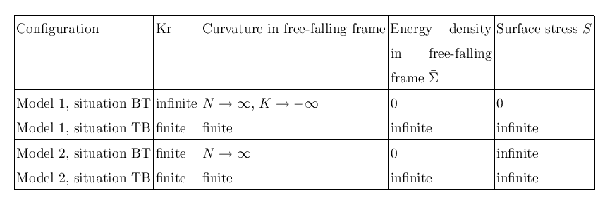
As an overall conclusion for the situation TB in Models 1 and 2, we find the results agree for both models. This can be explained and generalized as follows. Since, in the situation TB, the limit $\varepsilon\rightarrow 0$ is taken first, the dependence of the metric on $\varepsilon$ drops out in the final expressions for the curvature and surface stresses, so any model gives the same result. In addition, assuming that for $\varepsilon=0$ one has $\exp(2\Phi)=V$, and taking into account that $V(r_{+})=0$ and $\exp\left(\Phi(r_{+},\varepsilon)\right)\neq 0$, we obtain immediately from (14) that in the situation BT, $\bar{\Sigma}=0$, and in the situation TB, $\bar{\Sigma}$ diverges. This holds independently of the kind of the model used. Thus, a free-falling observer encounters diverging surface energy density in the situation TB. The same conclusion applies to the flux $J=S_{\mu\nu}\bar{u}^{\mu}\bar{n}^{\nu}$. In the non-extremal cases just studied, it turned out that each of the limits under discussion is singular: either the Kretschmann scalar or surface stresses on the throat (or both) diverge. Thus, the limit is singular. In other words, a black hole mimicker made from a wormhole, and in particular a black hole foil, is not smooth. It is convenient to summarize the results in a table shown in Figure 1.

Although the singular or almost singular behavior of these black hole mimickers based on $\varepsilon$-wormholes casts doubts on their real existence, it is worth our while to study a little more on the effects of such mimickers on infalling sources and their detection by far away observers. Intuitively it is clear that there should be some observational effects if infalling sources are distorted by stronger than normal tidal fields.

In Section III.1 on wormholes on the basis of nonextremal $\varepsilon$-metrics with surgery, we have discussed wormhole configurations which mimic non-extremal black holes. Here we consider the one-parametric deformation (1) such that for $\varepsilon=0$ our metric represents the gluing of two extremal Reissner-Nordstöm black holes. Note that in the non-extremal case, when using metric (1) we have chosen a function $V$ which itself does not contain the parameter $\varepsilon$. However, now such a simple construction cannot be implemented. Our goal is to trace the relationship between a wormhole metric with a generic $\varepsilon$ parameter ($\varepsilon\neq 0$), and a black hole metric ($\varepsilon=0$). If we start from equation (1) with $r_{+}=r_{-}$, i.e., $V=(1-\frac{r_{+}}{r})^{2}$, we encounter the immediate difficulty that spacetime is geodesically complete and represents an infinitely long horn, so one cannot speak about a wormhole at all. Therefore, we should deform the extremal Reissner-Nordström metric in a somewhat different way and include the parameter $\varepsilon$ not only into the function $\Phi$ but into $V$ as well. Let us make the simplest choice for $V(r,\varepsilon)$, namely,

$\delta(\varepsilon)$ being such that $0\leq\delta(\varepsilon)\leq 1$, and $\delta(0)=0$. At some $r_{0}>r_{+}$, we glue two copies of the spacetime, the “$+$” branch to the “$-$” branch. Then, the behavior of $K$ and $S$ follows from Eqs. (17) and (18). Note that if $\delta=\mathrm{constant}$ and $\delta\leq 1$ we return to the deformed non-extremal Reissner-Nordström case and the results (21)-(22) are reproduced, $\delta=1$ being the Schwarzschild case.

Using (16), i.e., $\exp(\Phi)=\sqrt{V+\varepsilon^{2}}$, and (37), we can study Model 1 in the extremal case.

Situation BT: As for the general behavior one finds,

and,

Let us analyze the naked behavior. In principle, the quantity $\alpha$ may be finite or infinite depending on the model for $\delta(\varepsilon)$. From Eq. (38), longitudinal contraction is finite if $\alpha$ is finite, or infinite if $\alpha$ is infinite. The value of $\bar{N}$ which determines transverse deformation can be found from eq. (19). Then, we obtain that in the limit under discussion

where $\beta=\lim_{\varepsilon\rightarrow 0}\frac{\delta}{\varepsilon^{2}}$. Then we have transverse stretching which is finite if $\beta$ is finite, or infinite if $\beta$ is infinite. The stress component $\bar{\Sigma}$ is finite, indeed zero, in the limit.

Situation TB: As for the general behavior one finds,

Note that when $\alpha=4$ in the situation BT, the quantities $K$ for two situations coincide. Let us analyze the naked behavior. Here there is finite longitudinal contraction, and no transverse deformation since, according to eq. (19), $\bar{N}\rightarrow 0$ in the limit under consideration. Thus, the only manifestation of naked behavior is connected with the surface stresses. According to (14), the quantity $\bar{\Sigma}$ behaves as

i.e., it diverges in situation TB.

Using Eq. (27), i.e., $\exp(\Phi)=\lambda\sqrt{V}+\varepsilon$, and (37), we can study Model 2 in the extremal case.

Situation BT: As for the general behavior one finds,

Let us analyze the naked behavior. There is no deformation in the radial direction. The behavior of $\bar{N}$ which is responsible for transverse deformation, can be obtained from (30) and coincides with (40) in the limit under discussion. Thus, again transverse stretching is finite if $\beta$ is finite, or infinite if $\beta$ is infinite. Note that it follows from the definitions of $\alpha$ and $\beta$ that $\alpha=\lim_{\varepsilon\rightarrow 0}\beta\delta$. According to the definition (37) of $\delta(\varepsilon)$, $\lim_{\varepsilon\rightarrow 0}\delta(\varepsilon)=0$. Therefore, if $\beta$ is finite, $\alpha=0$, then $K$, $S$, $\bar{N}$ and $\bar{\Sigma}$ are finite (moreover, $S=\bar{\Sigma}=0$), so naked behavior is absent in this case. On the other hand, as $\beta=\lim_{\varepsilon\rightarrow 0}\frac{\alpha}{\delta}$, in case $\alpha\neq 0$ the quantity $\beta$ diverges and so does $\bar{N}$. This means transverse stretching is infinite.

Situation TB: As for the general behavior one finds,

Let us analyze the naked behavior. One finds, finite contraction in the longitudinal direction and no transverse deformation. However,

i.e., it diverges.

As an overall conclusion, assuming that for $\varepsilon=0$, one has $\exp(2\Phi)=V,$ and taking into account that $V(r_{+})=0$, $\exp[\Phi(r_{+},\varepsilon)]\neq 0$, we obtain immediately from (14) that in the situation BT, $\bar{\Sigma}=0$, and in the situation TB, $\bar{\Sigma}$ diverges. This holds independently of the kind of the model, and is valid for the non-extremal spacetimes, as well as for the extremal spacetimes. Thus, a free-falling observer encounters diverging surface energy density in the situation TB. The same conclusion applies to the flux $J=S_{\mu\nu}\bar{u}^{\mu}\bar{n}^{\nu}$.

One essential feature of the almost extremal configurations under discussion consists in that we deal with shells which are timelike but become light-like in the limit when they are approaching the would-be horizon. A natural question arises: what happens if we start out our analysis with two extremal black hole spacetimes, i.e., putting $\varepsilon=0$ and $r_{0}=r_{+}$, and the shell in-between the two spacetimes lies on the event horizon and so is lightlike? More precisely, we are interested whether the stresses on the shell remain finite or become infinite. One can expect from our previous results that they are finite but this is not so obvious in advance. We have seen already that taking different limiting procedures in the near-horizon limit is a rather delicate issue. Moreover, the formalism for lightlike shells [19, 20] somewhat differs from that for timelike ones, so we perform our analysis anew. We restrict ourselves to the case of taking two extremal Reissner-Nordström black holes. The reason for this choice is that only extremal black holes are good candidates for gluing without severe singularities, i.e., the gluing procedure maintains a finite Kretschmann scalar throughout the spacetime as well as finite stresses on the glued surface. This case is also a Majumdar-Papapetrou case, and could be analyzed in the next section as well, but since it is also a limit of what has been done above, namely the null limit of a timelike wormhole throat with two extremal external vacuum spacetimes, we discuss it now. To match two extremal Reissner-Nordström spacetimes at the light-like surface $r_{0}=r_{+}$ we follow the general formalism for light-like shells [19, 20]. We write the metric in Kruskal-type coordinates $ds^{2}=-H(U,V)\,\,dUdV+r^{2}(U,V)\,\,(d\theta^{2}+\sin^{2}\theta d\phi^{2}).$ Let the surface $r_{0}=r_{+}$ correspond, say, to $U=0$. Then, the effective energy density is $\mu=-\frac{\gamma_{\theta\theta}}{16\pi r^{2}}$, (see, e.g., equation (3.99) of [19]). Here $\gamma_{\theta\theta}=[\left(\frac{\partial g_{\theta\theta}}{\partial x^{\alpha}}\right)_{+}-\left(\frac{\partial g_{\theta\theta}}{\partial x^{\alpha}}\right)_{-}]N^{\alpha}$, where the indexes $``+"$ and $``-"$ refer to the different sides of the shell, and the null vector $N^{\alpha}$ is such that $k_{\alpha}N^{\alpha}\neq 0$, with $k^{\alpha}$ being a null tangent vector. Now, the only nonvanishing components of $k^{\alpha}$ and $N^{\alpha}$, are by construction $k^{V}$ and $N^{U}$. Since there is no rest frame in the null case, the measured energy density $\mu$ depends on the chosen observer. To check that it is finite and non-zero, it is sufficient to check that $[\left(\frac{\partial r}{\partial U}\right)_{+}-\left(\frac{\partial r}{\partial U}\right)_{\_}]$ is finite and non-zero. For this purpose, it is sufficient to exploit the result of [21] where it is shown that $\frac{\partial r}{\partial U}=-1$ on the horizon. In our case, as we deal with two black holes instead of a single one, the coordinate $r$ increases on both sides of the shell. Thus, $\frac{\partial r}{\partial U}$ has different signs and takes the values $\pm 1$ on each side. So indeed, the difference is equal to $2$ and is finite and non-zero. In general, there are other contributions to the effective stress-energy tensor of the shell due to effective pressures and currents, but it is easy to show that in our case they are absent. It is worth noting that the gluing in our case differs from the gluing between different extremal Reissner-Nordström black holes considered in [22], in that we replaced the usual metric inside the horizon by their $``-"$ branch. It also differs from the wormhole construction used in [23] where two spheres were cut out from a vacuum Majumdar-Papapetrou system, or more precisely, they were cut from a single spacetime containing two extremal Reissner-Nordström black holes.

As a by-product of this light-like shell construction, and a very interesting one, we have just found a configuration that represents a regular wormhole configuration which is also a black hole. More important perhaps, in addition, it can serve as a classical model for an elementary particle in that (i) the system is characterized by a minimum number of fixed parameters like mass and charge and (ii) it is free of a central singularity inside. We are aware that it is not entirely of electromagnetic nature because it has stresses on the horizon, a kind of Poincaré stresses. But, anyway, such a surface stress, can be considered as a mild singularity when compared to the usual central singularity. In this model a free-falling observer can penetrate to the inside but, of course, cannot return back to the original asymptotic region, due to the existence of a horizon. So the wormhole is an untraversable one. Thus, the body under discussion combines features of an untraversable wormhole and a regular black hole, and can be called a worm-black hole. Since the proper distant to the extremal horizon is infinite, such a hybrid construction is similar to the null wormholes, or N-wormholes for short, see [24]. Note that it differs from configurations representing quasi-black holes. For example, in some quasi-black hole models, see [5], there is a region $r\leq r_{+}$ which becomes degenerate in the quasihorizon limit. This region is missing in our worm-black hole model, since the black hole metric beyond the horizon is replaced by a branch with an areal radius that grows away from the horizon. It also differs from the model considered in [21] where the external Reissner-Nordström part was glued to the Bertotti-Robinson metric that leads to surface stresses that vanish in the horizon limit in the static frame but grow unbound in the free-falling one, and as a result, the inner region becomes impenetrable for a free-falling observer (see [5] for details).

Bonnor stars are Majumdar-Papapetrou matter systems with either a sharp or smooth boundary to an exterior vacuum. Since Bonnor stars are paradigmatic to understand the formation of quasi-black holes (see [5]), it is interesting to use those stars on the threshold of forming a quasi-black hole to understand whether wormholes on the basis of quasi-black holes which can be formed from Bonnor stars, can mimic extremal black holes or not. This is an interesting variant, although with similarities, to wormholes on the basis of extremal $\varepsilon$-metrics. We use Bonnor stars, both in their compact version [25, 26], as well as in their extended one [27].

Now, we start from the configuration which contains Majumdar-Papapetrou matter inside and vacuum outside, a compact Bonnor star [25, 26]. Let us have a compact object, a Bonnor star, with extremal dust for $r\leq r_{0}$, joined to an extremal Reissner-Nordström metric for $r\geq r_{0}$. The potential $V(r)$ can be written as

with the mass density $\rho$ and the function $\mu(r)$ being connected through $4\pi\rho=\frac{\mu^{\prime}}{r^{2}}\left(1-\frac{\mu}{r}\right)$. The function $\mu(r)$ can be interpreted as the proper mass enclosed within a sphere of a radius $r$. In addition, for extremal dust, one has $\mu(r)=e(r)$, where $e(r)$ is the electric charge within this sphere. At the boundary $r_{0}$, one has $\mu(r_{0})=M$, and $e(r_{0})=Q$, such that $M=Q$, $M$ and $Q$ being the total mass and charge, respectively.