Volume Modulus Inflation and the Gravitino Mass Problem
Abstract:
The Hubble constant during the last stages of inflation in a broad class of models based on the KKLT mechanism should be smaller than the gravitino mass, . We point out that in the models with large volume of compactification the corresponding constraint typically is even stronger, , in Planck units. In order to address this problem, we propose a class of models with large volume of compactification where inflation may occur exponentially far away from the present vacuum state. In these models, the Hubble constant during inflation can be many orders of magnitude greater than the gravitino mass. We introduce a toy model describing this scenario, and discuss its strengths and weaknesses.
1 Introduction: Inflation and the Gravitino Mass
A realistic model of the universe should be consistent with all constraints, not just from high energy physics experiments but also from cosmological observations. Inflation is the leading scenario for the early universe and low-energy supersymmetry is the leading proposal for new physics subject to experimental test at the LHC. It is therefore important to develop models capable of including both these desirable features of physics beyond the standard model.
Many recent attempts to implement inflation in the context of string theory are based on the KKLT mechanism of vacuum stabilization [1] and its generalizations [2]. Until very recently, the standard assumption of many of these inflationary models was that inflation is a very high energy scale phenomenon, and therefore one can construct inflationary models quite independently of the requirements of the low-energy SUSY phenomenology.
However, recent studies of inflationary models in string theory revealed a rather unexpected fact: in the simplest models based on the KKLT mechanism the Hubble constant should be smaller than the present value of the gravitino mass [3],
| (1) |
The reason for this bound is that the gravitino mass at the supersymmetric KKLT minimum, with before the uplifting, is given by . Uplifting of the AdS minimum to the present nearly Minkowski vacuum occurs by adding to the potential a term of the form , where is the volume modulus and for a generic compactification and for the highly warped throat geometry. Since the uplifting is less significant at large , the energy barrier to decompactification created by the uplifting is generically slightly smaller than : . However, the volume modulus couples to all sources of energy due to the Weyl rescaling always present when deriving the 4-dimensional action. In particular, the energy of the inflaton field will give an additional uplifting of a similar type: . As this is also proportional to an inverse power of the volume modulus, it is larger at the minimum of the KKLT potential than at the top of the barrier. Therefore adding a large vacuum energy density to the KKLT potential, as required for inflation, may destabilize the minimum by uplifting it to a height greater than the height of the barrier, see Fig. 1. In typical KKLT-type models this leads to vacuum destabilization if the added energy density , which is responsible for inflation, is much greater than the height of the barrier . Since , this leads to the bound (1) (see [3] for a more detailed discussion of this issue, while a similar problem in a slightly different context was also found in [4]).
In KKLT-based models, it therefore seems that for a gravitino mass the Hubble constant during the last stages of a string theory inflation model should be quite low, TeV, which is ten orders of magnitude below the often discussed GUT inflation scale. Therefore if one believes in standard SUSY phenomenology with TeV, one should find a realistic particle physics model where the nonperturbative string theory dynamics occurs at the LHC scale or even lower (the mass of the volume modulus in the KKLT scenario typically is not much greater than the gravitino mass), and inflation occurs at a density at least 30 orders of magnitude below the Planck energy density [3]. For a recent analysis of this issue see e.g. [5] and for a discussion in the context of the heterotic string see [6].
This problem is quite generic. For example, recently a new interesting mechanism of moduli stabilization was proposed, which is based on the models with compacification on Nil manifolds with negative curvature [7]. This mechanism presents a significant modification of the compactifications on flat Calabi-Yau spaces, as suggested by the assumption of the low scale supersymmetry. And yet, the same constraint remains valid for the inflationary models in this scenario [8].
The situation becomes even trickier in the large volume models of vacuum stabilization [2]. In such models the height of the barrier is much smaller, . In this case, the constraint that the inflaton potential should not be much greater than the height of the barrier leads to the bound (in units )
| (2) |
For TeV this inequality implies that the Hubble constant during inflation in this class of models [9, 10] cannot exceed KeV, which is an extremely strong constraint.
There do exist proposals of low-scale inflationary models, for example the so-called MSSM inflation, which may occur for GeV or even for MeV [11]. Ref. [12] also contains a discussion of models where inflation may occur at extremely low scales, with an example of a model for which eV. In particular, if the inflaton potential energy at KeV could instantly transfer to thermal energy, the corresponding temperature would be about GeV, which is much greater than the critical temperature of the phase transition in the standard model. If this instantaneous transition is achievable, the temperatures would then be sufficiently high for the subsequent generation of a baryon asymmetry.
One can find models with a very low-scale inflation in the context of the KKLT or large volume scenarios, since the energy scale is exponentially sensitive to the parameter of the nonperturbative superpotential [1]. However, models of this type are very non-traditional, and their parameters are substantially different from the parameters of all current existing models of string theory inflation. Furthermore, as the required value of the slow-roll epsilon parameter is given by , low-scale inflation substantially increases the amount of fine-tuning required in the inflaton potential. It is important to know whether this tension between high-scale inflation and TeV supersymmetry is unavoidable or whether it is simply a consequence of the assumptions used so far in inflationary model-building.
This is not the first time that string theory and supergravity have encountered cosmological problems associated with the small value of the gravitino mass and of the moduli fields. The famous gravitino problem and the cosmological moduli problem are haunting us for more than two decades [13, 14, 15]. Now we see that the smallness of the gravitino mass leads to an additional problem in the context of string cosmology [3, 4]. This problem would disappear if one would consider supersymmetric models with large gravitino mass, for example [16, 17], or used a solution to the hierarchy problem different to that of TeV supersymmetry.11 1 For other problems with high values of the Hubble constant in string inflation see [18].
There exist ways to address this problem without increasing the value of the gravitino mass. For example, one may consider KKLT models with the racetrack superpotential containing at least two exponents and find parameters such that the supersymmetric minimum of the potential, even prior to uplifting, occurs at zero energy density [3], which would mean . By a slight change of parameters in this class of models, which are sometimes called KL models, one can get a gravitino mass that is nonzero but still much smaller than the height of the barrier, removing the constraint . In particular, one can use the KKLMMT brane inflation model [19, 20, 21, 22, 23, 24, 25] and implement it in the context of the KL scenario with .
The difficulty with this solution is that if we want to have many orders of magnitude greater than TeV, we need to fine-tune the parameters of the model to a corresponding accuracy. The origin of the electroweak scale is then a kind of accident, reducing the attractiveness of supersymmetric solutions to the hierarchy problem. However, this class of models has certain advantages from the point of view of vacuum stabilization [3], so it might happen that the required fine-tuning is not unreasonable.
Another possible solution of this problem was recently proposed in [26] in the context of the volume modulus inflation in the KKLT scenario. This model extended the KL model to involve triple gaugino condensation in the superpotential and also required a modification of the Kähler potential. It introduces 6 new parameters (two real parameters and two complex ones), and fine-tuned three of these parameters with accuracy ranging from to . This clearly demonstrates that it is quite difficult to avoid the constraint in such models, but nevertheless it is encouraging that it is possible to do so.
In this paper we will concentrate on the models with large volume of compactification [2] and propose another possible resolution of the gravitino mass problem, aiming at making a transition of scales from to natural. We shall discuss our idea and certain issues associated with it in the next sections.
2 Disentangling and : the basic idea
The idea we revisit in this paper is the assumption used so far in building supergravity models of inflation that the true minimum of the scalar potential is relatively close in field space to the locus at which inflation ends. We instead propose that inflation should end with a runaway in field space, with the true minimum lying a very long distance in field space from the location where inflation occurs (with the model discussed below, the distance in canonically normalized field space will correspond to approximately twenty Planckian distances). The problem we are trying to address is that characteristic inflationary energy scales are much larger than those appropriate for supersymmetry breaking. The advantage of a runaway epoch is that evolution along runaway potentials (e.g. of the form ) is one of the few efficient ways of naturally dissipating large quantities of energy and reducing the scale of the potential by many orders of magnitude. If the true minimum of the scalar potential lies a long way along the runaway direction, it naturally has much lower characteristic energy scales than apply during inflation.
In this case supergravity models of high-scale inflation consistent with low-scale supersymmetry breaking, in vacuo, should have three stages. In the first, inflation occurs at high energy scales with during inflation. In the second, inflation ends with the fields fast-rolling towards a runaway direction. For example, in the model below this is due to inflation occurring near an inflection point in the volume direction. As inflation ends it is necessary that trace quantities of radiation be generated to act as a seed for an attractor solution. In the third stage, the presence of small initial quantities of radiation drives the fields to an attractor solution. The attractor solution applies during the runaway epoch and dissipates energy. The scaling nature of the attractor solution avoids overshooting and guides the fields into the global minimum of the potential in which .22 2 For a recent discussion in the context of M-theory compactifications of the overshooting problem and how to avoid it, see [27]. This scenario is illustrated in Fig. 2.
The justification for the existence of a minimum at very large values of the volume, far along the runaway direction, is the large volume scenario [2], where the inclusion of corrections into the KKLT framework generates a new minimum of the scalar potential at exponentially large values of the volume, with hierarchically small values of .

To illustrate this idea, we start by studying moduli evolution in the following toy model describing a field with a potential
| (3) |
The particular form of this potential is motivated by that arising as the effective potential for the volume modulus in the large volume models. The connection to the large volume models and the supergravity origin of the above potential will be discussed in the next section. The 1-modulus potential (3) will not represent a complete model but will allow us to capture several key features of our proposal.
In (3) is the canonically normalized volume modulus, with , so is the volume of a 4-cycle. The first two terms of the potential correspond to the effective F-term potential for the volume modulus in the large volume models. The structure of these terms generates a minimum at large values of , . The definition of as implies that this is equivalent to the existence of a minimum at exponentially large volumes. As in string theory the gravitino mass is given by , where is the constant (flux) superpotential, hierarchically large volumes corresponds to hierarchically low gravitino mass. The final term, depending on , is the uplift term needed to lift the minimum of the potential to Minkowski space.
The second and third terms, depending on and , are only important at small volumes. These terms are not derived from string theory but are included in a phenomenological fashion in order to generate an inflection point, and thus inflation, at small volume. Besides the large volume minimum, occurring for large values of for which the and terms are irrelevant, by tuning and 33 3 Notice that in full string compactifications, corrections to the Kähler potential such as may generate the parameters will be functions of both fluxes and complex structure moduli and so would be expected to take on many possible values in the landscape. this sum of exponentials can have a non-monotonic shape for relatively small values of the field .
We will consider the following set of parameters, which are determined by the requirement of obtaining inflation satisfying the constraint which follow from the existing observational data: , , , , . The shape of the potential for this parameters at small is shown in Fig. 3. As we see, it has an inflection point at , where inflation takes place. The Hubble constant at that time is about GeV.
The potentials of this type have been used by many authors, see e.g. [28, 11, 21, 22, 23, 24, 25, 29, 30]. The typical feature of this class of models is that by tuning their parameters, the potential can always be represented as a sum of a linear term and a cubic term in a vicinity of the inflection point,
| (4) |
Here is the position of the inflection point. (In our case, , in Planck units.) The numerical values of are determined by fine-tuning of the values of the parameters in our full expression for . By making the linear term as small as possible, one can maximize the exponential growth of the universe during inflation, which may serve as a possible justification of the fine-tuning of the potential required for a long stage of inflation [29].
In the case where inflation is dominated by the cubic term, inflation starting at the inflection point is eternal, the spectral index , and the amplitude of perturbations of metric produced during inflation satisfies the COBE-WMAP normalization for
| (5) |
in units of Planck density [29]. We calculated and and tuned the parameters of our potential to satisfy this constraint and make vanishingly small. (If one reduces the degree of fine-tuning and considers a theory with a non-vanishing negative , one can significantly increase , but it will simultaneously decrease the degree of expansion of the universe during inflation [29].)
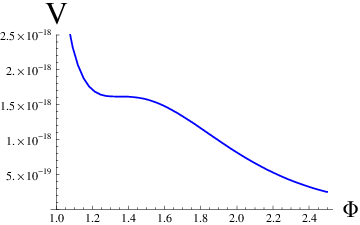
After inflation, the field enters a runaway period until it is captured by the minimum at , see Fig. 4. The parameters of our model were tuned to make the vacuum energy nearly zero in the minimum, and to have the gravitino mass there in the TeV range, . This last statement assumes that the gravitino mass is determined entirely by the volume, taking as usually done in the large volume models of moduli stabilisation.

Let us study the cosmological dynamics of rolling moduli in the potential (3). The and terms are only important at small and are highly suppressed for large . Conversely, the and terms only become important at large . These generate the minimum at exponentially large volumes and uplift it to Minkowski space. However, for smaller values of the volume these terms contribute highly subleading corrections to the potential. The upshot is that for a very large range of the volume the dominant term in the potential (3) is simply
| (6) |
with canonically normalized. In this regime the cosmological dynamics reduces to that of a pure exponential potential.
Evolution along runaway directions of this type is associated with the overshoot problem [31] and it is necessary that the fields are able to locate the global minimum of the potential. In the presence of any additional sources (such as radiation) exponential potentials have attractor solutions in which the different components of energy track the total energy as a constant fraction. This attractor solution can guide the fields to the global minimum without overshooting. In order to avoid decompactification and the overshooting problem, it is necessary that a small component of radiation be present in the evolution equations. We study the evolution with radiation present immediately at the end of inflation.44 4 A deficiency of the 1-modulus potential is that there is no way to generate this radiation, as any primordial radiation is diluted during inflation, and thus it has to be introduced by hand. With more complicated models, for example the 2-modulus case studied in the next section, there are ways to generate radiation at the end of inflation.
The evolution of fields in pure exponential potentials (6) has been studied for a long time. Naively will rapidly roll down the exponential slope into a kination phase. However in the presence of a background fluid, such as radiation, this does not occur [32, 33, 34, 35, 36, 37, 38, 39]. Since kinetic energy density falls faster than density of radiation,
the radiation comes to dominate the energy density, contributing additional Hubble friction to the field dynamics. The late-time attractor is a scaling solution in which the different components (radiation, potential energy, kinetic energy) constitute fixed fractions of the overall energy density.
Following [32, 34], the equations of motion are conveniently formulated in terms of the variables and defined by
and equal and respectively. It is also convenient to use as the time variable. The equations of motion are
| (7) | |||||
| (8) | |||||
| (9) | |||||
| (10) |
for radiation and for matter. For an exponential potential with , there exists a scaling solution given by [35, 33, 32]
For the case at hand of and , the attractor solution is
| (11) |
In the presence of any initial radiation or matter, this solution is the late-time attractor.
Considering the full potential (3), the attractor solution will exist so long as the pure exponential provides a good approximation to the potential. At small , this approximation will hold soon after inflation has ended, once the and terms become negligible. Inflation occurs at , corresponding to . At large , the attractor solution disappears as approaches the susy breaking vacuum and additional terms become important. We want the vacuum to satisfy , and as the characteristic scale of the large-volume potential is is (assuming ), this is attained when , see Fig. 4.
The regime in which the potential is well described by (6) and the attractor solution is valid is therefore
| (12) |
a range of almost twenty Planckian distances. We note that despite the substantially trans-Planckian field range, the potential is under good control: the high-scale theory is understood and the potential is simply a decompactification potential.
The physical minimum exists at , shortly followed by a local maximum representing the barrier to decompactification. In this regime the attractor solution is no longer present. It is necessary that the fields fall into the minimum rather than passing over the barrier and running away to decompactification. Whether this occurs or not depends on whether or not the field has located the attractor solution while in the range (12). If the attractor solution has been found, overshooting does not occur and settles into its minimum. This is illustrated in figure 5, which shows the behavior of the attractor solution as it approaches the minimum.

Whether or not the fields locate the attractor solution depends on the initial conditions and in particular the initial amount of radiation present. This is illustrated in figure 6. The initial conditions were chosen to be with varying initial values of . As expected, the larger the initial value of the more rapidly the attractor solution is found. As long as the attractor solution is found before the field reaches the decompactification barrier, overshooting does not occur. It is seen that even very small initial values of are sufficient to avoid overshooting, with even being sufficient to prevent overshooting.
This can be compared with the results of [37, 34] (see in particular figure 3 of [34]), where a similar question was studied in the context of a KKLT model, and to avoid overshooting was required across the whole range of parameter space.
In the case studied here it is much easier to avoid overshooting, which can be achieved with . It is easy to understand why this model is more efficient at avoiding overshooting than the models studied in [1, 34]. If the runaway direction comes from gaugino condensation in either the dilaton or volume directions, then the canonically normalized potential is a double exponential (as the potential is and the canonically normalized field is ). This is much steeper than the single exponential () present here, and so it is much harder to avoid overshooting.
The above one-field model has illustrated the required form of the potential, with a region suitable for inflation at small volume, a minimum at very large values of the volume, and a region in-between where the potential is described by a runaway. In order to locate the attractor solution that will guide the field to the global minimum, it is necessary that a small amount of matter or radiation can be generated as runaway starts. An attractive feature is that the quantity of radiation required for the fields not to overshoot is very small (). However, any primordial radiation will be diluted away during inflation. It is therefore necessary to extend the 1-modulus model to describe (partial) reheating and the generation of radiation at the end of inflation, as this is necessary to act as a source for the attractor solution.
3 Two-Field Inflation
We now consider a 2-field model which will justify the form of the potential used in the discussion of the 1-field model. The model we use is the following supergravity theory
| (13) |
Except for the parameters and , this is the supergravity theory that describes the large-volume models for compactifications on the Calabi-Yau manifold [2]. and are Kähler moduli: controls the size of the Calabi-Yau, whereas is the size of a small blow-up ‘hole’ in the Calabi-Yau.
Although all input parameters are of order unity, this theory admits a vacuum at exponentially large values of the volume with hierarchically small supersymmetry breaking [2]. In (13) additional corrections parametrized by and have been included. These are motivated by the existence of higher corrections to the Kähler potential, which will correct the Kähler potential at higher orders in the inverse volume expansion. As discussed above, these are not derived from string theory but are included in a phenomenological fashion to ensure an inflection point in the volume direction giving inflation at small volumes. In this respect the detailed form of these terms is not important - any other terms producing similar physics are equally acceptable.
We first explain the relation between the model of (13) and the 1-modulus example discussed in the previous section. We shall work at large volume, in the regime of parameter space that applies during the runaway period, and start by dropping the and terms of equations (13), which rapidly become irrelevant at large values of the volume. We also drop terms suppressed by higher orders in volume. It is in this region that the 1-modulus model is a precise limiting case of the 2-modulus potential. The supergravity scalar potential for the large-volume model of (13) is
| (14) |
We have included an uplift term (parametrized by ) to ensure the physical minimum has vanishing cosmological constant.
There are two fields, and . These two fields have very different characteristic mass scales. Working in the vicinity of , we have (with ) [2]
| (15) |
As the scale of the potential is , it follows that . We stress that these relations hold in the large-volume regime of the potential, which will correspond to the runaway period after inflation has ended. In this regime it is therefore possible to integrate out the heavy field to generate a single-field potential for the volume modulus . This approximation will work with increasing accuracy as the volume increases, as the parametric separation between the masses of and becomes increasingly large. Now,
| (16) | |||||
We can use equation (16) to integrate out . Up to terms subleading in , this generates a potential
Relating to using we see that this potential indeed takes the form of the 1-modulus potential (3). The and terms generate higher corrections of order and , as appropriate to match onto (3). We emphasise that at smaller values of the volume, and in particular during inflation, the above procedure of integration out is not valid. In this regime the two potentials are qualitatively similar - in both cases there is an inflection point in the volume direction - but it is not the case that the one-modulus model arises as a strict limit of the 2-modulus model.
Having explained the relation of the 2-modulus model to the simpler 1-modulus case studied in the previous section, we now turn to the full two-field system described by (13). We use the following numerical parameters
The choice of numerical parameters is such that a minimum exists at exponentially large volumes with a TeV gravitino mass, while the energy scale during inflation is . As this model has various phenomenological difficulties, to be explained further below, we shall not attempt a detailed comparison with observation. The parameters and are chosen such that at smaller values of the volume there exists an inflection point in the volume direction. The large flux numbers present in flux compactifications (typically ) make the relatively large values of and not unreasonable. We choose the initial conditions so that fields start near the inflection point, where inflation will occur, ending with the volume rolling away from the inflection point towards a decompactification limit.
In addition to the volume direction, there is also the direction. As the corrections to the Kähler potential of (13) depend only on the volume, they do not induce a potential for the direction at constant volume. This direction is lifted only by non-perturbative superpotential terms and so is flat at large . This is equivalent to the method used to generate a flat inflationary direction in Kähler moduli inflation [9, 10]. In the vicinity of an inflection point for the volume direction, and with the direction lifted only by non-perturbative effects, the resulting potential is therefore flat and suitable for slow-roll inflation.55 5 There may be additional loop corrections in that would lift this flatness, but these are beyond the scope of this paper.
We choose initial conditions in which the fields have no initial velocities and have initial values
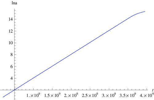
Figure 7 shows the evolution of the scale factor and figure 8 shows the evolution of the fields with time. For numerical reasons when performing the numerical integration we have restricted to the last ten efolds, but there is no conceptual difficulty in extending this to sixty efolds. In figure 9 we show the form of the field evolution. Inflation occurs early in the field trajectory, followed by a period of oscillations. The initial conditions used are chosen to ensure that as inflation ends there is runaway in the volume direction (the direction) and oscillations in the direction. The presence of oscillations ensures that some quantity of post-inflationary radiation will be generated by the decays of the oscillating field. The large fine-tuning of initial conditions is primarily due to the need to ensure oscillations, and thus radiation, are present at the end of inflation, as it is the radiation that allows the attractor solution to exist and be located. In the appendix we show that the tracker solution present in the 1-modulus case is also present in the 2-modulus case. Numerically, we can confirm that this is also an attractor. This radiation can act as a seed allowing the attractor solution to be located. It is the tracker solution that will guide the fields to the global minimum.

In figures 8 and 9 we see that with a purely classical evolution the magnitude of oscillations of grows with time. If the magnitude of oscillations is not sufficiently reduced by particle decays, then in fact the oscillatory field escapes from its stabilized location. In this case there is no way to find the global minimum of the scalar potential and the solution will decompactify. Particle decays are intrinsically quantum events and are not explicitly included in the numerical evolution shown in figures 6. If we assume a brane wrapping the cycle , then the direction couples to radiation through the Lagrangian terms
| (17) |
From this the decay width for can be computed [47],
| (18) |
Evaluating this for the model of 13, we have
The most important relation is the relative size of the decay width and the Hubble scale . The volume scaling of this is given by
The question of whether the decays reduce the oscillation amplitude sufficiently rapidly is determined by the model-dependent details of the coupling of to radiation and on the initial conditions. If necessary it is always possible to tune the initial conditions to ensure there are sufficient oscillations of the field in order to generate sufficient decays to radiation.
The most important point that this model illustrates is that inflation ends with runaway in the volume direction together with a small quantity of radiation. The radiation will serve as a seed for the attractor solution that will guide the fields into the global minimum. In the specific case of the model above the radiation is provided by decays of oscillations.
4 Conclusions and Challenges
Let us discuss what has been done in this paper and what remains to be done. This paper has proposed a mechanism in which high-scale inflation and low scale supersymmetry can coexist. The model discussed explicitly is by no means problem-free and should be regarded primarily as an illustration of the main features of the proposed mechanism. These involve a runaway at the end of inflation, with the true vacuum far away from that applicable during inflation.
Let us discuss some open questions for this explicit model. First, volume modulus inflation was obtained by fine tuning the parameters and to generate an inflection point. The amount of fine tuning is at a similar order to that required in models of brane-antibrane inflation but is not explicit as it relies on higher order quantum corrections to the Kähler potential that are not controlled. The use of the volume modulus for the inflaton was only for simplicity and it is an interesting challenge to improve the implementation of inflation. One interesting generalization would be to a hybrid model of inflation in which the decompactification direction that generates the runaway plays the role of the tachyonic field that ends inflation.
A second issue relates to the generation of radiation and isocurvature perturbations. In the inflationary regime, we had the inflaton (volume) modulus light to drive inflation but also required the second (small) modulus to be light. We also needed a large fine-tuning of the initial conditions. This was to ensure that the small modulus would oscillate at the end of inflation and generate through its decays the radiation necessary for the attractor solution. Indeed, if the second field is very heavy, it always follows the time-dependent position of its potential determined by the slowly-changing inflaton. In this case it will not experience oscillations after the end of inflationary stage, and so it would not be possible to generate the radiation required for the attractor solution.
The lightness of this modulus is a source of isocurvature perturbations that are highly constrained observationally. For the purposes of this paper, which aims simply at combining high scale inflation with TeV supersymmetry, this is less of an issue. To make our model fully realistic, one may consider the second field to be a curvaton and later on having the isocurvature perturbations converted to adiabatic perturbations [40]. Another possibility to use the second light field for generation of adiabatic perturbations is discussed in [41]. In both cases, inflation may produce perturbations of metric with a measurable degree of non-gaussianity. This can be a potential advantage of our model, having in mind the recent controversy with respect to the possible non-gaussianity in the WMAP data [43, 44, 45, 46].
On the other hand, the fact that both moduli are light in the inflation regime could be modified by additional quantum corrections to the Kähler potential. Such corrections are potentially a problem for Kähler moduli inflation as proposed in [9]. In that case the flatness of the potential for the small modulus is natural up to and including the leading corrections to the Kähler potential. String loop corrections [42] not included in [9] have the potential to lift that flatness. A correction of the form would give a dominant contribution to the mass of , resurrecting the problem for Kähler moduli inflation but avoiding the second light direction in our case.
All the above issues refer specifically to the particular inflationary model described in this paper. In general, for the proposed mechanism to occur the principal requirements on the inflationary model are only that at the end of inflation there is both a small amount of radiation present and runaway in the volume direction. In this respect the overall scenario is not tied to the particular model used in this paper. The requirement of radiation at the end of inflation is suggestive of models of brane inflation, where the brane annihilation that ends inflation will generate large quantities of radiation.
Finally, as generally holds for models of cosmology with TeV-scale supersymmetry, this scenario still suffers from the cosmological moduli problem [15]. This was recently re-analyzed in [47] for the large volume class of models. While the small moduli decay very rapidly, the volume modulus has an MeV-scale mass and gravitational strength interactions. It naturally decays very late in the history of the universe ruining successful nucleosynthesis. An often discussed solution of this problem is to have a late period of inflation to dilute the modulus, such as thermal inflation [48]. Even though an explicit realization of thermal inflation in our model is not at hand, the attractor solution automatically contains a high fraction of radiation at the end of the runaway period, which may provide the right initial conditions for thermal inflation.
Thus we see that in principle there exist various possibilities to avoid the bound in string cosmology. One of these possibilities is to study inflation in KL models [3], or in the model proposed recently in [26]. Yet another possibility is to construct a cosmological scenario along the lines outlined in this paper. However, none of these possibilities is easy and all of them require fine-tuning. This may just mean that the constraint is quite robust and hard to avoid, so one should consider inflationary models where inflation occurs on a very small energy scale.
It is worth emphasizing the fact that low-energy supersymmetry, especially within string constructions, tends to put very strong constraints on viable cosmological scenarios. The constraint is just one of them. Other constraints include the cosmological problems associated with light gravitino and moduli fields [13, 14]. These cosmological difficulties may lead us to reconsider how much weight to give to the supersymmetric solution of the hierarchy problem. As mentioned in the Introduction, one route out is to have models of high scale supersymmetry breaking. These automatically avoid the cosmological problems associated to the moduli fields and the gravitino but replace the standard solution to the hierarchy problem by appeals to anthropic considerations and string theory landscape. On the other hand we can take a positive view on the existence of so many cosmological constraints: they provide powerful guidelines for the properties of realistic models and eliminate many potential vacua that would be otherwise consistent. Fortunately, experimental evidence will soon tell us if low-energy supersymmetry is realized in nature in a long anticipated way.
If supersymmetry is indeed discovered at the LHC, it would falsify many proposed models of inflation in both string and field theory. It would then be of extreme importance to understand how low-scale supersymmetry can be consistent with the observational evidence for inflation at very high energy scales , particularly if tensor perturbations were observed by either WMAP or Planck. In this paper we have proposed that this can occur if inflation ends with runaway towards a decompactification direction. The energy scales during inflation and the energy scales can then be hierarchically different. As long as some radiation is present or generated at the end of inflation, an attractor solution can guide the fields into the global minimum of the potential, avoiding the cosmological overshoot problem. We have presented a model to illustrate this scenario, where the volume modulus was the inflaton and the runaway direction was towards the large volume minimum. The ultimate aim of model-building is to construct a model that is fully realistic when confronted with both cosmological and phenomenological data - our work is one step towards this goal.
Acknowledgments.
We thank M. Cicoli, E. Copeland, S. Sarkar, H. Tye and especially C.P. Burgess for interesting discussions. JC is funded by Trinity College, Cambridge and also thank the University of Texas at Austin for hospitality while some of this work was carried out. He was supported in part by NSF grant PHY-0455649. FQ is partially funded by STFC and a Royal Society Wolfson merit award and thank the Mitchell family and the organizers of the Cambridge-Texas A&M Cook’s Branch meeting. RK and AL were supported in part by NSF grant PHY-0244728. They are grateful for the hospitality and support extended to them at YITP, Kyoto.A: Tracker solution for two modulus model
In section 2 we studied the tracker solution in the presence of radiation for the single field potential that arises from integrating out the heavy mode. Here we show the existence of a tracker solution in the presence of radiation for the full two-modulus model with non-canonical kinetic terms. The tracker solution will apply after the end of inflation, namely during the runaway regime of the potential. The model is described by
Here we have used simply the potential arising for the large volume models, without the additional terms and that were only important at small volumes. Starting with a Lagrangian
| (19) |
the equations of motion for the complex fields are
| (20) | |||||
| (21) |
with the background (radiation) energy density and . We fix the axionic parts of and and write the equations solely in terms of the real parts and . The equations of motion are then
| (22) |
It is useful to rewrite the Friedmann equation (21) as
| (23) |
In a tracker solution the kinetic, potential and background energies are all constant fractions of the total energy. This implies , , and , giving
| (24) |
and so in any tracker solution
| (25) |
The assumption of a radiation background, for which , then implies and . As the magnitude of the potential is determined in terms of the compactification volume by , we can also deduce that
As at its minimum the direction has characteristic mass , we anticipate that in a tracker solution . We will show below that this assumption is self-consistent. From equation (16) this implies
| (26) |
We can now check that the above ansatz is consistent and indeed leads to a solution of the equations of motion.
Considering the leading terms at large volume, the Kähler potential gives the following Kähler metric
| (27) |
From this we can compute the Christoffel symbols
Using the above ansätze we evaluate
| (28) | |||||
| (29) |
We expect any tracker solution to be valid during the regime in which the potential is dominated by the third term (the correction). During this regime, . In the tracker solution, we also expect to have (as the heavy field should be fixed at its minimum). In this case,
| (30) | |||||
We have here used the assumption that . Comparison with equations (22) and (28) then gives
The equations of motion give
| (31) | |||||
Comparison with equation (22) and (29) then gives
| (32) |
Using , eq. (32) is satisfied so long as
| (33) |
Equation (33) can be solved to determine the precise value of in the tracker solution.
As this corresponds at leading order in to our ansatz (26), this shows that our approximations were self-consistent. As the characteristic scale of is itself, the requirement of (33) that is consistent with the interpretation that has been integrated out.
It is interesting to analyze the origin of the kinetic energy in the tracker solution. Writing
| (34) | |||||
we see that the kinetic energy of the solution is dominated by the motion of the light field () and that the contributions of the heavy field to the kinetic energy vanish at large . We can verify that the above results are consistent with the single-field attractor. We have
and so . This reproduces the attractor values of eq (11) for the single-field evolution. It is thus possible to explicitly solve the equations of motion for the 2-modulus model for the runaway regime in the presence of radiation, finding as expected the same tracker solution as seen when the heavy modulus is integrated out.
The tracker solution requires the presence of radiation - in the absence of radiation, the small field cannot be confined within its trough and the moduli evolution enters a kination phase which eventually leads to decompactification. Furthermore, the simple existence of the tracker solution does not imply that the moduli evolution will locate the tracker solution. To locate the tracker solution, sufficient radiation needs to be generated at the end of inflation to attract the moduli evolution into the tracker solution. Whether sufficient radiation can be generated or not is a dynamical question that depends on the amplitude of oscillations of the small field and on its couplings to matter - we saw in figure 9 that in a purely classical evolution, with no quantum decays, the small field cannot be confined within its trough.
As for the 1-modulus case, the tracker solution is (numerically) also found to be an attractor solution. If the fields can locate the attractor solution, then this will guide them through the runaway epoch and into the large-volume minimum without overshooting.
References
- [1] S. Kachru, R. Kallosh, A. Linde and S. P. Trivedi, “De Sitter vacua in string theory,” Phys. Rev. D 68 (2003) 046005 [arXiv:hep-th/0301240].
- [2] V. Balasubramanian, P. Berglund, J. P. Conlon and F. Quevedo, “Systematics of moduli stabilization in Calabi-Yau flux compactifications,” JHEP 0503, 007 (2005) [arXiv:hep-th/0502058]; J. P. Conlon, F. Quevedo and K. Suruliz, “Large-volume flux compactifications: Moduli spectrum and D3/D7 soft supersymmetry breaking,” JHEP 0508 (2005) 007 [arXiv:hep-th/0505076].
- [3] R. Kallosh and A. Linde, “Landscape, the scale of SUSY breaking, and inflation,” JHEP 0412, 004 (2004) [arXiv:hep-th/0411011]; J. J. Blanco-Pillado, R. Kallosh and A. Linde, “Supersymmetry and stability of flux vacua,” JHEP 0605, 053 (2006) [arXiv:hep-th/0511042]; R. Kallosh and A. Linde, “Testing String Theory with CMB,” JCAP 0704 (2007) 017 [arXiv:0704.0647 [hep-th]].
- [4] W. Buchmuller, K. Hamaguchi, O. Lebedev and M. Ratz, “Maximal temperature in flux compactifications,” JCAP 0501, 004 (2005) [arXiv:hep-th/0411109].
- [5] L. Covi, M. Gomez-Reino, C. Gross, J. Louis, G. A. Palma and C. A. Scrucca, “Constraints on modular inflation in supergravity and string theory,” arXiv:0805.3290 [hep-th].
- [6] Z. Lalak, G. G. Ross and S. Sarkar, Nucl. Phys. B 766, 1 (2007) [arXiv:hep-th/0503178].
- [7] E. Silverstein, “Simple de Sitter Solutions,” arXiv:0712.1196 [hep-th].
- [8] E. Silverstein and A. Westphal, “Monodromy in the CMB: Gravity Waves and String Inflation,” arXiv:0803.3085 [hep-th].
- [9] J. P. Conlon and F. Quevedo, “Kaehler moduli inflation,” JHEP 0601, 146 (2006) [arXiv:hep-th/0509012].
- [10] J. R. Bond, L. Kofman, S. Prokushkin and P. M. Vaudrevange, “Roulette inflation with Kaehler moduli and their axions,” Phys. Rev. D 75, 123511 (2007) [arXiv:hep-th/0612197]. Z. Lalak, D. Langlois, S. Pokorski and K. Turzynski, JCAP 0707 (2007) 014 [arXiv:0704.0212 [hep-th]]. R. Holman and J. A. Hutasoit, “Systematics of moduli stabilization, inflationary dynamics and power spectrum,” JHEP 0608 (2006) 053 [arXiv:hep-th/0606089]. A. Misra and P. Shukla, “Large Volume Axionic Swiss-Cheese Inflation,” arXiv:0712.1260 [hep-th].
- [11] R. Allahverdi, K. Enqvist, J. Garcia-Bellido, A. Jokinen and A. Mazumdar, “MSSM flat direction inflation: slow roll, stability, fine tuning and reheating,” JCAP 0706, 019 (2007) [arXiv:hep-ph/0610134]; A. Mazumdar, “New developments on embedding inflation in gauge theory and particle physics,” arXiv:0707.3350 [hep-ph].
- [12] G. G. Ross and S. Sarkar, “Successful supersymmetric inflation,” Nucl. Phys. B 461 (1996) 597 [arXiv:hep-ph/9506283]. G. German, G. G. Ross and S. Sarkar, “Low-scale inflation,” Nucl. Phys. B 608 (2001) 423 [arXiv:hep-ph/0103243].
- [13] P. Fayet, “Phenomenology Of Supersymmetry,” Talk at the XVIIth Rencontre de Moriond, Ecole Normale Superieure preprint LPTENS 82/10 (1982); S. Weinberg, “Cosmological Constraints On The Scale Of Supersymmetry Breaking,” Phys. Rev. Lett. 48, 1303 (1982); J. R. Ellis, A. D. Linde and D. V. Nanopoulos, “Inflation Can Save The Gravitino,” Phys. Lett. B 118, 59 (1982); L. M. Krauss, “New Constraints On Ino Masses From Cosmology. 1. Supersymmetric Inos,” Nucl. Phys. B 227, 556 (1983); M. Y. Khlopov and A. D. Linde, “Is It Easy To Save The Gravitino?,” Phys. Lett. B 138, 265 (1984).
- [14] G. D. Coughlan, W. Fischler, E. W. Kolb, S. Raby and G. G. Ross, “Cosmological Problems For The Polonyi Potential,” Phys. Lett. B 131, 59 (1983); A. S. Goncharov, A. D. Linde and M. I. Vysotsky, “Cosmological Problems For Spontaneously Broken Supergravity,” Phys. Lett. B 147, 279 (1984).
- [15] T. Banks, D. B. Kaplan and A. E. Nelson, “Cosmological implications of dynamical supersymmetry breaking,” Phys. Rev. D 49 (1994) 779 [arXiv:hep-ph/9308292]; B. de Carlos, J. A. Casas, F. Quevedo and E. Roulet, “Model independent properties and cosmological implications of the dilaton and moduli sectors of 4-d strings,” Phys. Lett. B 318 (1993) 447 [arXiv:hep-ph/9308325].
- [16] O. DeWolfe and S. B. Giddings, “Scales and hierarchies in warped compactifications and brane worlds,” Phys. Rev. D 67, 066008 (2003) [arXiv:hep-th/0208123].
- [17] N. Arkani-Hamed and S. Dimopoulos, “Supersymmetric unification without low energy supersymmetry and signatures for fine-tuning at the LHC,” JHEP 0506, 073 (2005) [arXiv:hep-th/0405159]; N. Arkani-Hamed, S. Dimopoulos, G. F. Giudice and A. Romanino, “Aspects of split supersymmetry,” Nucl. Phys. B 709, 3 (2005) [arXiv:hep-ph/0409232].
- [18] A. R. Frey, A. Mazumdar and R. C. Myers, “Stringy effects during inflation and reheating,” Phys. Rev. D 73 (2006) 026003 [arXiv:hep-th/0508139].
- [19] S. Kachru, R. Kallosh, A. Linde, J. M. Maldacena, L. P. McAllister & S. P. Trivedi, “Towards inflation in string theory,” JCAP 0310, 013 (2003) [arXiv:hep-th/0308055].
- [20] C. P. Burgess, J. M. Cline, H. Stoica and F. Quevedo, “Inflation in realistic D-brane models,” JHEP 0409 (2004) 033 [arXiv:hep-th/0403119].
- [21] D. Baumann, A. Dymarsky, I. R. Klebanov, L. McAllister & P. J. Steinhardt, “A Delicate Universe,” Phys. Rev. Lett. 99, 141601 (2007) [arXiv:0705.3837 [hep-th]].
- [22] D. Baumann, A. Dymarsky, I. R. Klebanov and L. McAllister, “Towards an Explicit Model of D-brane Inflation,” JCAP 0801, 024 (2008) [arXiv:0706.0360 [hep-th]].
- [23] A. Krause & E. Pajer, “Chasing Brane Inflation in String-Theory,” arXiv:0705.4682 [hep-th].
- [24] S. Panda, M. Sami and S. Tsujikawa, “Prospects of inflation in delicate D-brane cosmology,” Phys. Rev. D 76, 103512 (2007) [arXiv:0707.2848 [hep-th]].
- [25] N. Itzhaki and E. D. Kovetz, “Inflection Point Inflation and Time Dependent Potentials in String Theory,” JHEP 0710, 054 (2007) [arXiv:0708.2798 [hep-th]].
- [26] M. Badziak and M. Olechowski, “Volume modulus inflation and a low scale of SUSY breaking,” arXiv:0802.1014 [hep-th].
- [27] B. S. Acharya, P. Kumar, K. Bobkov, G. Kane, J. Shao and S. Watson, arXiv:0804.0863 [hep-ph].
- [28] R. Holman, P. Ramond & G. G. Ross, “Supersymmetric Inflationary Cosmology,” Phys. Lett. B 137, 343 (1984).
- [29] A. Linde and A. Westphal, “Accidental Inflation in String Theory,” JCAP 0803, 005 (2008) [arXiv:0712.1610 [hep-th]].
- [30] B. Underwood, “Brane Inflation is Attractive,” arXiv:0802.2117 [hep-th].
- [31] R. Brustein and P. J. Steinhardt, “Challenges for superstring cosmology,” Phys. Lett. B 302 (1993) 196 [arXiv:hep-th/9212049].
- [32] E. J. Copeland, A. R. Liddle and D. Wands, “Exponential potentials and cosmological scaling solutions,” Phys. Rev. D 57, 4686 (1998) [arXiv:gr-qc/9711068].
- [33] P. G. Ferreira and M. Joyce, “Cosmology with a Primordial Scaling Field,” Phys. Rev. D 58, 023503 (1998) [arXiv:astro-ph/9711102].
- [34] T. Barreiro, B. de Carlos, E. Copeland and N. J. Nunes, “Moduli evolution in the presence of flux compactifications,” Phys. Rev. D 72, 106004 (2005) [arXiv:hep-ph/0506045].
- [35] C. Wetterich, “Cosmology and the Fate of Dilatation Symmetry,” Nucl. Phys. B 302, 668 (1988).
- [36] N. Kaloper and K. A. Olive, “Dilatons in string cosmology,” Astropart. Phys. 1 (1993) 185. A. Albrecht, C. P. Burgess, F. Ravndal and C. Skordis, “Natural quintessence and large extra dimensions,” Phys. Rev. D 65 (2002) 123507 [arXiv:astro-ph/0107573].
- [37] R. Brustein, S. P. de Alwis and P. Martens, “Cosmological stabilization of moduli with steep potentials,” Phys. Rev. D 70, 126012 (2004) [arXiv:hep-th/0408160]. I. Ben-Dayan, R. Brustein and S. P. de Alwis, arXiv:0802.3160 [hep-th].
- [38] N. Kaloper, J. Rahmfeld and L. Sorbo, “Moduli entrapment with primordial black holes,” Phys. Lett. B 606 (2005) 234 [arXiv:hep-th/0409226]. A. Berndsen, T. Biswas and J. M. Cline, “Moduli stabilization in brane gas cosmology with superpotentials,” JCAP 0508 (2005) 012 [arXiv:hep-th/0505151]. N. Itzhaki and E. D. Kovetz, “Inflection Point Inflation and Time Dependent Potentials in String Theory,” arXiv:0708.2798 [hep-th].
- [39] D. A. Easson and M. Trodden, Phys. Rev. D 72 (2005) 026002 [arXiv:hep-th/0505098].
- [40] A. D. Linde and V. Mukhanov, “Nongaussian isocurvature perturbations from inflation,” Phys. Rev. D 56, 535 (1997) [arXiv:astro-ph/9610219]; K. Enqvist and M. S. Sloth, “Adiabatic CMB perturbations in pre big bang string cosmology,” Nucl. Phys. B 626, 395 (2002) [arXiv:hep-ph/0109214]; D. H. Lyth and D. Wands, “Generating the curvature perturbation without an inflaton,” Phys. Lett. B 524, 5 (2002) [arXiv:hep-ph/0110002]; T. Moroi and T. Takahashi, “Effects of cosmological moduli fields on cosmic microwave background,” Phys. Lett. B 522, 215 (2001) [Erratum-ibid. B 539, 303 (2002)] [arXiv:hep-ph/0110096].
- [41] G. Dvali, A. Gruzinov and M. Zaldarriaga, “A new mechanism for generating density perturbations from inflation,” Phys. Rev. D 69, 023505 (2004) [arXiv:astro-ph/0303591]; L. Kofman, “Probing string theory with modulated cosmological fluctuations,” arXiv:astro-ph/0303614; A. Mazumdar and M. Postma, “Evolution of primordial perturbations and a fluctuating decay rate,” Phys. Lett. B 573, 5 (2003) [Erratum-ibid. B 585, 295 (2004)] [arXiv:astro-ph/0306509]; F. Bernardeau, L. Kofman and J. P. Uzan, “Modulated fluctuations from hybrid inflation,” Phys. Rev. D 70, 083004 (2004) [arXiv:astro-ph/0403315]; D. H. Lyth, “Generating the curvature perturbation at the end of inflation,” arXiv:astro-ph/0510443; T. Matsuda, “Modulated Inflation,” arXiv:0801.2648 [hep-ph]; T. Suyama and M. Yamaguchi, “Non-Gaussianity in the modulated reheating scenario,” Phys. Rev. D 77, 023505 (2008) [arXiv:0709.2545 [astro-ph]]; M. Sasaki, “Multi-brid inflaton and non-Gaussianity,” in preparation.
- [42] M. Berg, M. Haack and B. Kors, “String loop corrections to Kaehler potentials in orientifolds,” JHEP 0511 (2005) 030 [arXiv:hep-th/0508043]; M. Berg, M. Haack and E. Pajer, “Jumping Through Loops: On Soft Terms from Large Volume Compactifications,” JHEP 0709 (2007) 031 [arXiv:0704.0737 [hep-th]]; M. Cicoli, J. P. Conlon and F. Quevedo, “Systematics of String Loop Corrections in Type IIB Calabi-Yau Flux Compactifications,” JHEP 0801, 052 (2008) [arXiv:0708.1873 [hep-th]]. M. Cicoli, J. P. Conlon and F. Quevedo, arXiv:0805.1029 [hep-th].
- [43] A. P. S. Yadav and B. D. Wandelt, “Detection of primordial non-Gaussianity (fNL) in the WMAP 3-year data at above 99.5% confidence,” arXiv:0712.1148 [astro-ph].
- [44] C. Hikage, T. Matsubara, P. Coles, M. Liguori, F. K. Hansen and S. Matarrese, “Primordial Non-Gaussianity from Minkowski Functionals of the WMAP Temperature Anisotropies,” arXiv:0802.3677 [astro-ph].
- [45] J. D. McEwen, M. P. Hobson, A. N. Lasenby and D. J. Mortlock, “A high-significance detection of non-Gaussianity in the WMAP 5-year data using directional spherical wavelets,” arXiv:0803.2157 [astro-ph].
- [46] E. Komatsu et al. [WMAP Collaboration], “Five-Year Wilkinson Microwave Anisotropy Probe (WMAP) Observations: Cosmological Interpretation,” arXiv:0803.0547 [astro-ph].
- [47] J. P. Conlon and F. Quevedo, “Astrophysical and Cosmological Implications of Large Volume String Compactifications,” JCAP 0708, 019 (2007) [arXiv:0705.3460 [hep-ph]].
- [48] D. H. Lyth and E. D. Stewart, “Thermal Inflation And The Moduli Problem,” Phys. Rev. D 53 (1996) 1784 [arXiv:hep-ph/9510204].