Critical adsorption and critical Casimir forces for geometrically structured confinements
Abstract
We study the behavior of fluids, confined by geometrically structured substrates, upon approaching a critical point at in their bulk phase diagram. As generic substrate structures periodic arrays of wedges and ridges are considered. Based on general renormalization group arguments we calculate, within mean field approximation, the universal scaling functions for order parameter profiles of a fluid close to a single structured substrate and discuss the decay of its spatial variation into the bulk. We compare the excess adsorption at corrugated substrates with the one at planar walls. The confinement of a critical fluid by two walls generates effective critical Casimir forces between them. We calculate corresponding universal scaling functions for the normal critical Casimir force between a flat and a geometrically structured substrate as well as the lateral critical Casimir force between two identically patterned substrates.
I Introduction
The confinement of a fluid which is close to its critical point at induces remarkable deviations from its bulk behavior. Typically, the boundary of a system affects the local structural properties of condensed matter within a layer of thickness of the bulk correlation length, which diverges upon approaching criticality as , where , is a standard bulk critical exponent, and are nonuniversal amplitudes above () or below () . For binary liquid mixtures, the disordered phase at is the one in which its two components are mixed, whereas in the ordered phase at there is phase separation in two phases being rich in one or the other component. (At lower critical points the disordered phase occurs for and the ordered ones at .) Accordingly, near the critical demixing point the scalar order parameter is a suitably defined concentration difference of the two species, belonging to the Ising universality class. The generic preference of a surface for either one of the two species forming the binary fluid amounts to the presence of an effective surface field which affects the order parameter profile close to the wall such that it is nonzero even in the disordered (mixed) phase for . Upon approaching , these so-called critical adsorption profiles, describing the concentration enhancement near the surface, become long ranged due to the divergence of the correlation length [1, 2, 3]. In the semi-infinite geometry the transitions from the phase in which only the region near a single surface is ordered to the one in which also the bulk is ordered are known as the so-called extraordinary or normal surface transitions [4, 5]. In the slab geometry the confinement of critical fluctuations of the order parameter gives rise to critical Casimir forces attracting or repelling the confining walls, which can be of significant strength [1, 6, 7, 8, 9, 10]. This is the thermodynamic analogue of the quantum-electrodynamic Casimir effect originating from the confinement of vacuum fluctuations [11, 12]. Critical adsorption has been investigated experimentally for flat substrates (see, e.g., Refs. 15, 13, 14, 16, 17 and references therein). Also, there is strong experimental evidence for the occurrence of critical Casimir forces [18, 19, 20, 21], and recently a direct measurement of the critical Casimir force between a wall and a colloid has been reported [22]. So far the theoretical investigations of critical adsorption and the critical Casimir effect have been focused on topologically flat surfaces (see, e.g., Refs. 2, 3, 13, 10, 24, 23) or curved surfaces and colloids (see, e.g., Refs. 25, 26, 27, 28, 29, 30).
Nowadays, experimental techniques are available which allow one to endow a solid surface with a precisely defined geometrical or chemical structure in the micro- and nanometer range (see, e.g., Refs. 31, 32, 33, 34). Chemically and geometrically structured substrates are of major importance for the construction of a ’lab on a chip’ [35]. Critical adsorption and critical Casimir forces for chemically structured but topologically flat confinements have been studied theoretically [36, 37]. Typical man-made geometrical structures are periodic in one direction and consist of grooves with wedge-like shapes. The effects of such roughness and of the structuring of substrates, for example, on wetting phenomena (see, e.g., Refs. 38, 39, 40 and references therein), liquid crystal systems [41, 42, 43, 44], or depletion interactions [45] have been found to be crucial.
In view of this context, as a paradigmatic first step critical adsorption at a single wedge and a single ridge has been studied at the critical point [46] and off-criticality [47]. It was found that, in agreement with earlier work [48], the angle characterizing the wedge is a parameter which influences the critical behavior significantly.
On the other hand, the effect of geometric structures of surfaces on the quantum electrodynamic Casimir effect has been analyzed, too [50, 51, 49, 52, 53]. Periodic structures give rise to lateral quantum electrodynamic Casimir forces [54, 51, 55, 56, 57]. Recent studies have been focused on quantum electrodynamic systems in which lateral Casimir forces due to topological structures lead to a controlled motion [58, 59, 60, 61].
The present work is supposed to extend these investigations into various directions. As a paradigmatic model for a geometrically structured substrate, we consider a periodic array of wedges and ridges. One expects an interesting interplay between the externally endowed structures and the critical behavior of the system if the size scales of the substrate corrugation are comparable with the correlation length. Actually, this range is experimentally accessible because the correlation length can reach values up to several hundreds of nanometers (e.g., for a mixture of water and lutidine one finds nm so that for , corresponding to in that system, one has nm [62, 22]). First, we describe the critical adsorption behavior of the order parameter profile for the whole temperature range around in terms of universal scaling functions based on general renormalization group arguments. We calculate these corresponding universal scaling functions up to lowest order, i.e., within mean field theory, and subsequently we discuss the experimentally relevant excess adsorption. Second, we study the critical Casimir effect for geometrically structured confinements and focus on the universal features of the normal and lateral forces emerging in binary liquid mixtures close to criticality. We calculate universal scaling functions for the critical Casimir forces within mean field approximation for identical chemical boundary conditions on both walls ( configuration).
The paper is organized as follows. Section II is devoted to the study of critical adsorption on a single geometrically structured substrate. General scaling properties of the order parameter profile are given in Subsec. II.2, followed by a detailed investigation of mean field results for the corresponding universal scaling functions in Subsec. II.3. In Subsec. II.4 we study the excess adsorption at corrugated surfaces. Section III discusses critical Casimir forces between geometrically structured walls mediated by the enclosed critical fluids. In particular, Subsec. III.2 addresses the normal force between a flat and a geometrically structured substrate, and in Subsec. III.3 we discuss the lateral and the normal critical Casimir force between two identically structured substrates. Section IV summarizes our findings.
II Critical adsorption on geometrically structured substrates
II.1 Model for geometrically structured substrates
We model a laterally corrugated substrate confining a fluid by a periodic array of symmetric wedges and ridges as shown in Fig. 1.

The direction along which the structure varies periodically is denoted as , the direction indicating the distance from the substrate is called , and the remaining directions in which the system is translationally invariant are denoted as . Since for this system the observables do not depend on , we are left with an effective two-dimensional problem. The geometric structure of the confinement is characterized (Fig. 1) by the corrugation height and the wedge angle . The corrugation wavelength is given by and the actual substrate surface area is proportional to . The projected area of the substrates in the directions is macroscopically large (the notation will be suppressed in the following).
One has to stress that all universal, system-independent quantities or functions discussed below reliably describe actual physical quantities only for distances from the walls larger than typical molecular length scales of the system, i.e., the length scales of the constituent particles of the fluid and of the confining substrates. This means that all relevant length scales must be much larger than a typical molecular size. For the correlation length this requirement is fulfilled near criticality. For the geometric structure of the substrate this requirement implies that both and also must be much larger than a characteristic, system-dependent molecular length scale. One should keep in mind that the requirement that is larger than molecular sizes limits the range of validity of the universal properties for critical adsorption for small wedge angles .
II.2 General scaling properties for the order parameter profile
In this subsection critical adsorption on a single geometrically structured substrate is studied. The order parameter is a function of the spatial coordinates and , the reduced temperature , as well as of the corrugation parameters: . Close to the bulk critical temperature takes the scaling form [14, 15, 47, 63]
| (1) |
where is the direction of periodicity, is the global normal distance from the substrate, and is the corrugation height. All lengths are scaled by the correlation length. The scaling functions are universal once the nonuniversal amplitudes and are fixed as the amplitude of the bulk order parameter and of the true correlation length corresponding to an exponential decay of the pair correlation function. For distances from the substrate which are small compared to , or for , the scaling functions and the order parameter exhibit power law singularities [46, 47]:
| (2) |
where are dimensionless, universal amplitude functions depending only on distances scaled by the corrugation height . The usage of the subscripts ’’ for the scaling function in Eq. (2) refers to the fact that they are derived from the scaling functions in the limit from above or below . Equation (2) implies the relation between the scaling functions and the universal amplitude ratio of the correlation lengths above and below [46, 64, 65].
II.2.1 Distant behavior
For distances from the substrate much larger than the correlation length the scaling functions for decay as
| (3) |
and
| (4) |
Generally, for it is not possible to detect the corrugation of the confining wall, and the system resembles a semi-infinite system with an effective planar wall. The leading correction due to the corrugation is that, viewed from a distance, the wall does not appear as a planar wall located at but located at an effective height with
| (5) |
so that
| (6) |
where
| (7) |
The effective height is implicitly defined by the request that far from the wall
| (8) |
where are the universal surface amplitudes for the corresponding semi-infinite planar wall system, defined via [15] , where the superscript refers to the semi-infinite system. Off criticality the exponential decay of the scaling functions is proportional to so that even in the limit the amplitude of the exponential decay still carries the information about the corrugation via the prefactor . At the leading decay behavior is , which is independent of the corrugation, which for leaves its trace only through subdominant algebraic terms.
II.3 Order parameter profiles within mean field theory
Within a field theoretical renormalization group approach the general standard fixed point Hamiltonian for critical phenomena in confinements is given by [66, 2, 3]
| (9) |
where the dimensionless bulk Hamiltonian reads
| (10) |
Equation (10) holds for zero bulk fields as assumed in the following. The integration in Eq. (10) runs over the volume which is accessible to the fluid, and is the spatial position vector. In Eq. (9) the surface Hamiltonian and the edge Hamiltonian incorporate the surface (edge) enhancement of the coupling energy at the boundary and the surface (edge) fields which act on particles close to the surface (edge) only. At the critical adsorption fixed point [5] the surface and edge contributions turn into boundary conditions corresponding to infinite surface and edge fields describing the strong adsorption limit so that at all surfaces and edges of the system. Since our study deals with identical chemical boundary conditions at all surface and edges, it is sufficient to consider only the ’’ case corresponding to . In Eq. (10) the coefficient is proportional to the reduced temperature , and the coupling constant is positive.
Quantitative results can be obtained within the framework of mean field theory (MFT), which corresponds to the zeroth order contribution in a systematic expansion within the field theoretical renormalization group approach. Within the MFT one neglects fluctuations of the order parameter, and only the configuration with the largest statistical weight is considered. This configuration fulfills the Euler-Lagrange equation
| (11) |
which is obtained via functional minimization of Eq. (10). The universal quantities and scaling functions calculated via MFT are exact for dimensions larger than the upper critical dimension . The mean field values of the critical exponents and are , and for the coefficient in Eq. (10) one has within MFT for and for with the universal ratio [64, 65]. Within MFT and the coupling constant in Eq. (10) can be related to the nonuniversal constant in Eq. (1) as . For the dimensionless value depends on , , and only and is independent of the nonuniversal quantities and (see Eq. (2)).
The order parameter profiles presented in the following have been calculated numerically. In order to obtain a boundary condition for the numerical calculation we use the short distance expansion of the solution of Eq. (11) for the semi-infinite system with the boundary condition at the wall
| (12) |
where is the minimal distance to the wall. Eq. (12) holds only for distances . We approximate edges by small inscribed circles and use Eq. (12) for the numerical boundary condition close to edges with the distance measuring the minimal distance to the edge. We find the universal scaling functions for the order parameter profiles upon functional minimization by using a conjugate gradient algorithm within a finite element method. The grids and the numerical boundaries together with the minimization conditions have been chosen such that for the order parameter profile the relative error is less than .
II.3.1 Comparison of order parameter profiles
In terms of the universal scaling function (see Eq. (1)) examples of order parameter profiles for are shown in Fig. 2. (In the case , the scaling function looks very similar provided and are the same.)

For constant values of the influence of the corrugation on the order parameter profile along the direction varies strongly with the wedge angle . For small , upon increasing the profiles rapidly adopt an effective planar wall behavior corresponding to straight contour lines of the order parameter. For large wedge angles the corrugation induces a spatial variation of the order parameter also far from the wall. That is, the dependence of the order parameter profile on is crucial and cannot be split off in a simple way.
A comparison of contour lines for the order parameter profile at a constant wedge angle but for varying corrugation height is shown in Fig. 3 for and . For the order parameter depends only on the scaled lengths and [Fig. 3(b) and Eq. (2)] in contrast to the off-critical case, for which the order parameter depends in addition on [Fig. 3(a) and Eq. (1)]. For increasing values of the undulation of the contour lines does not only increase in units of but also relatively in units of as can be inferred from Fig. 3(a).

In Fig. 4 a comparison of the order parameter profile for the corrugated wall geometry with the analytic expression [46] for the order parameter profile close to a single wedge/ridge is shown. As expected, close to the edges the analytic solution coincides with the results for the geometry of a periodic array of wedges and ridges.

II.3.2 Proliferation of the surface structure into the bulk
In order to discuss the propagation of the substrate structure into the bulk in more detail, we study the behavior of the contour lines of the order parameter. The deviation of a contour line from a straight line gives a measure of how the structure influences the adsorption behavior at some distance from the surface, independent of the actual value of the order parameter at this position. Using this measure, the cases , , and can be compared in a straightforward way. To this end we introduce, in units of , the undulation being the width of a given contour line along the -direction as a function of its corresponding mean position (see Fig. 5).

As a distant wall approximation we introduce a superposition ansatz for the order parameter,
| (13) |
where is the effective planar wall solution, and is the corrugation contribution to the order parameter profile, which is assumed to factorize into - and -dependent part as
| (14) |
Inserting the ansatz in Eq. (14) into the Euler-Lagrange equation [Eq. (11)] and using the fact that far from the wall, where and , the corrugation contribution is much smaller than the planar wall contribution, one finds for the major corrugation contribution a sinusoidal dependence along the direction, and that is decaying exponentially along the direction for all temperatures, including . This is discussed in detail in Appendix A. For this is in contrast to the planar wall contribution, which at decays algebraically. For , i.e., within the distant wall approximation, the undulation of the contour lines behaves as (see Appendix A or Ref. 67)
| (15) |
where and characterize the exponential decays:
| (16) |
and
| (17) |
These expressions are obtained by assuming that the angle is not too small and, in the case , that and are comparable with .
The decay constant for corresponds to an exponential decay of the amplitude of the order parameter undulations. This decay is analogous to substrate potentials near crystal surfaces with a periodic atomic structure, where that part of the potential which is due to the atomic corrugation decays exponentially, too, although the strength of the substrate potential decays algebraically (see, e.g., Refs. 68, 69).
In addition, the undulation of the contour lines can be determined from numerically calculated order parameter profiles. The numerical data confirm that the undulations decay exponentially for all temperatures. Moreover, Fig. 6 shows that the numerically determined decay constants compare well with the results obtained within the distant wall approximation (Eqs. (16) and (17)); there are significant deviations only outside the range of validity of the approximations used to derive Eqs. (16) and (17).

Interestingly, the undulations of the contour lines for decay more rapidly than for , in contrast to the order parameter profile itself. Furthermore, as mentioned above, Eq. (17) implies that for large values of the effect of structuring the substrate propagates not only in absolute units but also in units of deeper into the bulk than for small values of .
For certain substrates it is possible to keep , i.e., the actual substrate surface, constant, but to vary the wedge angle , like an accordion. Experimentally, such tunable, periodic buckled surfaces can be created using wrinkling polymer films under stress [70, 71]. For the periodic array of wedges and ridges, the unscaled undulation of the contour lines is maximal for fulfilling
| (18) |
Within the distant wall approximation given above and for , upon neglecting all prefactors of the exponential decay of Eq. (18) becomes
| (19) |
This means that the angle for maximal undulation depends on , and for it attains , i.e., if one wants to achieve significant undulations even far away from the substrate its wedges have to be wide open.
II.3.3 Distant behavior

As shown in Fig. 7, for the order parameter profile takes the effective planar wall form for . This means that far from the corrugated wall the order parameter resembles the one for a planar wall located at . Based on Eqs. (6) and (8) the effective height introduced in Eq. (5) is determined from the order parameter profiles. From the numerically determined data shown in the inset of Fig. 7 we find that
| (20) |
For the effective height is , which means that the ’closed’ wedges form a planar wall located at . For the effective height attains the value of , and the distant profile resembles the one created by a planar wall located at the mean corrugation height. These limits are consistent with results obtained for the quantum electrodynamic Casimir force between corrugated surfaces [51].

In Fig. 8 a cut through the order parameter profile for is shown. The order parameter profile exhibits an effective planar wall behavior with an exponential decay towards its bulk value for . It turns out that the effective height for a given wall structure is independent of temperature, i.e., the same for and .
II.4 Excess adsorption
Certain experimental approaches such as adsorption measurements provide access only to integrated quantities rather than spatially resolved local quantities. For a binary liquid mixture of A and B particles close to its critical demixing point at the overall enrichment of, e.g., the A particles compared to the B particles at a planar wall with perpendicular direction is given by the excess adsorption per unit wall area
| (21) |
where the subscripts refer to , and the superscript refers to quantities in a semi-infinite system. The scaling form of the order parameter does not hold for distances smaller than or comparable with a typical molecular length . However, for larger distances one has [15]
| (22) |
On the molecular scale the order parameter is bounded for , whereas the divergence of the universal scaling functions reflects the continuum description. Thus, the first integral is a finite nonuniversal quantity, which is subdominant to the second, diverging integral. The universal amplitude of the singular part of the excess adsorption of a planar wall is
| (23) |
where the lower limit of the integral has attained zero for .
For a periodic array of wedges and ridges it is sufficient to consider a single unit cell as sketched in Fig. 1. For one unit cell the excess adsorption per dimensional projected area is given by
| (24) |
with its scaling function
| (25) |
For a planar substrate, i.e., , Eq. (25) reduces to
| (26) |
In order to compare the critical adsorption on geometrically structured substrates with the critical adsorption on planar substrates, we define a reduced relative excess adsorption,
| (27) |
relates the excess adsorption for a unit cell of a corrugated substrate to the excess adsorption for a planar substrate of lateral extension in -direction in units of the latter one. Obviously, there are two interesting choices for : the projected width of a periodic wedge , and the actual surface length of a unit wedge.
For these limiting cases one can obtain explicit expressions for . For the corrugation resembles a collection of large tilted planar walls of length with a relatively thin layer within which the order parameter deviates from its bulk value. For large the edge contributions within a unit cell become unimportant. Likewise, in the limit the wavelength of the corrugation is very large and the edge contributions can be neglected, too. Thus, in those limits the adsorption in one unit cell of the array of wedges and ridges is the same as the adsorption at a planar wall of lateral size , and one has
| (28) |
On the other hand for the corrugation becomes vanishingly small on the scale of the correlation length, and the total adsorption in a unit cell is the same as the one of a planar wall of lateral size . Therefore, one finds
| (29) |
For and arbitrary values of we have not found a simple asymptotic formula.
With Eq. (27) we define the ratio of the excess adsorption above and below as
| (30) | |||||
which is independent of the choice of . is a universal constant for critical adsorption at a planar wall and is experimentally accessible [15].
II.4.1 Universal behavior of the excess adsorption within mean field theory
In the remainder of this subsection we present the results for the excess adsorption obtained from order parameter profiles calculated within MFT. Due to the divergence of the order parameter at the surfaces in the limit of strong adsorption, which in this scaling limit leads to a divergence of the excess adsorption, one has to calculate carefully. is obtained by introducing a cut-off for small distances from the substrate and subsequent extrapolation for the cut-off sent to zero.


Figure 9 displays the reduced relative excess adsorption for in comparison to a planar wall of lateral size ; in Fig. 10 the comparison with a planar wall of lateral size is shown. The general asymptotic behaviors derived above (Eqs. (28) and (29)) are attained in all cases. Concerning the interesting behavior for small wedge angle , the total excess adsorption is less than the one for planar walls of lateral size . This means that for all corrugation parameters and the loss in adsorption near an edge exceeds the gain in adsorption inside a wedge [47]; this effect becomes more pronounced upon approaching . However, for the amount of adsorbed matter is larger than at a wall of lateral size . Indeed, even seems to diverge for , i.e., the adsorption on a geometrically structured substrate with a short corrugation wavelength is much larger than the one for a planar substrate with the same projected area. This effect becomes more pronounced away from . Thus, if one aims at enhancing the effect of critical adsorption, one should structure the adsorbing substrate. At a first glance this appears to contradict the conclusion above that the order parameter profile for and for closely resembles that of a planar wall [Fig. 2(a)]. However, for and within MFT the major contribution to the adsorption stems from the vicinity of the substrate. This part diverges due to the increase of the order parameter profile near the surface, where is the closest distance to the surface. That is, within MFT the major contribution to the adsorption is governed by the wedge walls. Since the wedge walls are accessible for the fluid even for and because the size of the wedge walls is larger than , the relative excess adsorption diverges for (which implies ). However, in order that the actual physical quantities are described properly by the universal scaling functions, must be large compared with molecular length scales, which imposes a limit on the smallest wedge angle below which the universal features do no longer capture the structure near the wedge center.
Beyond MFT, the behavior of is expected to be qualitatively different. In this case the critical exponent ratio for the order parameter decay at and at a planar substrate (Eq. (2)) is (instead of within MFT), and the divergence of the excess adsorption stems from the slow decay far from the surface and occurs only for . Beyond MFT, there is no diverging contribution from the vicinity of the substrate. Since for small the order parameter profile outside the wedges of the periodic array of wedges and ridges resembles the one of a planar wall (see Fig. 2(a)), one expects the excess adsorption in a unit cell of the periodic array of wedges and ridges to approach for the value of the excess adsorption at a planar wall of lateral size . That is, beyond MFT (in contrast to the divergence within MFT [Fig. 10]). However, for intermediate wedge angle ranges the excess adsorption at a corrugated substrate is larger than at a flat one, i.e., generally . On the other hand the behavior of , which measures the difference of the excess adsorption at a corrugated substrate and a planar wall of lateral extension , should be qualitatively similar to its behavior within MFT [Fig. 9] because also within MFT a major contribution to this difference is due to behavior distant from the walls. Beyond MFT, due to the slow decay of the order parameter far from the wall for , the property of the excess adsorption at a corrugated wall to be smaller than the corresponding one at a planar wall of lateral extension is even more pronounced than within MFT. That is, also beyond MFT , and .
For the reduced relative excess adsorption looks similar to the case . However, the curves for do not fall on top of each other. One can determine the ratio of the excess adsorption above and below as introduced in Eq. (30) by studying these differences. The dependence of on various parameters is shown in Fig. 11.

According to its definition in Eq. (30), is independent of the choice for . In addition, it seems to be independent of the choice for , too. attains for , but decreases for . Thus, the ratio of the excess adsorption on corrugated substrates above and below is different from the corresponding planar wall ratio.
III Critical Casimir forces between geometrically structured substrates
In this section we discuss critical Casimir forces mediated by critical fluids confined between two opposing geometrically structured walls. Two types of systems are considered: First, we study the normal critical Casimir force between a geometrically structured wall and a planar wall. Second, we discuss the lateral and the normal critical Casimir force between two identically structured walls. Throughout this section the chemical boundary conditions are the same for the two walls, i.e., the signs of the surface fields at the two substrates are equal. As before, the geometric structure of the substrates is taken to be a periodic array of wedges and ridges along the same lateral direction . The corrugations are on top of walls separated by a distance in -direction (see Figs. 12 and, c.f., 16). As before, the projected dimensional area of the two substrates within the plane is macroscopically large. If both substrates are structured, the wedges and ridges of the two substrates can be shifted by relative to each other. Thus, both cases, a structured substrate opposing a planar one, or two identically structured substrates opposing each other, are described by the variables , , and (and for the latter case), in addition to the reduced temperature as a thermodynamic variable.
III.1 Stress tensor in periodically structured confinements
The free energy of such a confined fluid system decomposes into four distinct contributions [72]:
| (31) |
where is the volume accessible to the fluid, denotes the actual substrate surface area, is the sum of the edge lengths, and are the bulk, surface, and edge free energy densities. corresponds to that part of the free energy stemming from the finite size effect and the effect of corrugation. In the following we focus on the singular part of near the bulk critical point (without introducing a separate notation for this part of ) [3, 48].
The normal critical Casimir force acting on the confining walls is defined as
| (32) |
which does not include the bulk contribution to the force , which is constant with respect to , and the lateral critical Casimir force is
| (33) |
By using the stress tensor, the forces can be calculated directly from the order parameter profiles. This has the advantage that one does not face the numerical difficulties of calculating differences of free energies which diverge due to the divergence of the order parameter profiles in the scaling limit near the surface. For the fixed point Hamiltonian given by Eqs. (9) and (10) the stress tensor components are [73, 74, 75, 10]
| (34) |
where indicate the components of the position vector , and is the improvement term, which reads
| (35) |
For the systems under consideration, and correspond to the normal and lateral critical Casimir forces, respectively, as introduced above if bulk contributions are subtracted (within MFT these occur only for ).
In the following we only consider confinements with overall periodicity. This is the case for the corrugation model used here with an overall periodicity wavelength if the ratio of the two single corrugation wavelengths is a rational number or if one of the two substrates is flat. Then the force in -direction per unit area is
| (36) |
where is evaluated at a fixed position in between the two substrates. Due to the periodicity of the system, the contribution to the force stemming from the improvement term [Eq. (35)] vanishes [67]:
| (37) |
III.2 Normal critical Casimir force between a geometrically structured and a flat substrate

As a first step for studying the effect of corrugation on critical Casimir forces, this subsection deals with a structured wall opposing a flat wall as shown in Fig. 12, denoted as geometry. Within the geometry there is no lateral force. The normal critical Casimir force takes the following scaling form:
| (38) | ||||
where , and ; is the universal scaling function of the normal force, is the universal generalized Casimir amplitude, and is the universal Casimir amplitude for two planar plates with parallel surface fields [9, 24]. For MFT , and for , and for ; the Casimir amplitude is [10]. For the dimensionless quantity depends on and , only [Eq. (38)].
III.2.1 Distant behavior
The large distance behavior of the normal force is governed by the effective planar wall behavior of the corrugated substrate. That is, the scaling functions of the normal critical Casimir force resemble the one for two planar walls at a distance (see Eq. (38)):
| (39) |
and
| (40) |
where and is the scaling function for the critical Casimir force between two planar walls at distance [6, 7, 8, 9, 10, 24]. (In principle for the confined system could differ from the one introduced in Eq. (5) for the corresponding semi-infinite system; however, it turns out that they are the same.)

In order to provide quantitative expressions for the universal scaling functions we calculate the stress tensor components within MFT (see Subsec. II.3) corresponding to the zeroth order of the -expansion. These numerical results for the scaling functions of the normal force are shown in Fig. 13, where the effective height is the same as the one for a single corrugated substrate [Eq. (20)]. The data agree very well with the effective planar wall limit for large values of . We find that for constant the effective planar wall limit of the normal force is reached already for smaller values of if is smaller (see Fig. 13(b)). On the other hand, we find that for constant the effective planar wall limit is reached faster as a function of if the value of is smaller.

Quantitative results for the generalized Casimir amplitude [Eq. (38)] are presented in Fig. 14. The numerical data agree with the effective height limit (Eq. (40) together with the semi-infinite result for in Eq. (20)) for large values of . The expression for the effective height [Eq. (20)] is consistent with results for the quantum electrodynamic Casimir force between a corrugated and a planar wall [51].
III.2.2 Nearby behavior
As indicated in Figs. 13 and 14 there are pronounced deviations from the effective planar wall limit if the wall distance is small, i.e., for . If the characteristic sizes of the corrugation are much larger than the distance , a Derjaguin-like approximation may be appropriate [76]. Within this Derjaguin-like approximation we replace the corrugation of wedges and ridges by a set of staircases with infinitely small horizontal terraces and vertical steps and sum the single contributions of the terraces in order to obtain the total normal force:
| (41) |
where is the local wall distance and with is the normal critical Casimir force scaling function between two planar walls at distance . The summation of single contributions is clearly a strong approximation to the actual non-local character of critical Casimir forces and it is reasonable only in the nearby range where local force contributions govern the behavior. Performing an integration by parts in Eq. (41) one finds that
| (42) |
where . Within MFT the absolute values of and its derivatives with respect to do not diverge and are generally decreasing with increasing , or at least they are not much larger than their corresponding values for smaller absolute values of [10]. Thus, in the limit one finds for the leading behavior of the critical Casimir force
| (43) |
That is, at short distances the normal critical Casimir force obeys an algebraic behavior with a power law distinct from that for the force between two planar walls. For (or , respectively) one finds
| (44) |
Beyond MFT, the general trends of the scaling function for the critical Casimir force between planar walls are similar to those within MFT [23, 24]. Therefore, we expect Eq. (43) to be a reliable approximation in the limit also beyond MFT.
The full numerically obtained data for the normal critical Casimir force are in qualitative agreement with the Derjaguin-like approximation (see Fig. 15). However, this approximation [Eq. (43)] does not capture the variation of the amplitude of the force as a function of , which we find from the full numerical results [Fig. 15].

Finally, the analysis reveals that for the normal critical Casimir force between a corrugated substrate and a flat substrate there is a crossover from a distant effective planar wall regime ( for the case ) to a nearby regime () [see Fig. 15]. We find that the distance at which this crossover occurs is varying with the wedge angles : for small , this crossover occurs only at very small values of , whereas for large even for separations the critical Casimir force varies according its nearby behavior [Fig. 15].
III.3 Lateral critical Casimir force for two identically structured substrates
If two geometrically structured surfaces oppose each other, in addition to the normal critical Casimir forces there are also lateral critical Casimir forces acting on the substrates. Lateral forces are a particularly sensitive probe of the influence of roughness because there is no underlying planar wall contribution. We restrict our study to the case in which both substrates are identically structured but laterally shifted with respect to each other as shown in Fig. 16.

The normal critical Casimir force for this geometry depends on the lateral shift , but its distant behavior is similar to the effective planar wall limit discussed in Subsec. III.2 [Eqs. (39) and (40)], but here with an effective planar wall distance .
Therefore, in this subsection we focus our attention on lateral critical Casimir forces. The lateral force [Eq. (33)] for this geometry exhibits the scaling form
| (45) | ||||
where and are the scaling functions and the generalized Casimir amplitude for the lateral force, is the lateral shift scaled by the correlation length, and is the scaled distance variable. For the dimensionless quantity depends only on , , and . Due to symmetry reasons it is sufficient to consider the lateral shift range , where .
As will be shown below, the lateral force decays exponentially (i.e., stronger than ) with the wall distance . This implies that
| (46) |
The exponential decay of the lateral force as a function of the wall separation for values of that are much larger than the corrugation height is expected to be present for any geometry of the corrugation. However, as a function of the lateral coordinate , the behavior of the lateral force in the regime where the two plates approach each other depends strongly on the details of the geometry. One can even think of geometries for which the lateral force as a function of decays algebraically for . Consider the ’extreme’ corrugation geometry of peaks appearing periodically, like a comb geometry with all teeth but every fifth tooth removed. If two such structured substrates approach each other such that , i.e., , and , the main contribution to the lateral force will be due to the critical Casimir force acting on two vertical walls on a horizontal support. This force is the same as the ’normal’ critical Casimir force between two planar walls, and it decays algebraically as a function of the lateral distance as long as . For the influence of the neighboring corrugation peak becomes strong and the behavior of the lateral force is different from the planar wall behavior. This consideration points out that the lateral force can be viewed to be similar to a normal force but acting on tilted surfaces.
III.3.1 Scaling functions within mean field theory
We calculate numerically the scaling functions in Eq. (45) within MFT (). We find that for a fixed distance the free energy of the critical fluid in the confined geometry takes its minimal value at , i.e., the configuration of opposing tips of the corrugations is the preferred one. The configuration , where ridges are opposing wedges, corresponds to the maximal value of the free energy. Therefore, the lateral critical Casimir force is negative (i.e., pointing in negative direction) in the range and zero for . The lateral force is symmetric around the point and positive in the range . For the case discussed here the ’in-phase’ configuration is always the stable one. However, if the substrates are reconfigured with opposing surface fields (, see, e.g., Refs. 9, 10), critical Casimir forces change from being attractive to being repulsive, and we expect the preferred configuration of the two substrates in the geometry to be the one in which the crest of an edge of one substrate opposes the center of a wedge of the other substrate, i.e., an ’out-of-phase’ configuration with , in contrast to the case.
The shape of the lateral critical Casimir force as a function of changes upon varying the distance between the walls as shown in Fig. 17.

Whereas for the shape of the generalized Casimir amplitude is asymmetric around , it becomes sinusoidal for . This asymmetry for small wall distances reflects the details of the geometry of the corrugation, whereas the symmetric sinusoidal shape depends only on the major parameters of the corrugation, namely its periodicity and its height.
We define the maximum of the lateral critical Casimir force to be its maximal absolute value in the range . The corresponding maxima of the universal scaling functions of the lateral force are and . Typical values of range from to , depending on the distance between the two walls (see Fig. 18(a)). This means that the lateral critical Casimir force can be much stronger than the normal critical Casimir force between two planar walls at distance . However, is not necessarily the relevant distance to compare with (see Fig. 16). Compared with the magnitude of the normal critical Casimir force between two planar walls at distance , the maximum of the lateral force can be of similar strength. The magnitude of the lateral force is of the order of compared to the normal critical Casimir force between two planar plates at distance as long as the corrugated walls are not too far away from each other (see Fig. 18(b)). For the lateral Casimir force vanishes relative to the normal force. Concerning the behavior for different corrugation patterns we find that for the maxima of the lateral critical Casimir force are larger for small values of (Fig. 18(b)). On the other hand, the lateral force for small values of vanishes faster upon increasing the wall distance.

From Fig. 18(b) we infer that the nearby behavior (for ) of the lateral critical Casimir force maximum is dominated by a behavior , similar to the normal force [Eq. (44)]. However, there is a pronounced difference to the normal force concerning the distant behavior. Whereas the normal force approaches an effective planar wall limit with an algebraic decay at [Fig. 14], the lateral force decays exponentially for as well as for [Fig. 19].

The exponential decay of the lateral critical Casimir force can be explained in terms of a superposition approximation for large distances between the walls. If one uses the approximative forms of the order parameter profile at a single corrugated substrate obtained in Subsec. II.3.2 and calculates the stress tensor components one arrives at (see Appendix B)
| (47) |
where is dimensionless, positive, and depends only on . This form captures the sinusoidal distant behavior of the lateral critical Casimir force for fixed as well as the free energetic preference of the opposing tips configuration. Equation (47) implies the exponential decay of the maximum of the lateral force:
| (48) |
Although the prefactor in the appropriate expression in Eq. (47) cannot be given analytically, the decay constants found using this superposition approximation agree well with the numerical data for (see Fig. 19). The exponential decay constant in Eq. (47) corresponds to the ’reciprocal lattice vector’ of the periodic array of wedges and ridges. It is worth mentioning that the lateral electrodynamic Casimir force due to corrugations of the walls decays exponentially for large wall distances with the reciprocal corrugation lattice vector as decay constant [51, 55].
As a function of temperature the maximum strength of the lateral critical Casimir force is found numerically to behave approximately as
| (49) |
where (see Eq. (38)) is the planar wall normal force scaling function which is evaluated at . This is shown in Fig. 20. From the numerical data we infer that the characteristic distance is equal to the tip-tip distance apart from a dimensionless scaling factor which depends on the ratio and the angle , i.e.,
| (50) |
The numerical data for the examples presented in Fig. 20 imply that the dependence of on and cannot be further reduced to a dependence on only. We find typical values of to be in the range to for the examples shown in Fig. 20. However, it is rather interesting that the temperature dependence for the lateral critical Casimir force between corrugated substrates can be related to the normal critical Casimir force scaling function for flat substrates in a simple way. We interpret this aspect as a consequence of the lateral force to be basically a sort of ’normal force’ between several tilted walls, generated by the same physical mechanisms.

IV Summary
We have investigated the universal properties of strong critical adsorption of fluids on geometrically structured substrates which are modeled by an array of wedges and ridges characterized by the corrugation height and the wedge angle [Fig. 1]. These universal properties correspond to the physical quantities of a system whenever all relevant length scales are larger than their characteristic molecular length scales. Moreover, we have studied the singular contributions to the normal and lateral critical Casimir forces acting on geometrically structured substrates which confine a fluid close to criticality.
IV.1 Critical adsorption
Concerning the study of critical adsorption at a single corrugated substrate, in Sec. II we have obtained the following main results based on general scaling arguments and explicit mean field calculation for scaling functions.
IV.1.1. Close to the bulk critical point at the order parameter profile can be described in terms of universal scaling functions depending on length variables scaled by the correlation length above () or below () and the wedge angle [Eq. (1)]. Within the scaling limit the order parameter profile diverges close to the walls according to a power law [Eq. (12)]. For it decays exponentially into the bulk [Eq. (3)]. At criticality the order parameter profile reduces to a pure power law in the direction perpendicular to the mean substrate surface, multiplied by a universal amplitude function [Eq. (2)] which depends on , , and , where is the direction of periodicity of the corrugation.
IV.1.2. The distant behavior far from the wall is governed by an effective planar wall behavior, i.e., the order parameter profile resembles the one generated by a planar wall located at the effective height [Eq. (6)] with [Eq. (5)].
IV.1.3. We have calculated numerically the scaling functions within mean field theory for , , and [Figs. 2, 3, 4, 8, and 7]. Approximately, the effective height is given by [inset of Fig. 7].
IV.1.4. In order to compare the proliferation of the surface structure into the bulk for the cases , , and , we have introduced the width of the undulation of the order parameter contour lines with mean position [Fig. 5]. Within mean field theory we have calculated using a superposition approximation serving as a distant wall approximation. We have found that the surface structure imprinted onto the liquid decays exponentially into the bulk for all temperatures, including [Eq. (15)]. This is confirmed by the numerical data. The analytically determined corresponding exponential decay constants [Eqs. (16) and (17)] compare well with the numerical data [Fig. 6]. Interestingly, the lateral structure of the order parameter decays into the bulk fastest at , in contrast to the order parameter profile itself.
IV.1.5. We have introduced the excess adsorption as the integral of the difference of the order parameter and its bulk value over a unit cell of the periodic structure of the system. For a binary liquid mixture this is a measure of the total enrichment of a species at the substrate. Close to the singular part of the excess adsorption exhibits scaling [Eq. (24)] with the corresponding universal scaling function depending only on and . In order to compare the excess adsorption at a corrugated substrate with the one at a flat substrate, we have defined a suitably defined reduced relative excess adsorption [Eq. (27)].
IV.1.6. We have calculated the universal scaling functions for the excess adsorption within mean field theory and have compared them with the one for planar walls [Figs. 9 and 10]. We have found that the amount of adsorbed matter is less than the one at a planar wall of the same actual substrate surface. This effect is increasing for decreasing angles . Compared to a planar substrate with the same projected area the excess adsorption on a corrugated substrate is larger. For the ratio of these latter two adsorptions even diverges, and this effect is enhanced upon departing from criticality. We have defined a suitable ratio of the excess adsorptions above and below [Eq. (30)] and have found that it may be smaller than the corresponding planar wall ratio, depending on the wedge angle . For the difference between these two ratios is of the order of [Fig. 11].
IV.2 Critical Casimir forces
In Sec. III we have investigated critical Casimir forces between geometrically structured substrates by considering two arrays of wedges and ridges separated by a distance in direction and periodic in direction [Figs. 12 and 16]. We have focused on identical chemical boundary conditions on both substrate surfaces. In the following our main findings are summarized.
IV.2.1. Close to criticality the normal and the lateral critical Casimir forces obey scaling behaviors [Eqs. (38) and (45)]. In order to determine the corresponding universal scaling functions for , , and , we have applied the stress tensor method. It turns out that the improvement term to the stress tensor is vanishing for periodic geometries. The order parameter profiles and the universal scaling functions for the critical Casimir forces have been calculated numerically within mean field theory for the following two basic configurations.
IV.2.1 Normal critical Casimir force
IV.2.IV.2.1.1. First, we have considered the configuration of a geometrically structured substrate opposing a planar wall [Fig. 12]. In this case there is a normal critical Casimir force acting on the substrates. We have found a crossover between two limiting regimes.
IV.2.IV.2.1.2. The distant wall regime is governed by an effective planar wall behavior, for which the scaling function of the normal force attains the form of the one between two planar walls separated by the distance , where turns out to be the same as for a single corrugated substrate [Figs. 13 and 14].
IV.2.IV.2.1.3. On the other hand, the nearby regime exhibits an algebraic behavior , where is the tip-wall distance [Fig. 15]. This behavior is different from the one between two planar walls, which would be , if is the wall distance. Using a Derjaguin-like approximation, we have explained this behavior qualitatively [Eqs. (41) and (44)].
IV.2.2 Lateral critical Casimir force
IV.2.IV.2.2.1. Second, we have considered the case in which two identically corrugated substrates are opposing each other, but possibly shifted laterally with respect to each other by a distance along the direction [Fig. 16]. The universal scaling function of the resulting lateral critical Casimir force acting on the substrates depends on , , , and for , and on the scaled variables , , and for , respectively.
IV.2.IV.2.2.2. We have found that the configuration of opposing tips is the preferred one and the configuration of a wedge opposing a tip corresponds to an unstable configuration.
IV.2.IV.2.2.3. The shape of the scaling function of the lateral force in between those two configurations depends on the relative shift between the walls [Fig. 17]. For wall distances which are small compared to the projected width of a wedge or the height of the wedges the lateral force reflects the detailed geometry of the system. On the other hand, for distances larger than and the projected width of a wedge the shape becomes sinusoidal [Fig. 17].
IV.2.IV.2.2.4. The amplitude of the lateral critical Casimir force depends on but there is also a strong dependence on the wedge angle [Fig. 18]. Within a suitable comparison scheme the amplitude of the lateral critical Casimir force turns out to be of the order of of the one for normal critical Casimir forces between two planar walls at distance . There is evidence that in the nearby regime the lateral force amplitude scales as [Fig. 18(b)]. The distant behavior is characterized by an exponential decay of the lateral force amplitude into the bulk [Fig. 19].
IV.2.IV.2.2.5. Using a superposition approximation, we have been able to explain the sinusoidal shape of the lateral force, the free energy behavior, and the exponential decay of the force amplitude for large distances [Eq. (47)]. The approximatively calculated decay constants compare well with the full numerical data [Fig. 19].
IV.2.IV.2.2.6. We have found that the temperature dependence of the maximal strength of the lateral critical Casimir force can be expressed in terms of the temperature dependence of the normal critical Casimir force between planar walls [Eq. (49) and Fig. 20]. This can be interpreted in the sense that the lateral critical Casimir force between corrugated substrates can be viewed to be a normal critical Casimir force between tilted walls, and thus being generated by the same physical mechanisms as the normal critical Casimir force.
IV.2.3 Comparison with the quantum electrodynamic Casimir effect
Surface corrugations lead to pronounced effects on the quantum electrodynamic Casimir force, too [50, 49, 51, 54, 55, 56, 57, 58, 59, 60, 61, 52, 53].
IV.2.IV.2.3.1. Walls, which are geometrically structured, lead to a behavior of the normal quantum electrodynamic Casimir effect, which is different from the one for planar walls [50, 51, 49, 52, 53]. Generally, the normal quantum electrodynamic Casimir force is enhanced compared with the one between two planar walls separated by the same mean distance, and weakened compared with the one between two planar walls at the same minimal, i.e., tip-to-tip distance. This is similar to the behavior of the normal critical Casimir force [Fig. 13(a)], which we also found to be enhanced compared with the one acting between planar walls separated by the same mean distance, and weakened compared with the one acting on planar walls at distance [Fig. 12].
IV.2.IV.2.3.2. The effective planar wall limit of the normal critical Casimir force [Fig. 13(b)] with the effective corrugation height given by the expression for semi-infinite systems [Eq. (20)] is consistent with the results obtained for the normal quantum electrodynamic Casimir force between a periodically structured and a planar wall [51]. However, most corresponding studies for the quantum electrodynamic Casimir effect consider sinusoidal or rectangular shaped corrugation profiles, which are different from the wedge-like shapes which we have discussed upon extending previous studies of this type of geometry [46, 47]. Therefore, a comparison of the nearby regimes of the two effects is difficult.
IV.2.IV.2.3.3. The dependence of the amplitude of the lateral critical Casimir force for the geometry on the wall distance [Fig. 17], with a geometry dependent form in the nearby regime and a sinusoidal form in the distant regime, is similar to the one for the lateral quantum electrodynamic Casimir force [55].
IV.2.IV.2.3.4. Both the lateral critical Casimir force for geometrically structured substrates [Fig. 17] and the lateral quantum electrodynamic Casimir force are directed such that the preferred configuration of the two corrugated substrates is the one of opposing tips [51, 54, 55, 56]. However, critical Casimir forces change from being attractive to being repulsive, if the substrates are endowed with opposing surface fields (, see, e.g., Refs. 10, 19, 22, 24) instead of the case discussed here. For corrugated substrates corresponding to the case we expect the preferred configuration of the two substrates in the geometry to be the one in which the crest of an edge of one substrate opposes the center of a wedge of the other substrate, in contrast to the case.
IV.2.IV.2.3.5. The exponential decay of the lateral critical Casimir force amplitude for large distances (see Eq. (48)) is consistent with the behavior of the lateral quantum electrodynamic Casimir force [51, 56], too. Both decay with the ’reciprocal lattice vector’ corresponding to the periodic lateral structure as the characteristic inverse decay length.
IV.2.IV.2.3.6. The nearby regimes of the lateral critical Casimir force and the lateral quantum electrodynamic Casimir force are difficult to compare, because most of the corresponding studies of the lateral quantum electrodynamic force deal with sinusoidally shaped corrugations, whereas the present study of the lateral critical Casimir force corresponds to wedge-like shapes.
IV.2.IV.2.3.7. Actuation of nano-mechanical devices by the quantum electrodynamic Casimir effect may be possible using geometrically structured objects [58, 59, 60, 61]. We expect that similar applications may be achieved using critical Casimir forces. However, the fact that the critical Casimir force can be changed from being attractive to being repulsive upon changing the chemical boundary conditions opens up additional possibilities.
IV.3 Discussion and outlook
IV.3.1. In addition to the critical Casimir forces due to fluctuations of the order parameter, there are the omnipresent van der Waals dispersion forces acting as effective background forces on the substrates confining the fluids. The total force is approximately [78, 77] the sum of these background forces and the critical Casimir force. However, it has been shown theoretically [28] and experimentally (see, e.g., Ref. 22) that for classical fluids (corresponding to the presence of symmetry breaking surface fields) the normal critical Casimir forces for are much larger than these background forces and are directly accessible. The same is expected to hold for the normal critical Casimir force between corrugated substrates. We have derived an estimate for the strength of the lateral critical Casimir force compared with the strength of the lateral dispersion background forces for such systems (see Appendix C). Accordingly, for typical physical parameters [Subappendix C.2] and upon approaching criticality the lateral critical Casimir force is much larger than the corresponding lateral van der Waals force.
IV.3.2. Lateral critical Casimir forces also occur if simple fluids [37] or liquid crystals in their nematic phase [44] are confined by chemically structured substrates. Also in these systems the lateral force is sinusoidally shaped for large substrate distances and depends on the details of the pattern structure for small substrate distances. Similar to the lateral critical Casimir force for the geometry (see Fig. 19) also in these systems the lateral forces decay exponentially for increasing wall distance with the ’reciprocal lattice vector’ as characteristic length scale [44]. The strength of the lateral critical Casimir force due to the confinement of critical fluids by two substrates patterned with chemical stripes is of the order of the normal critical Casimir force between these substrates whenever the wall distance is small [37]. This ratio is larger than the corresponding one of the lateral critical Casimir force for the geometry compared to the normal critical Casimir force between two plates at distance (see Figs. 16 and 18(b)). However, if one compares the lateral critical Casimir force with the normal one between two planar walls of distance (see Figs. 16 and 18(a)) or , one finds that its strength can be of similar order (for ) or even larger (for ) compared with the corresponding planar wall normal force. Therefore, lateral critical Casimir forces due to corrugations may be comparable in magnitude with lateral critical Casimir forces due to chemical structures.
IV.3.3. An experimental realization for the measurement of normal and lateral critical Casimir forces acting on geometrically structured substrates would provide access to the geometrical structure of the corrugation of buried solid-liquid interfaces. Recently, the direct measurement of the critical Casimir force between a colloid and a planar wall confining a binary liquid mixture has been reported [22]. A similar experiment, in which the flat substrate is replaced by a corrugated one, with a typical corrugation size much smaller than the extension of the colloid, could provide access to the normal critical Casimir force in the geometry (see Figs. 21(a) and 12).
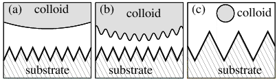
The lateral quantum electrodynamic Casimir force has been measured between a sinusoidally corrugated metal sphere and a corrugated planar wall [54]. An experiment involving a geometrically structured colloid could provide direct access to the lateral critical Casimir force for the geometry (see Figs. 21(b) and 16). Such setups can play a role for moving ratchet-like parts in nano-machines. Using a smooth colloid which is small compared with the corrugation, one may, for example, measure the individual local contributions to normal and lateral critical Casimir force [Fig. 21(c)].
Acknowledgment
The authors thank an anonymous referee for raising the issue of lateral critical Casimir forces decaying algebraically as a function of the lateral coordinate.
Appendix A Undulation of the order parameter contour lines
The behavior of the undulation of the contour lines of the order parameter profile close to a single corrugated substrate (see Subsec. II.3.2) is studied within MFT and a distant wall approximation scheme by introducing a superposition approximation for the order parameter [Eqs. (13) and (14)].
A.1 Distant behavior of the order parameter profile for
Within MFT the order parameter profile at criticality solves the differential equation [Eq. (11)]
| (51) |
Far from the substrate, i.e., for , the order parameter profile contribution due to the corrugation and the underlying planar wall contribution [Eq. (13)] are related as
| (52) |
Thus, for the cubic power of one can neglect quadratic or higher order terms of . Within MFT the underlying effective planar wall contribution [Eqs. (6) and (8)] is
| (53) |
where is the universal surface amplitude for the planar wall system [Eq. (8)] with within MFT [15]. Together with Eq. (14) (i.e., the product ansatz ) and the fact that the underlying effective planar wall contribution is a solution of the corresponding Euler-Lagrange equation Eq. (11), Eq. (51) turns into
| (54) |
Equation (54) holds for and independently and therefore both sides of Eq. (54) are equal to the same constant so that for the part of Eq. (54) depending on one has
| (55) |
A solution of Eq. (55), which is compatible with the periodic boundary conditions of the corrugated system [Fig. 1], is
| (56) |
where with a natural number; is a positive amplitude. We assume that far from the substrate only the main contribution due to the corrugation is significant, i.e., and . For the -dependent part of Eq. (54) one has
| (57) |
Far from the substrate (i.e., ) the underlying effective planar wall contribution Eq. (53) fulfils
| (58) |
Thus, together with from above, Eq. (57) can be written as
| (59) |
with the physically relevant solution
| (60) |
and as a positive amplitude. Accordingly, at criticality the contribution of the corrugation to the order parameter decays exponentially into the bulk, in contrast to the total order parameter, which decays algebraically. Upon inserting the effective planar wall solution, the final approximative expression for the order parameter reads
| (61) |
where . depends only on the corrugation height () and on the wedge angle because for the product depends only on , , and [Eq. (2)].
From Eq. (61) we calculate the undulation of the contour lines, which has been defined in Subsec. II.3.2 as the difference of the maximum and the minimum value of of a given contour line of the order parameter. The positions of the maximum and the minimum and of a contour line correspond to the same values as the crest of an edge or the apex of a wedge of the periodic array of wedges and ridges, i.e., or . Thus, for any contour line far from the substrate one finds
| (62) |
and
| (63) |
Along a contour line the order parameter value is constant which allows one to equate the right-hand sides of Eqs. (62) and (63):
| (64) |
Far from the wall , and quadratic and higher order terms of can be neglected. With the additional assumption that is not much larger than , one can approximate and Eq. (64) becomes
| (65) |
Thus, the undulation of the contour lines of the order parameter decays exponentially into the bulk with the decay constant
| (66) |
A.2 Distant behavior of the order parameter profile for
The order parameter profile for is characterized by the scaling function [Eq. (1)] which we abbreviate as . The procedure follows the one of Subappendix A.1 for . The MFT Euler-Lagrange equation for the scaling function reads
| (67) |
According to Eq. (13) one separates into an effective planar wall contribution and a corrugation contribution:
| (68) |
where is the effective planar wall MFT solution (see Eqs. (5– 8) and Fig. 8):
| (69) |
which corresponds to the bulk value . Far from the substrate , so that one can neglect terms of quadratic or higher order in . Using the product ansatz according to Eq. (14) (i.e., ), upon inserting Eq. (68) into Eq. (67) one finds the following differential equations:
| (70) |
and
| (71) |
Similar to Subappendix A.1 the solution of Eq. (70) is
| (72) |
where and with a natural number . By keeping only the main contribution , Eq. (71) becomes
| (73) |
where is replaced by its bulk value zero because for large distances . Equation (73) is solved by
| (74) |
where is a positive constant. Finally, for the approximate solution for reads
| (75) |
with given by Eq. (69). For one has
| (76) |
Similar to Subappendix A.1 one can directly identify the minimum and the maximum of the contour lines with and . Using the abbreviation
| (77) |
the comparison of the order parameter at these two positions yields
| (78) |
where is a prefactor, which is independent of and includes all possible other prefactors. Far from the substrate , and one can neglect terms of quadratic or higher order of it. With the additional assumptions that is not much larger than unity and is not much smaller than (i.e., is not much larger than ) Eq. (78) simplifies and one finds
| (79) |
where the proportionality constant depends on and . Thus, for the undulation decays exponentially into the bulk with the decay constant
| (80) |
A.3 Distant behavior of the order parameter for
For one has to consider the scaling function [Eq. (1)] abbreviated as . It obeys the differential equation [Eq. (11)]
| (81) |
Following an analogous procedure as in Subappendices A.1 and A.2 and using the ansatz [Eqs. (13) and (14)] one finds
| (82) |
The part of Eq. (82) depending on is solved by
| (83) |
where and . Accordingly, the part of Eq. (82) depending on reads
| (84) |
Far from the wall one can replace by :
| (85) |
With this replacement Eq. (82) is the same as Eq. (73) for , with replacing . Thus, with Eq. (4) the undulation for can be approximated by
| (86) |
where
| (87) |
Appendix B Distant behavior of the lateral critical Casimir force for
In this appendix we discuss the distant wall behavior of the lateral critical Casimir force between two identically structured substrates (see Subsec. III.3) by using a superposition approximation based on Eqs. (13) and (14) and Appendix A.
In Subappendix A.1 the corrugation contribution to the order parameter for close to a single corrugated wall [Fig. 1] has been approximated for large distances from the wall as [Eq. (61)]
| (88) |
where is a positive number which only depends on as and .
For the geometry [Fig. 16] one has to deal with the corrugations of both walls located at and as well as with the lateral shift along the direction. The corrugation contribution of the lower and upper wall in Fig. 16 to the order parameter is [Eq. (88)] and , respectively. The underlying planar wall contribution for the geometry is the order parameter profile between two planar walls at distance in the strong adsorption limit for identical chemical boundary conditions [10]; does not depend on the lateral position variable . In order to determine the distant wall behavior it is convenient to approximate the total order parameter at in the geometry as
| (89) |
The lateral critical Casimir force is given by the integral over the stress tensor component (see Eqs. (34) and (36)):
| (90) |
where is an arbitrary but fixed position in between the two substrates. For simplicity we choose , i.e., the center position in between the two substrates, where the planar wall contribution to the order parameter takes its minimal value, i.e.,
| (91) |
With this the integrand in Eq. (90) reduces to a product of the derivatives of the sum of the corrugation contributions. Performing the integration in Eq. (90) leads to Eq. (47) with the dimensionless amplitude
| (92) |
where within MFT. Note that and is inversely proportional to ; accordingly, is positive and depends only on .
Appendix C Comparison of the lateral critical Casimir force with lateral van der Waals forces
C.1 Lateral van der Waals forces for geometrically structured confinements within the approximation of summing pair potentials
Van der Waals or dispersion forces provide a nonsingular background contribution which adds to the critical Casimir forces. For example, the particles constituting the confining substrates in the geometry [Fig. 16] do not only interact with the fluid, but also among each other, such that their inhomogeneous distribution gives rise to a lateral force acting on the substrates even in the absence of the fluid in between them. The strength of these background forces can be determined by analyzing the confining system without a fluid.
In order to estimate the contribution of the background interaction between the substrate molecules to the total force, we assume their corresponding pair potential to be given by the well known non-retarded van der Waals potential,
| (93) |
where and are the three-dimensional position vectors of the two interacting molecules, the amplitude characterizing the strength of the interaction between the molecules is chosen such that it turns into the Hamaker constant, and and are the number densities of the particles in the two interacting bodies (here because we consider identical substrate materials).
We use the pairwise summation approximation (PWS) in order to calculate the total van der Waals interaction potential between two macroscopic bodies,
| (94) |
where and denote the volumes of the two interacting substrates. Note that for the geometries under consideration, the typical sizes of which are large on molecular scales, assuming a non-retarded van der Waals potential as well as the PWS amount to a severe approximation. But here using them is appropriate because we want to obtain a simple comparison between the strengths of the lateral van der Waals force and the lateral critical Casimir force for the geometry [Fig. 16].
The van der Waals interaction potential per area within the plane corresponding to the lateral van der Waals force for the geometry is given by
| (95) |
where is the value as a function of of the lower substrate surface in Fig. 16,
| (96) |
and is the corresponding value of the upper substrate surface. For identical but shifted corrugations one has , where is the lateral shift between the two substrates along the direction [Fig. 16]. In Eq. (95) only the volumina of the corrugations on top of the two planar substrates have been considered. is the interaction potential between two planar semi-infinite substrates at distance ; it depends only on and therefore does not give rise to a lateral force. With , the integral in Eq. (95) reduces to
| (97) |
The lateral van der Waals force per area corresponds to the derivative of with respect to the lateral shift ,
| (98) |
where . Rescaling the lengths in the integrals in Eq. (98) with the projected width ,
| (99) |
and defining the dimensionless function (corresponding to Eq. (96) and with [Fig. 1]) as
| (100) |
the lateral van der Waals force [Eq. (98)] reads
| (101) |
where plays the role of a dimensionless scaling function of the lateral van der Waals force for the geometry:
| (102) |
with .
C.2 Numerical comparison
In order to gauge the strength of the lateral critical Casimir force [Subsec. III.3], we compare its amplitude with the one of the lateral van der Waals background force obtained within the PWS approximation [Subappendix C.1] for a specifically chosen geometry.
For the amplitude of the lateral critical Casimir force for the geometry we consider at the specific configuration and (i.e., ) [Fig. 16]. For this choice the corresponding lateral critical Casimir force scaling function amplitude has approximately the value (see the solid curve with square symbols in Fig. 18(b))
| (103) |
The corresponding maximum of the lateral critical Casimir force is (see Eq. (45))
| (104) |
The lateral critical Casimir force is given in units of the characteristic thermal energy and the dimensional cross-sectional area within the plane. Accordingly, the maximum of the lateral critical Casimir force per area at criticality for the configuration chosen above is given by
| (105) |
Although the scaling function was determined within mean field theory, its form gives a reasonable approximation for dimensions , too, if one replaces all quantities depending on the dimension of the system by their corresponding value for the actual dimension . In order to obtain an estimate of the strength of the lateral critical Casimir force in we use [24]. As typical length and temperature scales we use nm (i.e., nm, nm, and nm for the specific geometry under consideration) and we take K. With these values, the maximum of the lateral critical Casimir force [Eq. (105)] is of the order of fNm.
In order to estimate the strength of the contribution of the background forces to the total force we use the PWS approximation result for the lateral dispersion force for the geometry [Subappendix C.1]. For the lateral van der Waals force scaling function for the geometry defined above (, , i.e., ) one has [Eq. (102)]
| (106) |
Typical values of the Hamaker constant are of the order of . Using nm as above, we find for the maximum of the lateral van der Waals force [Eq. (101)] for the geometry a typical value of fNm. This means that the background van der Waals interaction calculated within the PWS approximation, which represents the background interaction, is of the order of to of the lateral critical Casimir force. Thus, near criticality the lateral critical Casimir forces are expected to be much stronger than the background forces.
References
- [1] M. E. Fisher and P. G. De Gennes, C. R. Acad. Sci., Paris, Ser. B 287, 207 (1978).
- [2] K. Binder, in Phase Transitions and Critical Phenomena, edited by C. Domb and J. L. Lebowitz (Academic, London, 1983), Vol. 8, p. 1.
- [3] H. W. Diehl, in Phase Transitions and Critical Phenomena, edited by C. Domb and J. L. Lebowitz (Academic, London, 1986), Vol. 10, p. 75.
- [4] A. J. Bray and M. A. Moore, J. Phys. A 10, 1927 (1977).
- [5] T. W. Burkhardt and H. W. Diehl, Phys. Rev. B 50, 3894 (1994).
- [6] M. Krech and S. Dietrich, Phys. Rev. Lett. 66, 345 (1991).
- [7] M. Krech and S. Dietrich, Phys. Rev. A 46, 1886 (1992).
- [8] M. Krech and S. Dietrich, Phys. Rev. A 46, 1922 (1992).
- [9] M. Krech, The Casimir Effect in Critical Systems (World Scientific, Singapore, 1994); and references therein.
- [10] M. Krech, Phys. Rev. E 56, 1642 (1997).
- [11] H. G. B. Casimir, Proc. K. Ned. Akad. Wet. 51, 793 (1948).
- [12] F. Capasso, J. N. Munday, D. Iannuzzi, and H. B. Chan, IEEE J. Quantum Electron. 13, 400 (2007).
- [13] B. M. Law, Prog. Surf. Sci. 66, 159 (2001).
- [14] A. J. Liu and M. E. Fisher, Phys. Rev. A 40, 7202 (1989).
- [15] G. Flöter and S. Dietrich, Z. Phys. B 97, 213 (1995).
- [16] M. D. Brown, B. M. Law, L. Marchand, L. B. Lurio, I. Kuzmenko, T. Gog, and W. A. Hamilton, Phys. Rev. E 75, 061606 (2007a).
- [17] M. D. Brown, B. M. Law, S. Satija, W. A. Hamilton, E. Watkins, J. H. J. Cho, and J. Majewski, J. Chem. Phys. 126, 204704 (2007b).
- [18] R. Garcia and M. H. W. Chan, Phys. Rev. Lett. 88, 086101 (2002).
- [19] M. Fukuto, Y. F. Yano, and P. S. Pershan, Phys. Rev. Lett. 94, 135702 (2005).
- [20] A. Ganshin, S. Scheidemantel, R. Garcia, and M. H. W. Chan, Phys. Rev. Lett. 97, 075301 (2006).
- [21] S. Rafai, D. Bonn, and J. Meunier, Physica A 386, 31 (2007).
- [22] C. Hertlein, L. Helden, A. Gambassi, S. Dietrich, and C. Bechinger, Nature 451, 172 (2008).
- [23] A. Hucht, Phys. Rev. Lett. 99, 185301 (2007).
- [24] O. Vasilyev, A. Gambassi, A. Maciołek, and S. Dietrich, Europhys. Lett. 80, 60009 (2007).
- [25] T. W. Burkhardt and E. Eisenriegler, Phys. Rev. Lett. 74, 3189 (1995); 78, 2867 (1997).
- [26] E. Eisenriegler and U. Ritschel, Phys. Rev. B 51, 13717 (1995).
- [27] A. Hanke, F. Schlesener, E. Eisenriegler, and S. Dietrich, Phys. Rev. Lett. 81, 1885 (1998).
- [28] F. Schlesener, A. Hanke, and S. Dietrich, J. Stat. Phys. 110, 981 (2003).
- [29] E. Eisenriegler, J. Chem. Phys. 121, 3299 (2004).
- [30] S. Kondrat, L. Harnau, and S. Dietrich, J. Chem. Phys. 126, 174902 (2007).
- [31] Y. N. Xia and G. M. Whitesides, Annu. Rev. Mater. Sci. 28, 153 (1998).
- [32] J. Wang, D. K. Thompson, and J. G. Simmons, J. Electrochem. Soc. 145, 2931 (1998).
- [33] D. W. L. Tolfree, Rep. Prog. Phys. 61, 313 (1998).
- [34] Z. Nie and E. Kumacheva, Nature Mater. 7, 277 (2008).
- [35] T. Thorsen, S. J. Maerkl, and S. R. Quake, Science 298, 580 (2002).
- [36] M. Sprenger, F. Schlesener, and S. Dietrich, Phys. Rev. E 71, 056125 (2005).
- [37] M. Sprenger, F. Schlesener, and S. Dietrich, J. Chem. Phys. 124, 134703 (2006).
- [38] A. B. D. Cassie and S. Baxter, Trans. Faraday Soc. 40, 546 (1944).
- [39] M. Tasinkevych and S. Dietrich, Phys. Rev. Lett. 97, 106102 (2006).
- [40] M. Tasinkevych and S. Dietrich, Eur. Phys. J. E 23, 117 (2007).
- [41] L. Harnau, F. Penna, and S. Dietrich, Phys. Rev. E 70, 021505 (2004).
- [42] L. Harnau and S. Dietrich, Europhys. Lett. 73, 28 (2006).
- [43] L. Harnau and S. Dietrich, in Soft Matter, edited by G. Gomper and M. Schick (Wiley-VCH, Weinheim, 2007), Vol. 3, p. 159.
- [44] F. Karimi Pour Haddadan and S. Dietrich, Phys. Rev. E 73, 051708 (2006).
- [45] K. Zhao and T. G. Mason, Phys. Rev. Lett. 99, 268301 (2007).
- [46] A. Hanke, M. Krech, F. Schlesener, and S. Dietrich, Phys. Rev. E 60, 5163 (1999).
- [47] G. Palágyi and S. Dietrich, Phys. Rev. E 70, 046114 (2004).
- [48] J. L. Cardy, J. Phys. A 16, 3617 (1983).
- [49] P. J. van Zwol, G. Palasantzas, and J. Th. M. De Hosson, Phys. Rev. B 77, 075412 (2008).
- [50] T. Emig, A. Hanke, R. Golestanian, and M. Kardar, Phys. Rev. Lett. 87, 260402 (2001).
- [51] T. Emig, A. Hanke, R. Golestanian, and M. Kardar, Phys. Rev. A 67, 022114 (2003).
- [52] H. B. Chan, Y. Bao, J. Zou, R. A. Cirelli, F. Klemens, W. M. Mansfield, and C. S. Pai, Phys. Rev. Lett. 101, 030401 (2008).
- [53] A. Lambrecht and V. N. Marachevsky, e-print arXiv:0806.3142v1 [quant-ph].
- [54] F. Chen, U. Mohideen, G. L. Klimchitskaya, and V. M. Mostepanenko, Phys. Rev. Lett. 88, 101801 (2002).
- [55] R. Büscher and T. Emig, Phys. Rev. Lett. 94, 133901 (2005).
- [56] R. B. Rodrigues, P. A. Maia Neto, A. Lambrecht, and S. Reynaud, Phys. Rev. Lett. 96, 100402 (2006).
- [57] D. A. R. Dalvit, P. A. Maia Neto, A. Lambrecht, and S. Reynaud, J. Phys. A 41, 164028 (2008).
- [58] A. Ashourvan, M. Miri, and R. Golestanian, Phys. Rev. Lett. 98, 140801 (2007).
- [59] T. Emig, Phys. Rev. Lett. 98, 160801 (2007).
- [60] M. Miri and R. Golestanian, Appl. Phys. Lett. 92, 113103 (2008).
- [61] R. B. Rodrigues, P. A. Maia Neto, A. Lambrecht, and S. Reynaud, J. Phys. A 41, 164019 (2008).
- [62] E. Gülari, A. F. Collings, R. L. Schmidt, and C. J. Pings, J. Chem. Phys. 56, 6169 (1972).
- [63] H. W. Diehl and M. Smock, Phys. Rev. B 47, 5841 (1993); 48, 6740 (1993).
- [64] H. B. Tarko and M. E. Fisher, Phys. Rev. Lett. 31, 926 (1973).
- [65] H. B. Tarko and M. E. Fisher, Phys. Rev. B 11, 1217 (1975).
- [66] K. Binder and P. C. Hohenberg, Phys. Rev. B 6, 3461 (1972).
- [67] M. Tröndle, Critical Adsorption and Critical Casimir Forces for Geometrically Structured Confinements (Master Thesis, Universität Stuttgart, 2007).
- [68] W. A. Steele, Surf. Sci. 36, 317 (1973).
- [69] W. E. Carlos and M. W. Cole, Surf. Sci. 91, 339 (1980).
- [70] C. Harrison, C. M. Stafford, W. Zhang, and A. Karim, Appl. Phys. Lett. 85, 4016 (2004).
- [71] J. Genzer and J. Groenewold, Soft Matter 2, 310 (2006).
- [72] M. Schoen and S. H. L. Klapp, in Reviews in Computational Chemistry, edited by K. B. Lipkowitz and T. R. Cundari (Wiley, Hoboken, 2007), Vol. 24, p. 1.
- [73] J. C. Collins, Phys. Rev. D 14, 1965 (1976).
- [74] L. S. Brown, Annals of Physics 126, 135 (1980).
- [75] E. Eisenriegler and M. Stapper, Phys. Rev. B 50, 10009 (1994).
- [76] B. Derjaguin, Kolloid Z. 69, 155 (1934).
- [77] D. Dantchev, F. Schlesener, and S. Dietrich, Phys. Rev. E 76, 011121 (2007).
- [78] D. Dantchev, H. W. Diehl, and D. Grüneberg, Phys. Rev. E 73, 016131 (2006).