Instability of wormholes supported by a ghost scalar field. I. Linear stability analysis
Abstract
We examine the linear stability of static, spherically symmetric wormhole solutions of Einstein’s field equations coupled to a massless ghost scalar field. These solutions are parametrized by the areal radius of their throat and the product of the masses at their asymptotically flat ends. We prove that all these solutions are unstable with respect to linear fluctuations and possess precisely one unstable, exponentially in time growing mode. The associated time scale is shown to be of the order of the wormhole throat divided by the speed of light. The nonlinear evolution is analyzed in a subsequent article.
pacs
04.20.-q, 04.25.-g, 04.40.-bI Introduction
Einstein’s general theory of relativity leads to spectacular predictions like the big bang in the early universe and the existence of black holes and gravitational radiation, all of which are subject to mainstream research in astrophysics and cosmology. More speculative predictions of Einstein’s theory are traversable wormhole geometries [1] consisting of two asymptotically flat ends connected by a common throat through which time-like test particles might travel. Similar constructions can be obtained by removing two holes from a given three-manifold and connecting one with another by a handle, in which case wormholes have been proposed for interstellar travel or building time machines [2, 3].
However, as a consequence of the topological censorship theorem [4] wormholes must be supported by matter fields which are “exotic” in the sense that they violate the averaged null energy condition. In particular, this implies the violation of the weak energy condition which means that some time-like observers measure a negative energy density. On the other hand, it has been shown recently [5] that it is possible to construct wormholes where the violation of the averaged null condition can be made arbitrarily small. Therefore, such wormholes could in principle be supported by quantum fields since quantum effects can lead to violations of the energy conditions.
In this work we assume the existence of stationary wormhole geometries and analyze their stability with respect to small initial perturbations. If stable, the time evolution of such a perturbation may deform the wormhole throat by a small amount, but for large times the perturbation decays to zero and the equilibrium configuration is recovered. If on the other hand the wormhole is unstable, the time evolution may induce large deformations of the throat and in this case it is possible that the wormhole is destroyed making it unsuitable for interstellar travel or building time machines unless the time scale associated to the instability is large enough.
Clearly, the notion of stability depends on the precise matter model that is being considered. In this work, for simplicity, we focus on a massless ghost scalar field. By a ghost field we mean one which violates the dominant energy condition. A massless ghost scalar field consists of a minimally coupled, massless scalar field whose kinetic energy has a reversed sign. Such a field violates the null, and as a consequence also the weak and dominant energy conditions. We analyze the stability of static, spherically symmetric wormhole geometries supported by such fields. We prove in this paper that all such solutions are unstable with respect to linear perturbations and possess precisely one unstable mode which grows exponentially in time. Furthermore, we show that the associated time scale is of the order of the areal radius of the wormhole throat divided by the speed of light. In particular, this means that a wormhole whose throat has an areal radius smaller than , say, decays in a few .
Wormholes supported by scalar fields have been considered before (see, for instance, [6, 7, 8, 9, 10, 11, 12, 13]). In [6, 7, 8] wormholes with a nonminimally coupled scalar field are shown to be unstable with respect to linear fluctuations. In [9] wormholes with a massless, ghost scalar field are constructed. These wormholes are static, spherically symmetric and connect two asymptotic ends which either have both vanishing ADM masses or have ADM masses of opposite signs. Based on a linear stability analysis for the zero mass case it was claimed in [9] that the wormholes with sufficiently small ADM masses are stable. However, a numerical simulation performed in [10] indicates that small perturbations of the zero mass wormholes do not decay under nonlinear evolution and may cause the wormhole to explode or to collapse. Here, we point out that the linear stability analysis of [9] is incomplete in the sense that it only shows stability of the zero mass wormholes for a restricted class of perturbations where the areal radius is unperturbed and the perturbed scalar field vanishes on the throat. However, such perturbations are artificial in some sense because one could imagine perturbing the scalar field by a small ingoing pulse which is supported away from the throat at some time , say. As grows, this pulse travels towards the throat and since the wormhole metric is everywhere regular one expects it to reach and cross the throat at some finite time. On the other hand, requiring that the perturbed scalar field vanishes at the throat corresponds to placing a mirror at the throat which reflects the scalar pulse. As we show in this article, the zero mass wormholes are linearly unstable in the absence of such a mirror, i.e. if one allows perturbations which are not required to vanish at the throat. Furthermore, we generalize the stability analysis to the static, spherically symmetric wormholes with nonvanishing ADM masses and prove that they are linearly unstable as well. In a subsequent paper we analyze the nonlinear evolution of small initial perturbations by numerical means and show that depending on the details of the initial perturbation the wormhole either expands or collapses to a Schwarzschild black hole.
This work is organized as follows. In section II we review the static, spherically symmetric wormhole configurations which are supported by a ghost scalar field. In section III we perform the linear stability analysis. We do so by first generalizing the master equation obtained in [9] to massive wormholes. This master equation turns out to be singular at the throat for both massive and massless wormholes. As a consequence, it requires the solution to decay sufficiently fast as the throat is approached. We then transform the singular master equation in a regular one and show that the new master equation possesses an unstable mode which grows exponentially in time. The associated time scale is computed in section IV by a numerical shooting method. Finally, conclusions are drawn in section V.
II Static, spherically symmetric wormholes supported by a ghost scalar field
We consider a gravitational field which is coupled to a massless ghost scalar field . The action is
where and denote the Ricci scalar and the covariant derivate, respectively, associated to , and with Newton’s constant. Notice that is negative which is the reason for calling the scalar field “ghost”. The corresponding field equations are
| (1) | |||||
| (2) |
where is the Ricci tensor associated to .
For a spherically symmetric field, local coordinates can be chosen such that
| (3) |
where the functions , and , as well as the scalar field depend only on the time coordinate and the spatial coordinate . We are interested in traversable wormhole geometries which consist of a throat connecting two asymptotically flat ends at and , respectively. This means that the areal radius is strictly positive and proportional to for large and that the two-manifold is regular and asymptotically flat at .
For the spherically symmetric ansatz (3) the Einstein equations (1) yield the Hamiltonian constraint , the momentum constraint and the evolution equations and . This and the wave equation (2) yields the evolution equations
| (4) | |||||
| (5) | |||||
| (6) |
and the constraints are
| (7) | |||||
| (8) |
Here, the subscript and refer to the derivatives with respect to and , respectively.
For a static configuration, the scalar field and the metric coefficients , and are independent of . In this case the field equations can be integrated analytically [14, 15]. In order to see this we adopt a gauge where in which case the field equations reduce to
| (9) |
and
| (10) |
The first equation has the general solution with two constants and . By a suitable translation of the coordinate it is always possible to obtain . Furthermore, since we are interested in wormhole geometries with the properties described below equation (3) we need for all . Therefore, we have with some strictly positive constant . The second and third equations in (9) have the solutions
| (11) |
with constants , , , . It follows that
| (12) |
and the metric reads
| (13) |
Notice that the constant rescaling , , , , with a nonvanishing constant leaves the metric unchanged. So for example, we can rescale the coordinates such that in which case and as . Alternatively, we can rescale the coordinates such that in which case and as . With these observations in mind we see that the metric (13) has indeed two asymptotically flat ends at and , respectively. Finally, equation (10) yields the relation
| (14) |
between the parameters and , where we recall that is negative.
Summarizing, we obtain the bi-parametric family of wormhole solutions described by equations (13) and (11,12). This family of solutions has been obtained in [14, 15], and in [9] in the context of wormholes. The solutions can be parametrized by the constants and which are invariant with respect to the rescaling , discussed above. is determined (up to its sign) by the constraint (14). (The sign of is not important since the field equations are invariant with respect to the transformation . Similarly, the parameter has no physical meaning since only the gradient of appears in the equations. Furthermore, it is sufficient to consider nonnegative values for since the solution is invariant with respect to a change of sign of both and .) In order to relate the parameters and to physical quantities we first remark that the areal radius,
has a global minimum at since and . Next, we compute the Misner-Sharp mass function [16]. For the spherically symmetric spacetime metric given by equation (3) it is defined by
For the static solutions described by equations (11,12) this yields
The ADM masses of the two asymptotically flat ends can be computed by considering the asymptotic values of the mass function, which yields and . Notice also that at the throat, .
Therefore, the parameters and determine the ADM masses of the two asymptotic ends, and , and the areal radius of the throat, . Conversely, the areal radius of the throat and the product of the asymptotic masses uniquely determine the parameters and . The particular case yields a zero mass wormhole, , in all other cases the asymptotic masses are nonzero and have opposite signs.
Before concluding this section, we compute the violation of the averaged null energy condition according to [5], which is given by the volume integrals of over the two asymptotically flat ends,
where and are, respectively, the energy density and the radial pressure as measured by static observers. Since for a scalar field and since the Hamiltonian constraint implies that
for static solutions we obtain
| (15) |
We have , so both integrals are strictly negative as expected from the violation of the averaged null energy condition. However, we also see that both integrals can be made arbitrarily small by fixing and letting .
III Linear stability analysis
In this section we analyze the linear stability of the two-parameter family of static wormhole solutions discussed in the previous section. In order to do so, we consider small perturbations of the form
where is the background solution, and where
denotes the variation of . The same applies to the other fields , and . Since there are no dynamical degrees of freedom for a spherical symmetric gravitational field we expect to be able to describe linear fluctuations by a single master equation for the linearized scalar field . In fact this is known [17] to be the case for a large class of matter fields when considering linear fluctuations of static configurations.
However, as we will see in Sec. III.1 the derivation of the master equation for requires a gauge where the areal radius is unperturbed, i.e. where . Since is a scalar field on the two-manifold its linearization transforms as
| (16) |
with respect to infinitesimal coordinate transformations on which are parametrized by the vector field . If it is always possible to achieve the gauge by an appropriate choice of . However, for wormhole topologies, at the throat; hence it is not possible to set everywhere unless we restrict ourselves to perturbations which hold the areal radius of the throat (and any other surface of critical ) fixed.
An alternative approach which does not require the gauge is to replace with the linear combination
| (17) |
which is invariant with respect to infinitesimal coordinate transformations on . In Sec. III.1 we show that the linear perturbations can in fact be described by a master equation which has the form of a wave equation for with potential . However, we will see that this potential diverges as approaches the throat. This property is not entirely surprising since for the gauge-invariant quantity is not well-defined at the throat where diverges.
In Sec. III.2 we transform the singular master equation for into a new master equation which also has the form of a wave equation with a new potential which is everywhere regular, thus facilitating the stability analysis. Furthermore, we prove in Sec. III.3 that the new equation possesses a unique unstable mode which grows exponentially in time. This mode is then shown in III.4 to give rise to an exponentially growing solution of the linearized field equations which is everywhere regular, thus proving the linear instability of the static, spherically symmetric wormholes supported by a massless ghost scalar field.
III.1 Master equation for
Here, we derive the master equation for which is valid for points away from the throat. In order to do so, we first consider the linearized Hamiltonian and momentum constraints which read
| (18) | |||||
| (19) |
With the help of the background equations , and , one can show that these equations possess the first integral
| (20) |
where is a constant whose meaning is explained below.
Now we are ready to obtain the master equation for . For simplicity, we choose a gauge in which that is allowed since we are only considering points away from the throat. In this gauge, and equation (20) reduces to . Equation (21) then yields allowing us to re-express the right-hand side of equation (22) in terms of . The result is the master equation
| (23) |
with the potential
| (24) |
and the forcing term
| (25) |
Since has a gauge-invariant meaning, this equation holds for arbitrary gauges, and not only gauges for which .
For the static wormhole solution (11,12) we have
We see explicitly that the potential diverges at the throat . Therefore, the master equation (23) requires to decay sufficiently fast to zero as in order to be meaningful. If everywhere this in turn requires to be zero at the throat. As an example, the potential for the zero mass wormhole simplifies to and is positive away from the throat11 1 The positivity of led to the claim in [9] that there are no unstable, radial modes.. However, the two asymptotic regions are separated from each other by the infinite potential wall at which acts like a two-sided mirror. Therefore, it follows that with this mirror in place perturbations described by the field cannot grow in time. On the other hand, there is no physical reason for restricting ourselves to perturbations with zero at the throat. In the next subsection we show that equation (23) can be transformed into an equation that is everywhere regular and that does not require to be zero at the throat.
Before we proceed, we analyze the interpretation of the integration constant . For this we notice that the linearization of the static expressions (11,12) with respect to the parameters , and must satisfy the master equation (23) for some value of . Computing the corresponding variation, we find
| (26) |
where . By inserting this expression into equation (23) we find that
| (27) |
Therefore, the integration constant describes static perturbations which change the value of the product of the asymptotic masses, . Since any perturbation can be written as the sum of such a static perturbation plus a perturbation with , we can assume that for the following. The master equation (23) then still admits the static solution
| (28) |
which is obtained from (26) with and . The existence of this solution plays an important role in the next subsection.
III.2 Transformation to a regular equation
Here, we transform the singular master equation (23) into a regular one. For this, and for notational simplicity, we first rescale the coordinates and such that and . Next, we define the two differential operators
where and is the particular solution given in equation (28). Since we can rewrite the master equation (23) as
| (29) |
Applying the operator on both sides of this equation, we find that the quantity satisfies
where
Therefore, satisfies the transformed equation
| (30) |
with the transformed potential . Explicitly, we have
It is not difficult to prove that the function is strictly positive. A short computation gives
| (31) |
Using this, a lengthy calculation yields the following expression for :
| (32) |
where
For the new potential reduces to the simple expression which is strictly negative. For we have
and for . Therefore, is positive for large and negative near the throat . In the next subsection we prove that the new master equation (30) possesses a unique unstable mode of the form
where is the ground state of the Schrödinger operator with negative energy . Notice that decays exponentially to zero as .
III.3 Existence of a bound state with negative energy
Here, we establish the existence of a bound state with negative energy of the Schrödinger operator . For this, we first introduce the new coordinate
which monotonically increases from to and satisfies and . Since is real and bounded, defines a self-adjoint operator on the Hilbert space with domain consisting of the dense subspace of functions whose zeroth, first and second order derivatives are square-integrable on . Let us assume first that . In this case the function
| (33) |
is an eigenfunction of with zero eigenvalue since and since grows linearly in for large . Additionally, this zero mode has precisely one zero, namely at the throat . It follows from the nodal theorem22 2 See, for instance Ref. [18]. that possesses exactly one bound state with negative energy . Its value will be computed in the next section via a numerical shooting method.
For the function is not an eigenfunction of anymore because it does not decay to zero as . Nevertheless, we may still expect the existence of a unique bound state with negative energy by continuity. In order to obtain an upper bound for the ground state energy for the case where , we use the Rayleigh-Ritz33 3 See, for instance Ref. [18]. variational principle,
| (34) |
where denotes the scalar product of . Testing with the particular functions , , gives
where the integral
satisfies the recursion relation
Therefore, we obtain the bound
| (35) |
The function is negative for and positive for . Its minimum lies near for which . Since the minimum of is we obtain the estimate for the ground state energy. This estimate is used as a starting point for a numerical shooting method described in Sec. IV.
III.4 Existence of an exponentially growing mode
To prove that the unstable mode found in the previous subsection gives rise to an exponentially growing regular solution of the linearized field equations we still need to show that there exist perturbation amplitudes , , and which satisfy the linearized field equations, are everywhere regular and grow exponentially in time. Here, we show that such a solution exists indeed.
In order to do so we first notice that satisfies the master equation (23). Next, we choose the infinitesimal coordinates such that . This is possible because for all . In this gauge, , and so we obtain
| (36) |
which is regular everywhere and decays exponentially fast to zero as . We may obtain and from this using the perturbation equations (20) and (22) which, in the gauge yield
A careful calculation using the fact that satisfies and the identity
| (37) |
yields
| (38) | |||||
| (39) |
where is an arbitrary constant which depends on only and could be eliminated by an infinitesimal coordinate transformation. It can be checked that the expressions (36,38,39) also satisfy the evolution equations (21) and the linearization of equation (4) with .
Therefore, we obtain an exponentially growing solution of the linearized field equations which is everywhere regular and decays exponentially to zero for . This proves the linear instability of static, spherically symmetric wormholes supported by a massless ghost scalar field. Their nonlinear evolution are studied in a subsequent paper.
IV Time scale of the instability
In this section we compute the ground state energy of the Schrödinger operator via a numerical shooting method. For this, we first multiply the differential equation on both sides by the factor and obtain
| (40) |
where , and
For the potential is strictly negative. For it is convenient to rewrite the potential as
where and where we have used the identity (37). Since the second term inside the curly brackets is a perfect square we see from this representation that is positive for all values of small enough such that
| (41) |
Therefore, for small , which means that cannot have a local maximum (minimum) if (). For large , on the other hand, decays like and so the normalizable solutions behave like
| (42) |
for large , where .
Our shooting procedure consists in integrating the differential equation (40) starting with the asymptotic solution (42) at some large value of and integrating numerically towards small values of . The integration is stopped as soon as the inequality (41) is satisfied and . If this is the case, the solution must diverge as since cannot have a local maxima in the region where the inequality (41) is satisfied. Therefore, we look for the value of for which as .
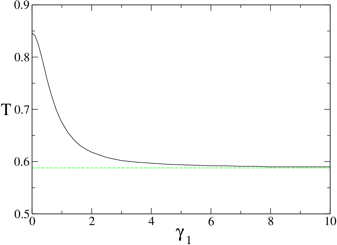
For the numerical integration we compactify the domain by means of the transformation which maps onto and use a fourth order Runge-Kutta integrator with fixed step size. We start with the massless case where the estimates in the previous section provide the bound for the parameter . For the final value for at small is negative, for it is positive. The optimal value for is obtained by bisecting the interval . Then, we increment the value of by a small amount and repeat the above shooting method, finding the optimal value for for the new value of . Continuing this way we obtain the results summarized in table 1 and figure 1, where we show the associated time scale in terms of proper time at the throat of the background solution, , and units of the areal radius of the throat, . This time scale is given by
As is apparent from the results in table 1 and figure 1, the time scale converges to a value of for large values of . The limit is analyzed next.
IV.1 The large limit
In order to understand the behavior of the time scale for large we first notice that the inequality (41) is satisfied for . Therefore, the potential is strictly positive for all and the solution grows at least exponentially fast with increasing on this interval. Since as , the solution must vanish for each fixed as if it is required to have a fixed, finite value at . For this reason, we first replace the coordinate by in the following, and then take the limit .
In terms of the new coordinate the differential equation (40) is transformed into , where , and
where and . From the above, if . Now let be fixed. In the limit we have
and
Therefore, the differential equation (40) converges pointwise to
| (43) |
The operator on the left-hand side is a formally self-adjoint operator on the Hilbert space which is singular at . We obtain a zero mode of this operator by multiplying equation (33) by and taking the limit . This yields
| (44) |
Indeed, it can be checked that (44) solves the differential equation (43) with . Furthermore, this solution decays like for large and as it decays rapidly to zero. Since it has exactly one zero, it follows again from the nodal theorem the existence of a unique bound state with negative energy . A numerical shooting procedure similar to the one described above which starts at some large value of , where , , yields . Since on the other hand in the limit this matches well the asymptotic value obtained in table 1.
V Conclusions
In this article we analyzed the stability of static, spherically symmetric general relativistic wormhole solutions sourced by a massless ghost scalar field. We found that all these solutions are unstable with respect to linear fluctuations of the metric and the scalar field. Furthermore we showed that the time scale associated to this instability is of the order of the areal radius of the throat divided by the speed of light, which is of the order of a few microseconds for a throat of radius of the order of kilometers. Therefore, the instability we found is likely to introduce a rapid growth or collapse of the throat which eventually may destroy the wormhole. In a subsequent paper [19] we follow the nonlinear evolution of the unstable mode by numerical means and show that the wormhole either expands rapidly or collapses to a Schwarzschild black hole.
Our conclusion about the instability of the zero mass wormhole is different from the results presented in Ref. [9]. As explained in Sec. III.1 this is due to the fact that the results in [9] only apply to a restricted class of perturbations which are required to vanish at the throat. As shown in this article, both the massless and massive wormholes are linearly unstable for the more general class of spherically symmetric perturbations which do not necessarily vanish at the throat.
The question arises whether or not there exist wormhole solutions different from the ones considered in this article which are linearly stable. Among the potential options are: i) wormholes with a single asymptotic end obtained by removing two holes from and connecting them to each other by a handle, ii) rotating wormholes, iii) wormholes which are supported by a different kind of matter field, iv) wormholes in modified or higher-dimensional theories of gravity. Regarding option i), it is conceivable that a change in topology affects our instability result. Indeed, since the linear stability of a given solution is directly related to the spectral properties of the linear operator appearing in the perturbation equation it depends on the global structure of the wormhole, and not only on local properties of the throat. Concerning option ii), the possibility that the rotation could stabilize a wormhole has been explored in [12] where an exact solution describing the inner region of a rotating wormhole is constructed. However, based on our instability results, our expectation is that the centrifugal force due to rotation only shifts the equilibrium between the attractive gravitational force and the repulsive force of the ghost scalar field, but does not change its stability. At least we expected that by continuity, slowly rotating wormholes are unstable. Regarding options iii) and iv) there is already a vast amount of results in the literature. To mention only a few examples, it has been shown that static spherically symmetric wormholes in scalar-tensor theories of gravity are linearly unstable [7, 8]. On the other hand, a class of wormhole solutions which are supported by phantom energy have recently been constructed in [20, 21] and shown to be stable with respect to perturbations inside this class [22].
Acknowledgements.
It is a pleasure to thank Ulises Nucamendi and Thomas Zannias for many stimulating discussions. This work was supported in part by grants CIC 4.9, 4.19 and 4.23 to Universidad Michoacana, PROMEP UMICH-PTC-121, UMICH-PTC-195, UMICH-PTC-210 and UMICH-CA-22 from SEP Mexico and CONACyT grant numbers 61173, 79601 and 79995.References
- [1] M.S. Morris and K.S. Thorne. Wormholes in spacetime and their use for interstellar travel: A tool for teaching general relativity. Am. J. Phys., 56:395–412, 1988.
- [2] M.S. Morris, K.S. Thorne, and U. Yurtsever. Wormholes, time machines, and the weak energy condition. Phys. Rev. Lett., 61:1446–1449, 1988.
- [3] V.P. Frolov and I.D. Novikov. Physical effects in wormholes and time machines. Phys. Rev. D, 42:1057–1065, 1990.
- [4] J.L. Friedman, K. Schleich, and D.M. Witt. Topological censorship. Phys. Rev. Lett., 71:1486–1489, 1993.
- [5] M. Visser, S. Kar, and N. Dadhich. Traversable wormholes with arbitrarily small energy condition violations. Phys. Rev. Lett., 90:201102, 2003.
- [6] K.A. Bronnikov and S. Grinyok. Instability of wormholes with a nonminimally coupled scalar field. Grav. Cosmol., 7:297–300, 2001.
- [7] K.A. Bronnikov and S.V. Grinyok. Conformal continuations and wormhole instability in scalar-tensor gravity. Grav. Cosmol., 10:237–, 2004.
- [8] K.A. Bronnikov and A.A. Starobinsky. No realistic wormholes from ghost-free scalar-tensor phantom dark energy. JETP Lett., 85:1–5, 2007.
- [9] C. Armendáriz-Picón. On a class of stable, traversable Lorentzian wormholes in classical general relativity. Phys. Rev. D, 65:104010, 2002.
- [10] Hisa aki Shinkai and Sean A. Hayward. Fate of the first traversible wormhole: Black hole collapse or inflationary expansion. Phys. Rev. D, 66:044005, 2002.
- [11] S.V. Sushkov and S-W. Kim. Cosmological evolution of a ghost scalar field. Gen. Rel. Grav., 36:1671–1678, 2004.
- [12] T. Matos and D. Nuñez. Rotating scalar field wormhole. Class. Quant. Grav., 23:4485–4496, 2006.
- [13] J. Estevez Delgado and T. Zannias. On wormholes and black holes solutions of Einstein gravity coupled to a K-massless scalar field. J. Phys. Conf. Ser., 66:012029, 2007.
- [14] H.G. Ellis. Ether flow through a drainhole: A particle model in general relativity. J. Math. Phys., 14:104–118, 1973.
- [15] K.A. Bronnikov. Scalar-tensor theory and scalar charge. Acta Phys. Polonica B, 4:251–266, 1973.
- [16] C.W. Misner and D.H. Sharp. Relativistic equations for adiabatic, spherically symmetric gravitational collapse. Phys. Rev., 136:B571–B576, 1964.
- [17] O. Brodbeck, M. Heusler, and N. Straumann. Pulsations of spherically symmetric systems in general relativity. Phys. Rev. D, 53:765–761, 1996.
- [18] R. Courant and D. Hilbert. Methods of Mathematical Physics, Volume I. Wiley Classics Edition, 1989.
- [19] J. A. González, F. S. Guzmán, and O. Sarbach. Instability of wormholes supported by a ghost scalar field II: Nonlinear evolution. http://arxiv.org/abs/0806.13708, to appear in Class. Quantum Grav.
- [20] S.V. Sushkov. Wormholes supported by a phantom energy. Phys. Rev. D, 71:043520, 2005.
- [21] F.S.N. Lobo. Phantom energy traversable wormholes. Phys. Rev. D, 71:084011, 2005.
- [22] F.S.N. Lobo. Stability of phantom wormholes. Phys. Rev. D, 71:124022, 2005.