Sampling Spatially Correlated Clutter

The ${\mathcal{G}}_{A}^{0}(\alpha,\gamma,n)$ distribution is characterized by the following probability density function:

being $n\geq 1$ the number of looks of the image, which is controlled at the image generation process, and $\mathbb{I}_{T}(\cdot)$ the indicator function of the set $T$. The parameter $\alpha$ describes the roughness, being small values (say $\alpha\leq-15$) usually associated to homogeneous targets, like pasture, values ranging in the $(-15,-5]$ interval usually observed in heterogeneous clutter, like forests, and big values ($-5<\alpha<0$ for instance) commonly seen when extremely heterogeneous areas are imaged. The parameter $\gamma$ is related to the scale, in the sense that if $Z$ is ${\mathcal{G}}_{A}^{0}(\alpha,1,n)$ distributed then $Z_{A}=\sqrt{\gamma}Z$ obeys a ${\mathcal{G}}_{A}^{0}(\alpha,\gamma,n)$ law.

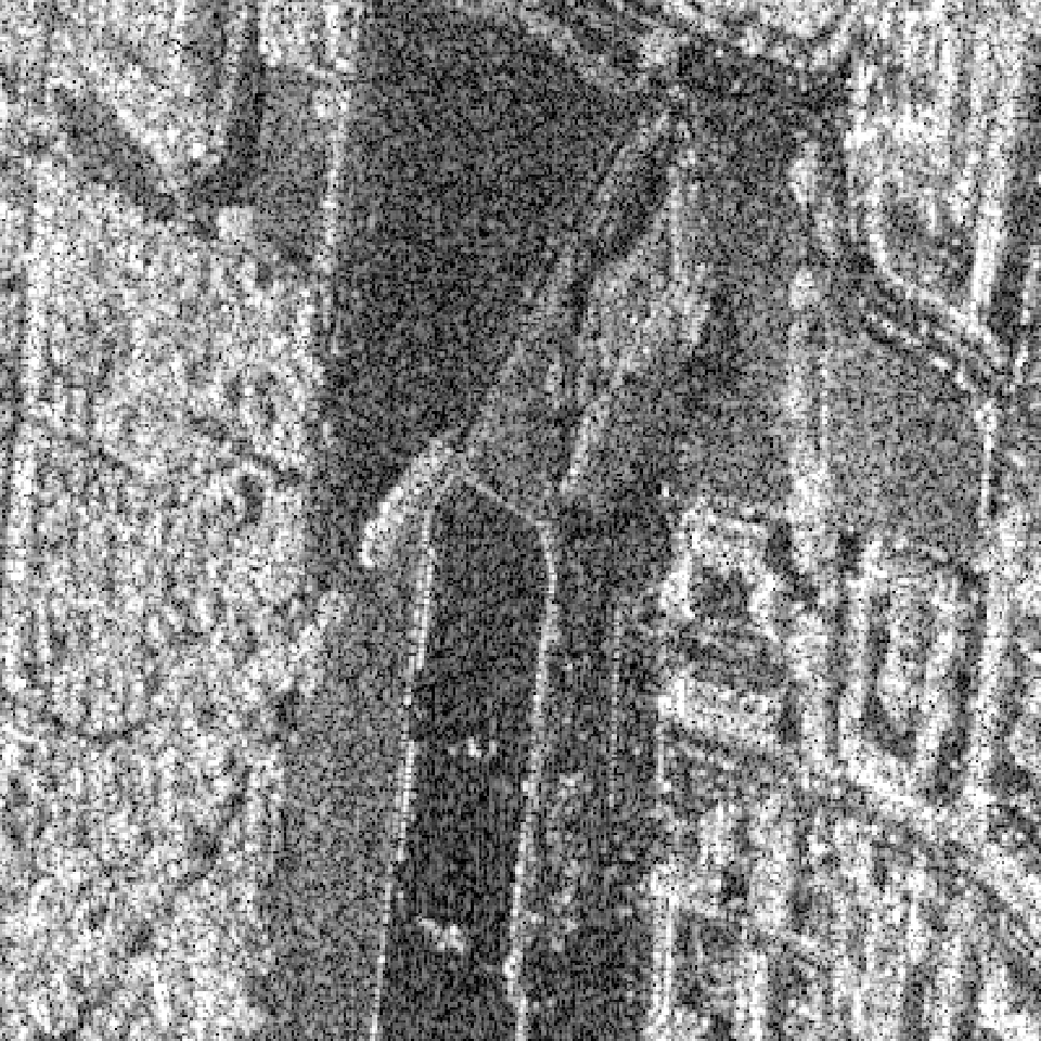
A SAR image over a suburban area of München, Germany, is shown in Figure 1. It was obtained with E-SAR, an experimental polarimetric airborne sensor operated by the German Aerospace Agency (Deutsches Zentrum für Luft- und Raumfahrt – DLR e. V.) The data here shown were generated in single look format, and exhibit the three discussed types of roughness: homogeneous (the dark areas to the middle of the image), heterogeneous (the clear area to the left) and extremely heterogeneous (the clear area to the right).

The $r$-th moments of the ${\mathcal{G}}_{A}^{0}(\alpha,\gamma,n)$ distribution are

when $-r/2\leq\alpha<0$ the $r$-th order moment is infinite. Using equation (2) the mean and variance of a ${\mathcal{G}}_{A}^{0}(\alpha,\gamma,n)$ distributed random variable can be computed:

Figure 2 shows three densities of the ${\mathcal{G}}_{A}^{0}(\alpha,\gamma,n)$ distribution for the single look ($n=1$) case. These densities are normalized so that the expected value is $1$ for every value of the roughness parameter. This is obtained using equation (2) for setting the scale parameter $\gamma=\gamma_{\alpha,n}=n\left(\Gamma(-a)\Gamma(n)/\left(\Gamma(-a-1/2)\Gamma(n+1/2)\right)\right)^{2}$. These densities illustrate the three typical situations described above: homogeneous areas ($\alpha=-15$, dashes), heterogeneous clutter ($\alpha=-5$, dots) and an extremely heterogeneous target ($\alpha=-1.5$, solid line).

Following Barndorff-Nielsen and Blæsild [6], it is interesting to see these densities as log probability functions, particularly because the ${\mathcal{G}}_{A}^{0}$ is closely related to the class of Hyperbolic distributions [7]. Figure 3 shows the densities of the ${\mathcal{G}}_{A}^{0}(-3,1,1)$ and ${\mathcal{N}}(3\pi/16,1/2-9\pi^{2}/256)$ distributions in semilogarithmic scale, along with their mean value $\mu=3\pi/16$. The parameters were chosen so that these distributions have equal mean and variance. The different decays of their tails is evident: the former behaves logarithmically, while the latter decays quadratically. This behavior ensures the ability of the ${\mathcal{G}}_{A}^{0}$ distribution to model data with extreme variability.

Besides being essential for the simulation technique here proposed, cumulative distribution functions are needed for carrying out goodness of fit tests and for the proposal of estimators based on order statistics. It can be seen in [3, 8, 9] that the cumulative distribution function of a ${\mathcal{G}}_{A}^{0}(\alpha,\gamma,n)$ distributed random variable is given, for every $z>0$, by $G(z,(\alpha,\gamma,n))=\Upsilon_{2n,-2\alpha}(-\alpha z^{2}/\gamma)$, where $\Upsilon_{s,t}$ is the cumulative distribution function of a Snedecor’s $F_{s,t}$ distributed random variable with $s$ and $t$ degrees of freedom. Both $\Upsilon_{\cdot,\cdot}$ and $\Upsilon^{-1}_{\cdot,\cdot}$ are readily available in most platforms for computational statistics.

The single look case is of particular interest since it describes the noisiest images and it exhibits nice analytical properties. The distribution is characterized by the density $f(z;\alpha,\gamma,1)=-\frac{2\alpha}{\gamma^{\alpha}}\,z(\gamma+z^{2})^{\alpha-1}\mathbb{I}_{(0,\infty)}(z)$, whith $-\alpha,\gamma>0$. Its cumulative distribution function is given by $F(t)=1-\left(1+t^{2}/\gamma\right)^{\alpha}\mathbb{I}_{(0,\infty)}(t)$, and its inverse, useful for the generation of random deviates and the computation of quantiles, is given by $F^{-1}(t)=\left(\gamma\left((1-t)^{1/\alpha}-1\right)\right)^{1/2}\mathbb{I}_{(0,1)}(t)$.

Instead of defining the model over $\mathbb{Z}^{2}$, in this section a realistic description of finite-sized fields is made. Let $Z_{A}=(Z_{A}(k,\ell))_{0\leq k\leq N-1,0\leq\ell\leq N-1}$ be the stochastic model that describes the return amplitude image.

The scale property of the parameter $\gamma$ implies that correlation function $\rho_{Z_{A}}$ and $\gamma$ are unrelated and, therefore, it is enough to generate a $Z_{A}^{1}\sim({\mathcal{G}}_{A}^{0}(\alpha,1,n),\rho_{Z_{A}})$ field and then simply multiply every outcome by $\gamma^{1/2}$ to get the desired field.

This paper presents a variation of a method used for simulation of correlated Gamma variables, called Transformation Method, that can be found in [10]. This method can be summarized in the following three steps:

1. 1.

   Generate independent outcomes from a convenient distribution.

2. 2.

   Introduce correlation in these data.

3. 3.

   Transform the correlated observations into data with the desired marginal properties [11].

The transformation that guarantees the validity of this procedure is obtained from the cumulative distribution functions of the data obtained in step 2, and from the desired set of distributions.

Recall that if $U$ is a continuous random variable with cumulative distribution function $F_{U}$ then $F_{U}(U)$ obeys a uniform ${\mathcal{U}}(0,1)$ law and, reciprocally, if $V$ obeys a ${\mathcal{U}}(0,1)$ distribution then $F_{U}^{-1}(V)$ is $F_{U}$ distributed. In order to use this method it is necessary to know the correlation that the random variables will have after the transformation, besides the function $F_{U}^{-1}$.

The method here studied consists of the following steps:

1. 1.

   propose a correlation structure for the ${\mathcal{G}}_{A}^{0}$ field, say, the function $\rho_{Z_{A}}$;

2. 2.

   generate a field of independent identically distributed standard Gaussian observations;

3. 3.

   compute $\tau$, the correlation structure to be imposed to the Gaussian field from $\rho_{Z_{A}}$, and impair it using the Fourier transform without altering the marginal properties;

4. 4.

   transform the correlated Gaussian field into a field of observations of identically distributed ${\mathcal{U}}(0,1)$ random variables, using the cumulative distribution function of the Gaussian distribution ($\Phi$);

5. 5.

   transform the uniform observations into ${\mathcal{G}}_{A}^{0}$ outcomes, using the inverse of the cumulative distribution function of the ${\mathcal{G}}_{A}^{0}$ distribution ($G^{-1}$).

The function that relates $\rho_{Z_{A}}$ and $\tau$ is computed using numerical tools. In principle, there are no restrictions on the possible roughness parameters values that can be obtained by this method, but issues related to machine precision must be taken into account. Another important issue is that not every desired final correlation structure $\rho_{Z_{A}}$ is mapped onto a feasible intermediate correlation structure $\tau$. The procedure is presented in detail in the next section.

The function $\varrho_{(\alpha,n)}$ has the following properties:

1. 1.

   The set $\{\varrho_{(\alpha,n)}(\tau)\colon\tau\in(-1,1)\}$ is strictly included in $(-1,1)$, and depends on the values of $\alpha$.

2. 2.

   The function $\varrho_{(\alpha,n)}$ is strictly increasing in $(-1,1)$.

3. 3.

   The values $\varrho_{(\alpha,n)}(\tau)$ are strictly negative for all $\tau<0$.

Let $\eth_{(\alpha,n)}$ be the inverse function of $\varrho_{(\alpha,n)}$. Then, in order to calculate its value for a fixed $\rho\in(-1,1)$, we have to solve the following equation in $\tau$:

Then, it follows from the properties of $\varrho_{(\alpha,n)}$, that for certain values of $\alpha$ the set of $\tau$ such that this equation is solvable is a strict subset of $(-1,1)$. Table 1 shows some values of the function $\eth_{(\alpha,n)}$ for specific values of $\rho$, $n$ and $\alpha$. Figure 4 shows $\tau$ as a function of $\rho$ for the $n=1$ case and varying values of $\alpha$, and it can be seen that the smaller $\alpha$ the closer this function is to the identity. This is sensible, since the ${\mathcal{G}}_{A}^{0}$ distribution becomes more and more symmetric as $\alpha\to-\infty$ and, therefore, simulating outcomes from this distribution becomes closer and closer to the problem of obtaining Gaussian deviates.

Figure 5 presents the same function for $\alpha=-1.5$ and varying number of looks. It is noticeable that $\tau$ is far less sensitive to $n$ than to $\alpha$, a feature that suggests a shortcut for computing the values of Table 1: disregarding the dependence on $n$, i.e., considering $\tau(\rho,\alpha,n)\simeq\tau(\rho,\alpha,n_{0})$ for a fixed convenient $n_{0}$.

The source FORTRAN file with routines for computing the functions $\varrho_{(\alpha,n)}$ and $\eth_{(\alpha,n)}$ can be obtained from the first author of this paper.

The process $\zeta$, that consists of spatially correlated standard Gaussian random variables, will be generated using a spectral technique that employs the Fourier transform. This method has computational advantages with respect to the direct application of a convolution filter. Again, the concern here is to define a finite process instead of working on $\mathbb{Z}^{2}$ for the sake of simplicity.

Consider the following sets:

Let $\rho\colon R_{1}\longrightarrow(-1,1)$ be a function, extended onto $\overline{R_{N}}$ by:

Let $Z_{A}=(Z_{A}(k,\ell))_{0\leq k\leq N-1,0\leq l\leq N-1}$ be a ${\mathcal{G}}_{A}^{0}(\alpha,\gamma,n)$ stochastic process with correlation function $\rho_{Z_{A}}$ defined by

Assume that $\tau(k,\ell)=\eth_{(\alpha,n)}(\rho(k,\ell))$ is defined for all $(k,\ell)$ in $R_{N}$.

Let ${\mathcal{F}}(\tau)\colon R_{N}\longrightarrow\mathbb{C}$ be the normalized Fourier Transform of $\tau$, that is,

Let $\psi\colon R_{N}\longrightarrow\mathbb{C}$ be defined by $\psi(k,\ell)=\sqrt{{\mathcal{F}}(\tau)(k,\ell)}$ and let the function $\theta:\overline{R_{N}}=\{(k,\ell)\colon-(N-1)\leq k,\ell\leq N-1\}\longrightarrow\mathbb{R}$ be defined by

(the normalized inverse Fourier Transform of $\psi$) for all $(k,\ell)\in{R_{N}}$; and

A straightforward calculation shows that

for all $(k,\ell)\in R_{N}$.

Finally we define $\zeta=(\zeta(i,j))_{0\leq i\leq N-1,0\leq j\leq N-1}$ by

where $\xi=(\xi(k,\ell))_{(k,\ell).\in R_{N}}$ is a Gaussian white noise with standard deviation $1$.

Then it is easy to prove that $\zeta=(\zeta(i,j))_{0\leq i\leq N-1,0\leq j\leq N-1}$ is a stochastic process such that $\zeta(i,j)$ is a standard Gaussian random variable with correlation function $\tau_{\zeta}$ satisfying (3).

The results presented in previous sections were implemented using the IDL Version 5.3 Win 32 [14] development platform, with the following algorithm:

References

• [1] A. C. Frery, H.-J. Müller, C. C. F. Yanasse, and S. J. S. Sant’Anna. A model for extremely heterogeneous clutter. IEEE Transactions on Geoscience and Remote Sensing, 35(3):648–659, May 1997.
• [2] A. C. Frery, A. H. Correia, C. D. Rennó, C. C. Freitas, J. Jacobo-Berlles, M. E. Mejail, and K. L. P. Vasconcellos. Models for synthetic aperture radar image analysis. Resenhas (IME-USP), 4(1):45–77, 1999.
• [3] M. E. Mejail, A. C. Frery, J. Jacobo-Berlles, and O. H. Bustos. Approximation of distributions for SAR images: proposal, evaluation and practical consequences. Latin American Applied Research, 31:83–92, 2001.
• [4] O. H. Bustos, M. M. Lucini, and A. C. Frery. M-estimators of roughness and scale for GA0-modelled SAR imagery. EURASIP Journal on Applied Signal Processing, 2002(1):105–114, Jan. 2002.
• [5] F. Cribari-Neto, A. C. Frery, and M. F. Silva. Improved estimation of clutter properties in speckled imagery. Computational Statistics and Data Analysis, 40(4):801–824, 2002.
• [6] O. E. Barndorff-Nielsen and P. Blæsild. Hyperbolic distributions and ramifications: Contributions to theory and applications. In C. Taillie and B. A. Baldessari, editors, Statistical distributions in scientific work, pages 19–44. Reidel, Dordrecht, 1981.
• [7] A. C. Frery, C. C. F. Yanasse, and S. J. S. Sant’Anna. Alternative distributions for the multiplicative model in SAR images. In International Geoscience and Remote Sensing Symposium: Quantitative Remote Rensing for Science and Applications, pages 169–171, Florence, Jul. 1995. IEEE Computer Society. IGARSS’95 Proc.
• [8] M. E. Mejail, J. C. Jacobo-Berlles, A. C. Frery, and O. H. Bustos. Classification of SAR images using a general and tractable multiplicative model. International Journal of Remote Sensing. In press.
• [9] M. E. Mejail, J. Jacobo-Berlles, A. C. Frery, and O. H. Bustos. Parametric roughness estimation in amplitude SAR images under the multiplicative model. Revista de Teledetección, 13:37–49, 2000.
• [10] O. H. Bustos, A. G. Flesia, and A. C. Frery. Generalized method for sampling spatially correlated heterogeneous speckled imagery. EURASIP Journal on Applied Signal Processing, 2001(2):89–99, June 2001.
• [11] C. Oliver and S. Quegan. Understanding Synthetic Aperture Radar Images. Artech House, Boston, 1998.
• [12] A. K. Jain. Fundamentals of Digital Image Processing. Prentice-Hall International Editions, Englewood Cliffs, NJ, 1989.
• [13] S. M. Kay. Modern Spectral Estimation: Theory & Application. Prentice Hall, Englewood Cliffs, NJ, USA, 1988.
• [14] Research Systems. Using IDL. http://www.rsinc.com, 1999.
Appendix A Estimating correlation structure with Pearson’s method
Consider the image 𝐳\mathbf{z} with MM rows and NN columns
𝐳=[z⁡(0,0)⋯z⁡(N−1,0)⋮⋱⋮z⁡(0,M−1)⋯z⁡(N−1,M−1)]\mathbf{z}=\left[\begin{array}[c]{ccc}z(0,0)&\cdots&z(N-1,0)\\ \vdots&\ddots&\vdots\\ z(0,M-1)&\cdots&z(N-1,M-1)\end{array}\right]
and nvn_{v} a positive integer smaller than min⁡(M,N)\min(M,N). Define nc=[N/(2​nv)]n_{c}=\left[N/(2n_{v})\right] and nf=[M/(2​nv)]n_{f}=\left[M/(2n_{v})\right], where [x]=max⁡{k∈ℕ:k≤x}\left[x\right]=\max\left\{k\in\mathbb{N}\colon k\leq x\right\} for every real number xx. For each i=0,…,nc−1i=0,\ldots,n_{c}-1 and each j=0,…,nf−1j=0,\ldots,n_{f}-1 define 𝐜⁡(i,j)\mathbf{c}(i,j) the submatrix of 𝐳\mathbf{z} of size 2​nv×2​nv2n_{v}\times 2n_{v} given by
𝐜⁡(i,j)=[z⁡(2​nv​i,2​nv​j)⋯z⁡(2​nv​i+2​nv−1,2​nv​j)⋮⋱⋮z⁡(2​nv​i,2​nv​j+2​nv−1)⋯z⁡(2​nv​i+2​nv−1,2​nv​j+2​nv−1)],\mathbf{c}(i,j)=\left[\begin{array}[c]{ccc}z(2n_{v}i,2n_{v}j)&\cdots&z(2n_{v}i+2n_{v}-1,2n_{v}j)\\ \vdots&\ddots&\vdots\\ z(2n_{v}i,2n_{v}j+2n_{v}-1)&\cdots&z(2n_{v}i+2n_{v}-1,2n_{v}j+2n_{v}-1)\end{array}\right],
and let 𝐳v​(i,j)\mathbf{z}_{v}(i,j) be the submatrix of 𝐜⁡(i,j)\mathbf{c}(i,j) of size nv×nvn_{v}\times n_{v} given by
𝐳v​(i,j)=[z⁡(2​nv​i,2​nv​j)⋯z⁡(2​nv​i+nv−1,2​nv​j)⋮⋱⋮z⁡(2​nv​i,2​nv​j+nv−1)⋯z⁡(2​nv​i+nv−1,2​nv​j+nv−1)].\mathbf{z}_{v}(i,j)=\left[\begin{array}[c]{ccc}z(2n_{v}i,2n_{v}j)&\cdots&z(2n_{v}i+n_{v}-1,2n_{v}j)\\ \vdots&\ddots&\vdots\\ z(2n_{v}i,2n_{v}j+n_{v}-1)&\cdots&z(2n_{v}i+n_{v}-1,2n_{v}j+n_{v}-1)\end{array}\right].
We will consider that 𝐳v​(i,j)\mathbf{z}_{v}(i,j), for every i=0,…,nc−1i=0,\ldots,n_{c}-1 and every j=0,…,nf−1j=0,\ldots,n_{f}-1 is a sample of the random matrix
𝐙=[Z⁡(0,0)⋯Z⁡(nv−1,0)⋮⋱⋮Z⁡(0,nv−1)⋯Z⁡(nv−1,nv−1)].\mathbf{Z}=\left[\begin{array}[c]{ccc}Z(0,0)&\cdots&Z(n_{v}-1,0)\\ \vdots&\ddots&\vdots\\ Z(0,n_{v}-1)&\cdots&Z(n_{v}-1,n_{v}-1)\end{array}\right].
The autocorrelation function of the random matrix 𝐙\mathbf{Z} is defined as
ρ𝐙​((m,n),(k,ℓ))=E⁡(Z⁡(m,n)​Z​(k,ℓ))−μZ​(m,n)​μZ​(k,ℓ)σZ​(m,n)​σZ​(k,ℓ),\rho_{\mathbf{Z}}((m,n),(k,\ell))=\frac{E(Z(m,n)Z(k,\ell))-\mu_{Z}(m,n)\mu_{Z}(k,\ell)}{\sigma_{Z}(m,n)\sigma_{Z}(k,\ell)},
where μZ​(k,ℓ)=E⁡(Z⁡(k,ℓ))\mu_{Z}(k,\ell)=E(Z(k,\ell)) and σZ​(k,ℓ)=V​a​r​(Z⁡(k,ℓ))\sigma_{Z}(k,\ell)=\sqrt{Var(Z(k,\ell))}, for every 0≤m,n,k,ℓ≤nv−10\leq m,n,k,\ell\leq n_{v}-1.
The function ρ𝐙\rho_{\mathbf{Z}} can be estimated using Pearson’s sample correlation coefficient based on 𝐳v​(i,j)\mathbf{z}_{v}(i,j), i=0,…,nc−1i=0,\ldots,n_{c}-1 and j=0,…,nf−1j=0,\ldots,n_{f}-1, i.e., for 0≤m,n,k,ℓ≤nv−10\leq m,n,k,\ell\leq n_{v}-1 by
r𝐙​((m,n),(k,ℓ))=C𝐙​((m,n),(k,ℓ))s𝐙​(m,n)​s𝐙​(k,ℓ),r_{\mathbf{Z}}((m,n),(k,\ell))=\frac{C_{\mathbf{Z}}((m,n),(k,\ell))}{s_{\mathbf{Z}}(m,n)s_{\mathbf{Z}}(k,\ell)},
where
C𝐙​((m,n),(k,ℓ))\displaystyle C_{\mathbf{Z}}((m,n),(k,\ell)) =∑j=0nf−1∑i=0nc−1(z⁡(2​nv​i+m,2​nv​j+n)−z¯​(m,n))​(z⁡(2​nv​i+k,2​nv​j+ℓ)−z¯​(k,ℓ)),\displaystyle=\sum\limits_{j=0}^{n_{f}-1}\sum\limits_{i=0}^{n_{c}-1}\left(z(2n_{v}i+m,2n_{v}j+n)-\overline{z}(m,n)\right)\left(z(2n_{v}i+k,2n_{v}j+\ell)-\overline{z}(k,\mathbf{\ell})\right),
s𝐙​(m,n)\displaystyle s_{\mathbf{Z}}(m,n) =∑j=0nf−1∑i=0nc−1(z⁡(2​nv​i+m,2​nv​j+n)−z¯​(m,n))2,\displaystyle=\sqrt{\sum\limits_{j=0}^{n_{f}-1}\sum\limits_{i=0}^{n_{c}-1}\left(z(2n_{v}i+m,2n_{v}j+n)-\overline{z}(m,n)\right)^{2}},
z¯​(m,n)\displaystyle\overline{z}(m,n) =1nc​nf​∑j=0nf−1∑i=0nc−1z⁡(2​nv​i+m,2​nv​j+n).\displaystyle=\frac{1}{n_{c}n_{f}}\sum\limits_{j=0}^{n_{f}-1}\sum\limits_{i=0}^{n_{c}-1}z(2n_{v}i+m,2n_{v}j+n).