Matrix Models, Gauge Theory and Emergent Geometry

It has been shown in [26, 27, 28, 29] that the differential calculus on the fuzzy sphere is three dimensional and as a consequence, treating gauge fields as one-forms, a generic gauge field, $\vec{A}$ has $3$ components. Each component $A_{a}$, $a=1,2,3$, is an element of $Mat_{N}$ and the $U(1)$ gauge symmetry of the commutative sphere will become a $U(N)$ gauge symmetry on the fuzzy sphere with gauge transformations implemented as $A_{a}{\longrightarrow}UA_{a}U^{\dagger}+U[L_{a},U^{\dagger}]$ where $U\in U(N)$. In this approach to gauge fields on the fuzzy sphere, ${\bf S}^{2}_{N}$, it is difficult to split the vector field $\vec{A}$ in a gauge-covariant fashion into a tangent gauge field and a normal scalar field. However, we can write a gauge-covariant expression for the normal scalar field as $\Phi=\frac{1}{2}(x_{a}A_{a}+A_{a}x_{a}+\frac{A_{a}^{2}}{\sqrt{c_{2}}})$. In the commutative limit, $N\rightarrow\infty$, we have $A_{a}\rightarrow{\cal A}_{a}$ and $\Phi\rightarrow\varphi=n_{a}{\cal A}_{a}$ and the splitting into gauge field and scalar field becomes trivial being implemented by simply writing ${\cal A}_{a}=n_{a}{\varphi}+a_{a}$, with $n_{a}a_{a}=0$, where $\vec{n}$ is the unit vector on ${\bf S}^{2}$, $\varphi=\vec{n}\cdot\vec{{\cal A}}$ is the normal gauge-invariant component of $\vec{{\cal A}}$ and $\vec{a}$ is the tangent gauge field.

For this formulation of gauge field theory on the fuzzy sphere the most general action (up to quartic power in $A_{a}$) on ${{\bf S}}^{2}_{N}$ is then

$\displaystyle\framebox{$S_{N}[A]=\frac{1}{4g^{2}N}TrF_{ab}^{2}-\frac{1}{2g^{2}N}{\epsilon}_{abc}Tr\left[\frac{1}{2}F_{ab}A_{c}-\frac{i}{6}[A_{a},A_{b}]A_{c}\right]+\frac{2m^{2}}{g^{2}N}Tr\Phi^{2}+\frac{{\rho}}{g^{2}N}Tr\Phi.$}$

(3.1)

In above $Tr{\bf 1}=N$ and $F_{ab}=i[L_{a},A_{b}]-i[L_{b},A_{a}]+{\epsilon}_{abc}A_{c}+i[A_{a},A_{b}]$ is the covariant curvature, and $S_{N}[0]=0$. The limit $m^{2}{\longrightarrow}\infty$ gives a large mass to the scalar component and effectively projects it out of the spectrum of small fluctuations.

The associated continuum action $S_{\infty}$ is then at most quadratic in the field and as a consequence the theory is largely trivial, consisting of a gauge field and a scalar field that have a mixing in their joint propagator. Indeed we can show that

$\displaystyle S_{\infty}=\frac{1}{4g^{2}}\int\frac{d{\Omega}}{4{\pi}}\bigg[(f_{ab})^{2}-4{\epsilon}_{abc}f_{ab}n_{c}\varphi-2({\cal L}_{a}\varphi)^{2}+4(1+2m^{2}){\varphi}^{2}+4\rho{\varphi}\bigg],$

(3.2)

where $f_{ab}$ is the curvature of the tangent field $a_{a}$ and $f_{ab}=i{\cal L}_{a}a_{b}-i{\cal L}_{b}a_{a}+{\epsilon}_{abc}a_{c}$. As one can immediately see this theory consists of a $2$-component gauge field $a_{a}$ that mixes with a scalar field $\varphi$, i.e. the propagator mixes the two fields. In the following we will primarily be interested in the case with $\rho=0$. We see also that the presence of the scalar field means that the geometry is completely specified, in that all the ingredients of the spectral triple are supplied by this field. In contrast a two dimensional gauge theory on its own would not be sufficient to specify the geometry.

We introduce $\tilde{\alpha}^{4}=\frac{1}{g^{2}}=\beta$ where $\beta$ can be interpreted as an inverse temperature and we can rewrite the above gauge action (3.1) (shifted by constants and dropping the subscript $N$) in terms of $D_{a}=L_{a}+A_{a}$ as follows:

	$\displaystyle S^{(0)}[D]$	$\displaystyle=$	$\displaystyle\frac{1}{4g^{2}N}TrF_{ab}^{2}-\frac{1}{2g^{2}N}{\epsilon}_{abc}Tr\left[\frac{1}{2}F_{ab}A_{c}-\frac{i}{6}[A_{a},A_{b}]A_{c}\right]-\frac{\tilde{\alpha}^{4}c_{2}}{6}$		(3.3)
		$\displaystyle=$	$\displaystyle\frac{\tilde{\alpha}^{4}}{N}\bigg[-\frac{1}{4}Tr[D_{a},D_{b}]^{2}+\frac{2i}{3}{\epsilon}_{abc}TrD_{a}D_{b}D_{c}\bigg].$

	$\displaystyle V[D]$	$\displaystyle=$	$\displaystyle\frac{2m^{2}}{g^{2}N}Tr\Phi^{2}+\frac{{\rho}}{g^{2}N}Tr\Phi-\frac{m^{2}c_{2}}{2g^{2}}+\frac{\rho\sqrt{c_{2}}}{2g^{2}}$		(3.4)
		$\displaystyle=$	$\displaystyle\frac{\tilde{\alpha}^{4}}{N}\bigg[\frac{m^{2}}{2c_{2}}Tr(D_{a}^{2})^{2}+\left(\frac{{\rho}}{2\sqrt{c_{2}}}-m^{2}\right)Tr(D_{a}^{2})\bigg].$

The complete action functional is then:

$\displaystyle\framebox{$S[D]\equiv{S}^{(0)}[D]+V[D]=S_{N}[A]-\frac{\tilde{\alpha}^{4}c_{2}}{6}-\frac{\tilde{\alpha}^{4}m^{2}c_{2}}{2}+\frac{\tilde{\alpha}^{4}\rho\sqrt{c_{2}}}{2},$}$

(3.5)

and the constants are chosen so that $S[0]=0$. The action takes the rather simple form

$$\framebox{$S[D]=\frac{\tilde{\alpha}^{4}}{N}Tr\big[-\frac{1}{4}[D_{a},D_{b}]^{2}+\frac{2i}{3}{\epsilon}_{abc}D_{a}D_{b}D_{c}+\frac{m^{2}}{2c_{2}}(D_{a}^{2})^{2}-\mu D_{a}^{2}\big]$}$$

(3.6)

where $\mu=m^{2}-\frac{{\rho}}{2\sqrt{c_{2}}}$. It is invariant under unitary transformations $U(N)$ and global rotations $SO(3)$. Extrema of the model are given by the reducible representations of $SU(2)$ and commuting matrices. For sufficiently small $\rho$ and with $c_{2}=(N^{2}-1)/4$ the classical absolute minima of the model is given by the irreducible representation of $SU(2)$ of dimension $N$. Small fluctuations around this background can then be seen to have the geometrical content of a Yang-Mills and scalar multiplet on a background fuzzy sphere as described in the previous section. As we will see, for small enough coupling or low temperature, these configurations also give the ground state of the fluctuating system. For very small negative values of the parameter $\mu$, and for $m=0$ there is a local minimum at $D_{a}=0$ and a global minimum at $D_{a}\sim L_{a}$, separated by a barrier. As $\mu$ is made more negative the difference in energy (or Euclidean action) between the two extrema becomes less and eventually for $\mu=-\frac{2}{9}$ the two minima become degenerate, one occurring at $D_{a}=0$ while the other occurs at $D_{a}=\frac{2}{3}L_{a}$ and they are separated by a barrier whose maximum occurs at $D_{a}=\frac{1}{3}L_{a}$.

In this special case (i.e. $m=0$ and $\mu=-\frac{2}{9}$ or equivalently $\rho=\frac{4}{9}\sqrt{c_{2}}$) the action takes the form

$$S[D]=\frac{\tilde{\alpha}^{4}}{N}\bigg(\frac{i}{2}Tr[D_{a},D_{b}]+\frac{1}{3}{\epsilon}_{abc}D_{c}\bigg)^{2}.$$

(3.7)

and we see that the configurations $D_{a}=0$ and $D_{a}=\frac{2}{3}L_{a}$ both give zero action, however there is a unique configuration with $D_{a}=0$ while there is an entire $SU(N)$ manifold of configurations $D_{a}=\frac{2}{3}UL_{a}U^{\dagger}$ which are equivalent. The classical model has a first order transition at $m=0$ for $\mu=-\frac{2}{9}$ and the classical ground state switches from $D_{a}=\phi L_{a}$, where $\phi=(1+\sqrt{1+4\mu})/2$, for $\mu>-2/9$ to $D_{a}=0$ for $\mu<-2/9$. The quantity $\phi$ is therefore a useful order parameter for this transition. However, one would expect fluctuations to have a significant effect on this classical picture.

In fact both theoretical and numerical studies show that in the fluctuating theory, the fuzzy sphere phase only exists for $\mu>-2/9$ [30].

The quantum version of the model is taken to be that obtained by functional integration with respect to the gauge field. This amounts to integration over the three Hermitian matrices $D_{a}$ with Dyson measure and the partition function $Z$ is given by

	$\displaystyle Z=\int dD_{a}e^{-{S}[D]}=e^{-\frac{3N^{2}}{4}\log{{\alpha}^{4}}}\int dX_{a}e^{-N\hat{S}[X]}\penalty\ ,\penalty\ X_{a}=\alpha D_{a}\penalty\ ,\penalty\ \tilde{\alpha}=\alpha\sqrt{N}$
	$\displaystyle\hat{S}[X]=-\frac{1}{4}Tr[X_{a},X_{b}]^{2}+\frac{2i\alpha}{3}{\epsilon}_{abc}TrX_{a}X_{b}X_{c}+\frac{m^{2}}{2c_{2}}Tr(X_{a}^{2})^{2}+\left(\frac{\rho{\alpha}^{2}}{2\sqrt{c_{2}}}-m^{2}\alpha^{2}\right)Tr(X_{a}^{2}).$

The latter form of the expression (in terms of $X_{a}$) allows us to take $\tilde{\alpha}=0$ and we see that this limit is equivalent to removing all but the leading commutator squared term. Also the quartic term proportional to $m^{2}$ survives. However if $m^{2}$ and $\rho$ are scaled appropriately with $\tilde{\alpha}$ only the Chern-Simons term ${\epsilon}_{abc}TrX_{a}X_{b}X_{c}$ is removed.

The set of gauge equivalent configurations is parameterized by the $SU(N)$ group manifold which is compact, so there is no need to gauge fix and the functional integral is well defined, being an ordinary integral over ${\bf R}^{3N^{2}}$. However, the volume of the gauge group diverges in the limit $N\rightarrow\infty$ and to make contact with the commutative formulation it is convenient to gauge fix in the standard way.

In the background field gauge formulation we separate the field as $X_{a}=\tilde{\alpha}D_{a}+Q_{a}$. The action is invariant under $D_{a}{\longrightarrow}D_{a}$, $Q_{a}{\longrightarrow}UQ_{a}U^{\dagger}+U[D_{a},U^{\dagger}]$.

Following the standard Faddeev-Popov procedure [31] and taking the background field configuration to be $D_{a}=\phi L_{a}$ one finds, keeping $m^{2}$ fixed as the $N\rightarrow\infty$ limit is taken, that $F=-\ln Z$ is given by

$\displaystyle\framebox{$\frac{F}{N^{2}}=\frac{3}{4}\log\tilde{\alpha}^{4}+\frac{\tilde{\alpha}^{4}}{2}\bigg[\frac{{\phi}^{4}}{4}-\frac{{\phi}^{3}}{3}+m^{2}\frac{{\phi}^{4}}{4}-\mu\frac{\phi^{2}}{2}\bigg]+\log\tilde{\alpha}{\phi},$}$

(3.9)

with $\mu=m^{2}-\frac{\rho}{2\sqrt{c_{2}}}$.

The most notable feature of this expression is that the entire fluctuation contribution is summarized in the logarithmic term $\log(\tilde{\alpha}\phi)$. From (3.9) we see that the effective potential for the order parameter $\phi$ is

$$\frac{V_{\rm eff}}{2c_{2}}=\tilde{\alpha}^{4}\left[\frac{\phi^{4}}{4}-\frac{\phi^{3}}{3}+m^{2}\frac{\phi^{4}}{4}-\mu\frac{\phi^{2}}{2}\right]+\log\phi^{2}$$

(3.10)

The effective potential is not bounded below at $\phi=0$ due to the $\ln\phi$ term. However, our analysis assumes the existence of a fuzzy sphere ground state and so the effective potential can only be trusted in this phase. It has a local minimum for $\phi$ positive and sufficiently large $\tilde{\alpha}$ and in this regime the fuzzy sphere configuration exists, for lower values of $\tilde{\alpha}$ our numerical study indicates that the model is indeed in a different phase.

Setting $\phi\frac{\partial F}{\partial\phi}=0$ (or equivalently $\phi\frac{\partial V_{\rm eff}(\phi)}{\partial\phi}=0$) gives

$$\frac{\tilde{\alpha}^{4}}{2}\bigg[{\phi}^{4}-{\phi}^{3}+m^{2}{\phi}^{4}-\mu{\phi^{2}}\bigg]+1=0,$$

(3.11)

the solution of which specifies $\phi$. We define the average of the action, which will be one of the principal observables of our numerical study, as

$${\cal S}=<S>/N^{2}=\tilde{\alpha}^{4}\frac{d}{d\tilde{\alpha}^{4}}\bigg(\frac{F}{N^{2}}\bigg).$$

(3.12)

Then a direct computation and use of eq. (3.11) yields

$\displaystyle\framebox{${\cal S}=\frac{3}{4}-\frac{\tilde{\alpha}^{4}{\phi}^{3}}{24}-\frac{\tilde{\alpha}^{4}\mu{\phi}^{2}}{8}.$}$

(3.13)

We can also compute the expected radius of the sphere

$$\frac{1}{R}=\frac{<TrD_{a}^{2}>}{Nc_{2}}=-\frac{2}{\tilde{\alpha}^{4}}\frac{dF}{d\mu}=\phi^{2}$$

(3.14)

This can also be calculated directly in perturbation theory as

$\displaystyle\frac{1}{R}$

$\displaystyle=$

$\displaystyle{\phi}^{2}+\frac{1}{c_{2}\tilde{\alpha}^{4}{\phi}^{2}}Tr_{3}Tr_{N^{2}}(\frac{1}{{\cal L}_{c}^{2}{\delta}_{ab}+4m^{2}x_{a}x_{b}}).$

(3.15)

Hence, we conclude that the expected inverse radius of the fuzzy sphere is given by

$\displaystyle\framebox{$\frac{1}{R}={\phi}^{2}.$}$

(3.16)

Also

$\displaystyle\frac{<Tr((D_{a}^{2})^{2})>}{2N^{3}c_{2}}=\frac{1}{\tilde{\alpha}^{4}}\frac{\partial}{{\partial}m^{2}}\bigg(\frac{F}{N^{2}}\bigg)=\frac{{\phi}^{4}}{8},$

(3.17)

which yields

$\displaystyle\framebox{$\frac{<Tr(D_{a}^{2})^{2}>}{2N^{3}c_{2}}=\frac{\phi^{4}}{8}.$}$

(3.18)

Scaling $(D_{a})_{ij}$ to $(1-\epsilon)(D_{a})_{ij}$ in both the action and measure amounts to a simple coordinate transformation which leaves the partition function invariant. However it also leads to the nontrivial identity

$\displaystyle\frac{\tilde{\alpha}^{4}}{N}<K_{m}>=3N^{2}\penalty\ ,\penalty\ K_{m}=Tr\bigg(-[D_{a},D_{b}]^{2}+2i\epsilon_{abc}D_{a}D_{b}D_{c}-2m^{2}D_{a}^{2}+\frac{2m^{2}}{c_{2}}(D_{a}^{2})^{2}\bigg).$

(3.19)

Using this identity we can express

$\displaystyle{\cal S}=\frac{3}{4}+\frac{\tilde{\alpha}^{4}}{6N^{3}}<i{\epsilon}_{abc}TrD_{a}D_{b}D_{c}>-\frac{\tilde{\alpha}^{4}}{2N^{3}}m^{2}<TrD_{a}^{2}>.$

(3.20)

or equivalently in the form

$\displaystyle{\cal S}=1+\frac{\tilde{\alpha}^{4}}{12N^{3}}<Tr[D_{a},D_{b}]^{2}>-\frac{\tilde{\alpha}^{4}}{3N^{3}}m^{2}<TrD_{a}^{2}>-\frac{\tilde{\alpha}^{4}}{6N^{3}c_{2}}m^{2}<Tr(D_{a}^{2})^{2}>.$

We define the Yang-Mills and Chern-Simons actions by

$\displaystyle\framebox{$4{\rm YM}=-\frac{<Tr[D_{a},D_{b}]^{2}>}{2Nc_{2}},\rm{and}\penalty\ 3{\rm CS}=\frac{<i{\epsilon}_{abc}TrD_{a}D_{b}D_{c}>}{Nc_{2}}.$}$

(3.22)

Then using the above results we find

$\displaystyle 4{\rm YM}={\phi}^{4}+\frac{8}{\tilde{\alpha}^{4}}\penalty\ \rm{and}\penalty\ 3{\rm CS}=-{\phi}^{3}.$

(3.23)

In the above we have extensively used the fact that $\phi$ must satisfy (3.11) and taken $\rho=0$ i.e. $\mu=m^{2}$.

Another significant observable for our numerical study is the specific heat $C_{v}$ defined as

$\displaystyle C_{v}:=\frac{<S^{2}>-<S>^{2}}{N^{2}}=\frac{<S>}{N^{2}}-\tilde{\alpha}^{4}\frac{d}{d\tilde{\alpha}^{4}}\bigg(\frac{<S>}{N^{2}}\bigg).$

(3.24)

A direct calculation yields

$\displaystyle\framebox{$C_{v}=\frac{3}{4}+\frac{\tilde{\alpha}^{5}\phi}{32}(\phi+2m^{2})\frac{d\phi}{d\tilde{\alpha}}.$}$

(3.25)

Finally one can recover perturbation theory in the coupling $g^{2}=1/\tilde{\alpha}^{4}$ by expanding in $1/\tilde{\alpha}^{4}$. In particular the one-loop predictions are obtained by using the solution of (3.11) expanded to first order which is $\tilde{\alpha}{\longrightarrow}\infty$ given by

$\displaystyle\phi=1-\frac{2}{1+2m^{2}}\frac{1}{\tilde{\alpha}^{4}}+O(\frac{1}{\tilde{\alpha}^{8}}).$

(3.26)

In the next section we will look at the solution of (3.11) in more detail and the consequences for the transition.

Let us now examine the predictions for the quantum transition as determined by $F$ given in (3.9) or the effective potential (3.10) which we repeat here for convenience

$\displaystyle\framebox{$\frac{V_{\rm eff}}{2c_{2}}=\tilde{\alpha}^{4}\bigg[\frac{\phi^{4}}{4}-\frac{\phi^{3}}{3}+m^{2}\frac{\phi^{4}}{4}-\mu\frac{\phi^{2}}{2}\bigg]+\log\tilde{\phi}^{2}.$}$

(3.27)

But first let us review the classical case. The only difference between the full quantum potential (3.10) and the corresponding classical potential is the quantum induced logarithm of $\phi$, which as we will see plays a crucial role. The extrema of the classical potential occur at

$$\bar{\phi}=(1+m^{2})\phi=\left\{0,\penalty\ \frac{1-\sqrt{1+4t}}{2},\penalty\ \frac{1+\sqrt{1+4t}}{2}\right\}.$$

(3.28)

where $t=\mu(1+m^{2})$. The first and last expressions are local minima and the middle one is the maximum of the barrier between them. For $\mu$ positive the global minimum is the third expression, i.e. the largest value of $\phi$. When written in terms of $\bar{\phi}$ we see the potential takes the same form as that for $m=0$ and we can read off that if $\mu$ is sent negative then this minimum becomes degenerate with that at $\phi=0$ at $t=\mu(1+m^{2})=-\frac{2}{9}$ and the maximum height of the barrier is given by $\frac{\tilde{\alpha}^{4}}{324(1+m^{2})^{3}}$. When $\mu=m^{2}$ the minimum is clearly $\phi=1$, i.e $D_{a}=L_{a}$ for all $m$ and this is separated from the local minimum at $\phi=0$ by a barrier. The classical transition therefore has the same character as that of the $m=0$ model and the transition is 1st order and occurs only when $\rho$ is tuned to a critical value.

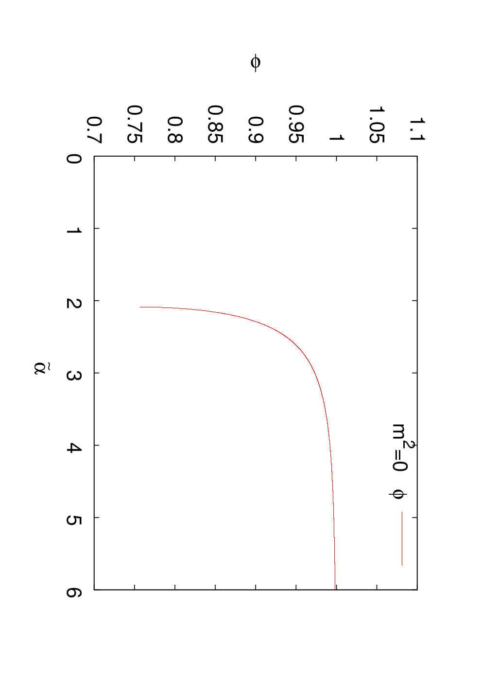
Let us now consider the effect of the fluctuation induced logarithm of $\phi$. The potential is plotted in figure 1 for different values of $\tilde{\alpha}$ and $\mu=m^{2}=20$. The condition $V^{{}^{\prime}}_{\rm eff}(\phi)=0$ gives us extrema of the model. For large enough $\tilde{\alpha}$ (or low enough temperature) and large enough $m$ and $\mu$ it admits four real solutions two for positive $\phi$ and two for negative $\phi$. The largest of the positive $\phi$ solutions can be identified with the least free energy and therefore the ground state of the system in this phase of the theory. It will determine the actual radius of the sphere. The second positive solution is the local maximum (figure 1) of $V_{\rm eff}(\phi)$ and will determine the height of the barrier in the effective potential. As the coupling is decreased (or the temperature increased) these two solutions merge and the barrier disappears. This is the critical point of the model and it has no classical counterpart since, in the classical case, the barrier between the two minima never disappears. For smaller couplings than this critical coupling $\tilde{\alpha}_{*}$ the fuzzy sphere solution $D_{a}={\phi}L_{a}$ no longer exists and the effective potential cannot be relied on. This is in accord with our numerical simulations which indicate that as the matrix size is increased the radius as defined in (3.14) appears to go to zero.

The condition when the barrier disappears is

$\displaystyle V^{{}^{\prime\prime}}_{\rm eff}=\frac{\tilde{\alpha}^{4}}{2}\big[3{\phi}^{2}-2\phi+3m^{2}{\phi}^{2}-\mu\big]-\frac{1}{{\phi}^{2}}=0.$

(3.29)

Solving both (3.11) and (3.29) yields $4(1+m^{2})\phi^{2}_{*}-3\phi_{*}-2\mu=0$ and therefore the critical values

$\displaystyle\framebox{$\bar{\phi}_{*}=\frac{3}{8}(1+\sqrt{1+\frac{32t}{9}}).$}$

(3.30)

$\displaystyle\framebox{$g_{*}^{2}=\frac{1}{\tilde{\alpha}_{*}^{4}}=\frac{{\phi}_{*}^{2}({\phi}_{*}+2\mu)}{8}.$}$

(3.31)

where as defined earlier $\bar{\phi}_{*}=\phi/(1+m^{2})$ and $t=\mu(1+m^{2})$. Setting both $m^{2}=0$ and $\mu=0$ yields

$\displaystyle\framebox{${\phi}_{*}=\frac{3}{4}\penalty\ ,\penalty\ \tilde{\alpha}_{*}^{4}=(\frac{8}{3})^{3}.$}$

(3.32)

while setting $m=0$ alone leads to no significant simplification and we still have $\phi_{*}=\bar{\phi}_{*}$ with $t=\mu$.

If we take $\mu$ negative as in the discussion of the last section we see that $g_{*}$ goes to zero at $t=-1/4$ and the critical coupling $\tilde{\alpha}_{*}$ is sent to infinity and therefore for $t<-\frac{1}{4}$ the model has no fuzzy sphere phase. This case arises when

$$\rho>2\sqrt{c_{2}}(m^{2}+\frac{1}{4(1+m^{2})}).$$

(3.33)

However, in the region $-\frac{1}{4}<\mu<-\frac{2}{9}$ the action (3.6) is completely positive. It is therefore not sufficient to consider only the configuration $D_{a}=\phi L_{a}$, but rather all $SU(2)$ representations must be considered. Furthermore for large $\tilde{\alpha}$ the ground state will be dominated by those representations with the smallest Casimir. This means that there is no fuzzy sphere solution for $\mu<-\frac{2}{9}$. A result that we also observe in simulations and in agreement with the result of [30]. We therefore see that the classical transition described above is significantly affected by fluctuations and in particular the fuzzy sphere phase dissapears when $\rho$ is increased to the special value of $\frac{4\sqrt{c_{2}}}{9}$.

The other limit of interest is the limit $\mu=m^{2}{\longrightarrow}\infty$. In this case

$\displaystyle\framebox{${\phi}_{*}=\frac{1}{\sqrt{2}}\penalty\ ,\penalty\ \tilde{\alpha}^{4}_{*}=\frac{8}{m^{2}}.$}$

(3.34)

This means that the phase transition is located at a smaller value of the coupling constant $\tilde{\alpha}$ as $m$ is increased. In other words the region where the fuzzy sphere is stable is extended to lower values of the coupling or higher temperatures. These results agree nicely with numerical data.

As we cross the critical value of $\tilde{\alpha}$, a rather exotic phase transition occurs where the geometry disappears as the temperature is increased. The fuzzy sphere phase has the background geometry of a two dimensional spherical non-commutative manifold which macroscopically becomes a standard commutative sphere for $N\rightarrow\infty$. The fluctuations are then of a $U(1)$ gauge theory which mixes with a scalar field on this background. In the high temperature phase, which we call a matrix phase, the order parameter $\phi$ is not well defined and the fluctuations are around diagonal matrices so the model is a pure matrix one corresponding to a zero dimensional Yang-Mills theory in the large $N$ limit. The fuzzy sphere phase occurs for $\tilde{\alpha}>\tilde{\alpha}_{*}$ while the matrix phase occurs for $\tilde{\alpha}<\tilde{\alpha}_{*}$.

Since $\phi=0$ is not a solution of equation (3.11) the extremal equation can be rearranged and when expressed in terms of $\bar{\phi}$ takes the form

$\displaystyle P(\bar{\phi})\equiv\bar{\phi}^{4}-\bar{\phi}^{3}-t\bar{\phi}^{2}+\frac{2}{a^{4}}=0.$

(3.35)

where $a^{4}=\tilde{\alpha}^{4}/(1+m^{2})^{3}$. By the substitution $\bar{\phi}=(1-4x)\tilde{\phi}+x$, $P(\bar{\phi})$ can be brought to the form of a

$\displaystyle\tilde{\phi}^{4}-\tilde{\phi}^{3}-\lambda\tilde{\phi}+\frac{2}{{\tilde{\beta}^{4}}}=0.$

(3.36)

The new parameters $\lambda$ and $\tilde{\beta}$ are given by

	$\displaystyle\lambda=\frac{x}{(1-4x)^{3}}\big[x+\frac{4t}{3}\big]\penalty\ ,$		(3.37)
	$\displaystyle\frac{2}{\tilde{\beta}^{4}}=\frac{1}{(1-4x)^{4}}\bigg[\frac{2(1+m^{2})^{3}}{\tilde{\alpha}^{4}}-\frac{1}{4}\bigg(x+\frac{m^{2}(1+m^{2})}{3}\bigg)\bigg(x+\frac{5m^{2}(1+m^{2})}{3}\bigg)\bigg]\penalty\ ,$		(3.38)

and the shift $x$ must take one of the two values

$\displaystyle x\longrightarrow x_{\pm}=\frac{1}{4}(1\pm\sqrt{1+\frac{8t}{3}}).$

(3.39)

We choose $x=x_{-}$ since $x_{-}(0)=0$ and so this case allows us to easily recover the case with $\mu=m^{2}=0$ and for $m^{2}{\longrightarrow}0$ we get

$\displaystyle x_{-}=-\frac{m^{2}}{3}+O(m^{4})\penalty\ ,\penalty\ \lambda=O(m^{4})\penalty\ ,\penalty\ \frac{2}{\tilde{\beta}^{4}}=\frac{2}{\tilde{\alpha}^{4}}(1-\frac{7}{3}m^{2}+O(m^{4}))$

(3.40)

The two positive solutions of (3.35), $\bar{\phi}_{\pm}$, for general values of $m^{2}$ and $\mu$ are then given by

	$\displaystyle(1+m^{2}){\phi}_{\pm}=\frac{1}{4}\bigg[1+(1-4x)\sqrt{1+{\delta}}{\pm}(1-4x)\sqrt{2-{\delta}+\frac{2}{\sqrt{1+{\delta}}}(1+8\lambda)}\bigg]$
	$\displaystyle{\delta}=4W^{\frac{1}{3}}\bigg[\bigg(1+\sqrt{1-V}\bigg)^{\frac{1}{3}}+\bigg(1-\sqrt{1-V}\bigg)^{\frac{1}{3}}\bigg]$
	$\displaystyle V=\frac{1}{W^{2}}\bigg(\frac{8}{3\tilde{\beta}^{4}}-\frac{\lambda}{3}\bigg)^{3}\penalty\ ,\penalty\ W=\frac{1}{\tilde{\beta}^{4}}+\frac{{\lambda}^{2}}{2}.$		(3.41)

We rewrite the above solution (3.41) as follows, (collecting definitions here for completeness)

	$\displaystyle t=\mu(m^{2}+1)\penalty\ ,\penalty\ a^{4}=\frac{\tilde{\alpha}^{4}}{(1+m^{2})^{3}}$
	$\displaystyle q=1+\frac{8t}{3}-\frac{a^{4}t^{3}}{27}\penalty\ ,\penalty\ p=q^{2}-\frac{(\frac{8}{3}+\frac{a^{4}t^{2}}{9})^{3}}{a^{4}}.$		(3.42)

Then we can show that

$\displaystyle(1-4x)^{3}(1+8\lambda)=1+4t\penalty\ ,\penalty\ W=\frac{q}{(1+\frac{8t}{3})^{3}a^{4}}\penalty\ ,\penalty\ V=1-\frac{p}{q^{2}}.$

(3.43)

and

$\displaystyle\delta=\frac{4d}{1+\frac{8t}{3}}\penalty\ ,\penalty\ d=a^{-\frac{4}{3}}\bigg(\big(q+\sqrt{p}\big)^{\frac{1}{3}}+\big(q-\sqrt{p}\big)^{\frac{1}{3}}\bigg).$

(3.44)

Substituting one finds the relatively simple form

$\displaystyle\framebox{$\bar{\phi}_{\pm}=(1+m^{2}){\phi}_{\pm}=\frac{1}{4}+\frac{1}{2}\sqrt{\frac{1}{4}+\frac{2t}{3}+d}\pm\frac{1}{2}\sqrt{\frac{1}{2}+\frac{4t}{3}-d+\frac{1+4t}{4\sqrt{\frac{1}{4}+\frac{2t}{3}+d}}}.$}$

(3.45)

For completeness the remaining two solutions of the quartic $P(\bar{\phi})=0$ are given by

$\displaystyle\framebox{$\bar{\phi}^{n}_{\pm}=(1+m^{2}){\phi}^{n}_{\pm}=\frac{1}{4}-\frac{1}{2}\sqrt{\frac{1}{4}+\frac{2t}{3}+d}\pm\frac{1}{2}\sqrt{\frac{1}{2}+\frac{4t}{3}-d-\frac{1+4t}{4\sqrt{\frac{1}{4}+\frac{2t}{3}+d}}}.$}$

(3.46)

At the critical point $a=a_{c}$, $p$ becomes zero and the two solutions $\bar{\phi}_{+}$ and $\bar{\phi}_{-}$ are equal.

References

- [1] A. Connes, Noncommutative Geometry, Academic Press, London,1994.
- [2] L. Bombelli, J. H. Lee, D. Meyer and R. Sorkin, Phys. Rev. Lett. 59 (1987) 521.
- [3] N. Seiberg, “Emergent spacetime,” 23rd Solvay Conference In Physics: The Quantum Structure Of Space And Time Edited by D. Gross, M. Henneaux, A. Sevrin. Hackensack, World Scientific, 2007. arXiv:hep-th/0601234.
- [4] J. Ambjørn, R. Janik, W. Westra and S. Zohren, Phys. Lett. B 641 (2006) 94 [arXiv:gr-qc/0607013].
- [5] T. Azuma, S. Bal, K. Nagao and J. Nishimura, JHEP 0405 (2004) 005 [arXiv:hep-th/0401038].
- [6] P. Castro-Villarreal, R. Delgadillo-Blando and B. Ydri, Nucl. Phys. B 704 (2005) 111 [arXiv:hep-th/0405201].
- [7] D. O’Connor and B. Ydri, JHEP 0611 (2006) 016 [arXiv:hep-lat/0606013].
- [8] B. Ydri, arXiv:hep-th/0110006.
- [9] D. O’Connor, Mod. Phys. Lett. A 18 (2003) 2423.
- [10] A. P. Balachandran, S. Kürkçüoǧlu and S. Vaidya, arXiv:hep-th/0511114.
- [11] H. Grosse, C. Klimčík and P. Prešnajder, Commun. Math. Phys. 180 (1996) 429 [arXiv:hep-th/9602115].
- [12] R. C. Myers, JHEP 9912 (1999) 022 [arXiv:hep-th/9910053].
- [13] A. Y. Alekseev, A. Recknagel and V. Schomerus, JHEP 0005 (2000) 010 [arXiv:hep-th/0003187].
- [14] J. Hoppe, MIT Ph.D. Thesis, (1982). J. Madore, Class. Quantum. Grav. 9 (1992) 69.
- [15] Rodrigo Delgadillo-Blando, Denjoe O’Connor and Badis Ydri, “Geometry in transition: A model of emergent geometry,” Phys. Rev. Lett. 100 (1987) 201601 arXiv:0712.3011 [hep-th].
- [16] H. Steinacker, Nucl. Phys. B 679 (2004) 66 [arXiv:hep-th/0307075].
- [17] T. Azuma, K. Nagao and J. Nishimura, JHEP 0506 (2005) 081 [arXiv:hep-th/0410263].
- [18] H. Steinacker and R. J. Szabo, arXiv:hep-th/0701041.
- [19] D. Dou and B. Ydri, Nucl. Phys. B 771 (2007) 167 [arXiv:hep-th/0701160].
- [20] N. Kawahara, J. Nishimura and S. Takeuchi, JHEP 0705 (2007) 091 [arXiv:0704.3183 [hep-th]].
- [21] H. Steinacker, arXiv:0708.2426 [hep-th].
- [22] P. Di Francesco, P. H. Ginsparg and J. Zinn-Justin, Phys. Rept. 254 (1995) 1 [arXiv:hep-th/9306153].
- [23] V. G. Knizhnik, A. M. Polyakov and A. B. Zamolodchikov, Mod. Phys. Lett. A 3 (1988) 819.
- [24] S. Minwalla, M. Van Raamsdonk and N. Seiberg, JHEP 0002 (2000) 020 [arXiv:hep-th/9912072].
- [25] J. Fröhlich and K. Gawȩdzki, Conformal Field Theory and Geometry of Strings, Lectures given at Mathematical Quantum Theory Conference, Vancouver, Canada, 4-8 Aug 1993. Published in Vancouver 1993, Proceedings, Mathematical quantum theory, Vol. 1 57-97, [arXiv:hep-th/9310187].
- [26] H. Grosse and J. Madore, “A Noncommutative version of the Schwinger model,” Phys. Lett. B 283 (1992) 218.
- [27] U. Carow-Watamura and S. Watamura, “Differential calculus on fuzzy sphere and scalar field,” Int. J. Mod. Phys. A 13 (1998) 3235 [arXiv:q-alg/9710034].
- [28] U. Carow-Watamura and S. Watamura, “Noncommutative geometry and gauge theory on fuzzy sphere,” Commun. Math. Phys. 212 (2000) 395 [arXiv:hep-th/9801195].
- [29] H. Grosse, J. Madore and H. Steinacker, “Field theory on the q-deformed fuzzy sphere. I,” J. Geom. Phys. 38 (2001) 308 [arXiv:hep-th/0005273].
- [30] T. Azuma, S. Bal and J. Nishimura, Phys. Rev. D 72 (2005) 066005 [arXiv:hep-th/0504217].
- [31] L.D. Faddeev and V.N. Popov, Phys.Lett.25B,29 (1967).
- [32] D. E. Berenstein, M. Hanada and S. A. Hartnoll, JHEP 0902 (2009) 010 [arXiv:0805.4658 [hep-th]].
- [33] C. Nash and D. O’Connor, J. Phys. A 42 (2009) 012002 [arXiv:0809.2960 [hep-th]].
- [34] E.H.Lieb, Phys.Rev.Lett.73,2158 (1994).