CHIRAL UNITARY DYNAMICS OF HADRONS AND HADRONS IN A NUCLEAR MEDIUM
Abstract
In this talk I summarize recent findings around the description of axial vector mesons as dynamically generated states from the interaction of pseudoscalar mesons and vector mesons, dedicating some attention to the two states. Then I review the generation of open and hidden charm scalar and axial states, and how some recent experiment supports the existence of the new hidden charm scalar state predicted. I present recent results showing that the low lying baryon resonances for S= can be obtained as bound states or resonances of two mesons and one baryon in coupled channels. Then show the differences with the S= case, where the appears also dynamically generated from the two pion one nucleon system, but the does not appear, indicating a more complex structure of the Roper resonance. Finally I shall show how the state X(2175), recently discovered at BABAR and BES, appears naturally as a resonance of the system.
1 Introduction
The combination of nonperturbative unitary techniques in coupled channels with the QCD information contained in the chiral Lagrangians has allowed one to extend the application domain of traditional Chiral Perturbation theory to a much larger range of energies where many low lying meson and baryon resonances appear. For instance, for the interactions between the members of the lightest octet of pseudoscalars, one starts with the chiral Lagrangian of ref. [1, 2] and selects the set of channels that couple to certain quantum numbers. Then, independently of using either the Bethe-Salpeter equation in coupled channels [3], the N/D method [4] or the Inverse Amplitude Method [5], the well known scalar resonances , , and appear as poles in the obtained L=0 meson-meson partial waves. These resonances are not introduced by hand, they appear naturally as a consequence of the meson interaction and they qualify as ordinary bound states or resonances in coupled channels. These are states that we call dynamically generated, by contrast to other states which would rather qualify as states, such as the [6]. Similarly, in the baryon sector, the interaction of the pseudoscalar mesons with baryons of the octet of the proton generates dynamically resonances [7, 8, 9, 10, 11, 12] and the interaction of the pseudoscalar mesons with baryons of the decuplet of the generates resonances [13, 14]. These last two cases can be unified using SU(6) symmetry as done in [15]. This field has proved quite productive and has been further extended by combining pseudoscalar mesons with vector mesons, which lead to the dynamical generation of axial vector mesons like the , , etc [16, 17]. Also in the charm sector one has obtained in this way scalar mesons with charm, like the [18, 19, 20, 21], axial vector mesons with charm like the [16, 22, 23], or hidden charm scalars like a predicted state and two hidden charm axial states, with opposite C-parity, one of which corresponds to the state. In what follows we briefly discuss these latter cases.
Paralelly with these developments investigation has started regarding systems with three hadrons not studied so far, like two mesons and a baryon, or three mesons. A new formalism is developed, based on the Faddeev equations and the on shell scattering amplitudes of the different components. This can be done because one can prove that there are cancellations between the off shell part of these amplitudes and the three body contact forces that originate from the same chiral lagrangians. This novel finding should stimulate thoughts around conventional Faddeev equations which rely upon the full off shell extrapolation of the amplitudes, and eventually require some three body forces that must be put by hand to reproduce the data. I shall report on several states which are obtained within this new formalism and which can be associated to well known resonances.
2 Axial vector mesons dynamically generated
As shown in detail in [16, 17], starting from a standard chiral Lagrangian for the interaction of pseudoscalar mesons of the octet of the and vector mesons of the octet of the , and unitarizing in coupled channels solving the coupled Bethe-Salpeter equations, one obtains the scattering matrix for pseudoscalar mesons with vectors for different quantum numbers, which contains poles that can be associated to known resonances like the , , etc. The SU(3) decomposition of
| (1) |
leads here to two octets, unlike in the case of the interaction of pseudoscalars among themselves where there is only room for the representation. This is why here one finds different G-parity states like the and , the , , plus an extra that one can identify with the singlet state. One should then find two states, which do not have defined G-parity. One might think that these states are the and the states. However the theory fails to predict a state with such a large mass as the and with its decay properties. Instead, in [17] two states were found with masses close by, given, after some fine tuning, by 1197 MeV and 1284 MeV, and widths of about 240 MeV and 140 MeV, respectively [24]. The interesting thing about these states is that the first one couples most strongly to , while the second state couples most strongly to . One could hope that these two states could be observed experimentally. Indeed, this is the case as was shown in the recent work [24] by looking at two reactions which have either or in the final state and which clearly show the peak at different positions, as one can observe in fig. 1.
 |
 |
 |
 |
 |
 |
It is interesting to recall that in the experimental analysis done in [25] only one resonance was included (together with the which shows up at higher energies), but the background was very large and the peaks appeared from interference of large background terms rather than from the effect of the resonance. Instead in [24], with the introduction of the two resonances obtained in our approach and the background generated by the same chiral unitary approach, together with a contribution from the considered phenomenologically, the description of all data in fig. 1 follows in a natural way.
3 Dynamically generated scalar mesons with open and hidden charm
A generalization to SU(4) of the SU(3) chiral Lagrangian for meson-meson interaction is done in [21] to study meson-meson interaction including charm. The breaking of SU(4) is done as in [26, 27], where the crossed exchange of vector mesons is employed as it accounts phenomenologically for the Weinberg-Tomozawa term in the chiral Lagrangians. With this in mind, when the exchange is due to a heavy vector meson the corresponding term is corrected by the ratio of square masses of the light vector meson to the heavy one (vectors with a charmed quark). We also use a different pattern of SU(4) symmetry breaking by following the lines of a chiral motivated model with general SU(N) breaking [28]. The picture generalizes the model used in [18, 19, 20], where only the light vector mesons are exchanged. The same states generated in [13, 20] are also generated in [21] with some changes, but in addition one obtains states with hidden charm. The changes refer to the states of the sextet, which in [21] appear rather broad, while these are narrow in other works. In table 1 we show the states with charm or hidden charm obtained in the present approach.
Table 1: Pole positions for the model. The column Irrep shows the results in the limit.
| C | Irrep | S | I | RE() (MeV) | IM() (MeV) | Resonance ID |
|---|---|---|---|---|---|---|
| Mass (MeV) | ||||||
| 1 | 1 | 0 | 2317.25 | 0 | ||
| 2327.96 | 0 | 2129.26 | -157.00 | |||
| 6 | 1 | 1 | 2704.31 | -459.50 | (?) | |
| 2394.87 | 0 | 2694.69 | -441.89 | (?) | ||
| -i219.33 | -1 | 0 | 2709.39 | -445.73 | (?) | |
| 0 | 1 | 0 | 0 | 3718.93 | -0.06 | (?) |
As we can see, the and appear in the approach, the last one at a lower energy than in experiment, but consistent with the data considering the large width of the state and the theoretical and experimental uncertainties on the mass. The other three charm states in the table come from a sextet and they are very broad in our approach ().
The very interesting and novel aspect with respect to other theoretical works is the heavy state with zero charm. It is a hidden charm state mostly built from and . The fact that this state has such a narrow width in spite of having all the meson-meson states of the light sector open for decay, is an interesting consequence of the work, which largely decouples the light sector from the heavy one respecting basic OZI rules. There is no experimental information on this state presently, but an enhancement of the cross section of the close to the threshold seen in [29] could be interpreted [30] as a consequence of the effect of the X(3700), which is a bound state below, but close to, the threshold. I show this in detail in the next section.
4 Experimental hints of the X(3700) hidden charm state
The reaction can be described by the diagram in fig. 2 if one assumes that the pair comes from a resonance.

Close to threshold the only part of this amplitude which is strongly energy dependent is the propagator and all other parts can be factorized, so that we can write
| (2) |
if we describe the resonance as a Breit-Wigner type.
The cross section would then be given by an integral over the phase space of the three particles in the final state [30].
Assuming that depends only on the invariant mass, one can evaluate the differential cross section:
| (3) |
where is the center of mass energy of the electron positron pair squared and and are given by:
| (4) | |||||
| (5) |
Where is the usual Källen function.
In the following we explain how we compare our results to Belle’s data.
Belle has measured the differential cross section for , and production from electron positron collision at center of mass energy =10.6 GeV [29]. We are going to study the first case, where the scalar hidden charm state generated in the model of [21] plays a special role. The Belle’s measurement produces invariant mass distributions for the that range from threshold up to 5.0 GeV. Our model is in principle reliable for energies within few hundreds of MeV from the thresholds, so we compare numerically our results with the data up to 4.2 GeV.
The experiment measures counts per bin. In the case of a pair, the bins have 50 MeV width, while for the pair they have 25 MeV. To compare the shape of our theoretical calculation with the experimental data we integrate our theoretical curve in bins of the same size as the experiment and normalize our results so that the total integral of our curve matches the total number of events measured in the invariant mass range up to 4.2 GeV. The comparison is made by the standard test.
As described in [21, 23], in the heavy sector the model to evaluate the scattering T-matrix has one free parameter, which is the subtraction constant in the loop for channels with at least one heavy particle. In these previous papers this parameter has been fitted so that the pole in the C=1, S=1, I=0 sector matches the observed state with these quantum numbers ( and for scalar and axial states, respectively). The channels in this sector have always one heavy and one light meson, and in principle one could fit a different for channels with two heavy particles. Here we are going to present results for different values of in channels with hidden charm (doubly heavy channels). Since we are working with the C=0 sector, we have also channels involving only light mesons. These have negligible influence in the pole position of the hidden charm poles as shown in [21], so we leave constant. The values chosen for correspond to the natural size [9]. In terms of an equivalent cut off to regularize the loop functions, the value corresponds to 850 MeV, for two mesons in a loop. As mentioned above, the values of taken in the calculation correspond to those taken in [23, 21]. We have taken a range of roughly around the values chosen for the scalar mesons [21].
In table 1 we show results, for different values of , of the pole position of the hidden charm resonance in the scalar sector, and the value of calculated with the data from Belle, with combinatorial background already subtracted, for all points below 4.2 GeV in the production. Fig. 3 shows plots of our theoretical histograms compared with experimental data [29]. Note that although we are plotting all points until 5.0 GeV, only the ones below 4.2 have been used in the calculation of and in the normalization of the theoretical curves.
| (MeV) | ||
|---|---|---|
| -1.4 | 3701.93-i0.08 | 0.96 |
| -1.3 | 3718.93-i0.06 | 0.85 |
| -1.2 | 3728.12-i0.03 | 0.92 |
| -1.1 | Cusp | 1.11 |
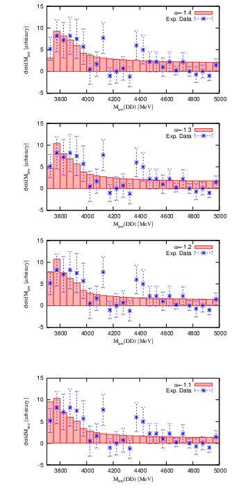
The values obtained in table 1 are around 1 or below, indicating a good fit to the data in all curves. This is in part due to the large experimental errors, but the clear message is that the presence of a pole below the threshold is enough to reproduce the observed enhancement of the cross section for this reaction in the invariant mass above threshold. The results of table 1 and inspection of fig. 3 show some preference for values of =-1.3, -1.2, which would correspond to the hidden charm scalar with mass slightly above 3700 MeV.
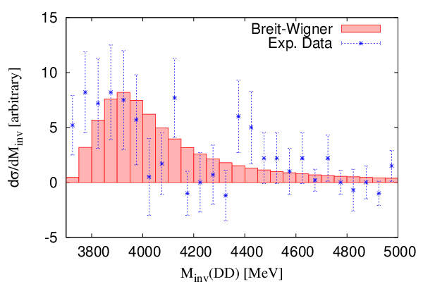
The peak seen in the experiment has been fitted with a Breit-Wigner like resonance in [29], suggesting a new resonance. In order to make the results obtained here more meaningful, we also perform such a fit and compare the results. We take the same Breit-Wigner parameters suggested in the experimental paper, =3878 MeV and =347 MeV. We show the results obtained by fitting a Breit-Wigner form from eq. (2) in of eq. (3) in fig. 4. Additionally we calculate and find =2.10 for the distribution. The value of for the distribution can be improved if we take different parameters for the Breit-Wigner resonance. Taking for the fit =3750 MeV and =250 MeV we obtain a value of =1.12, still slightly bigger than those obtained in our previous analysis assuming the mechanism of fig. 2 driven by the scalar state.
As a consequence of the discussion, our conclusions would be that for the case of the broad peak seen in , the weak case in favor of a new state around 3880 MeV discussed in [29] is further weakened by the analysis done here, showing that the results are compatible with the presence of a scalar hidden charm state with mass around 3700 MeV.
5 Dynamically generated axial vector mesons with open and hidden charm
With the interaction of pseudoscalar mesons with vector mesons in [23] one obtains the results shown in Table 2. In addition to the well known , , and (and all those in the light sector already found in [16, 17]) one obtains new states, which could be observed, although some of them are either too broad or correspond to cusps.
Table 2: Pole positions for the model. The column Irrep shows the results in the limit. The results in brackets for the are obtained taking into account the finite width of the and mesons.
| C | Irrep | S | I | RE() | IM() | Resonance ID |
|---|---|---|---|---|---|---|
| Mass (MeV) | (MeV) | (MeV) | ||||
| 1 | 1 | 0 | 2455.91 | 0 | ||
| 2432.63 | 0 | 2311.24 | -115.68 | |||
| 6 | 1 | 1 | 2529.30 | -238.56 | (?) | |
| 2532.57 | 0 | Cusp (2607) | Broad | (?) | ||
| -i199.36 | -1 | 0 | Cusp (2503) | Broad | (?) | |
| 1 | 0 | 2573.62 | -0.07 [-0.07] | |||
| 2535.07 | 0 | 2526.47 | -0.08 [-13] | |||
| -i0.08 | ||||||
| 6 | 1 | 1 | 2756.52 | -32.95 [cusp] | (?) | |
| Cusp (2700) | 0 | 2750.22 | -99.91 [-101] | (?) | ||
| Narrow | -1 | 0 | 2756.08 | -2.15 [-92] | (?) | |
| 0 | 1 | 0 | 0 | 3837.57 | -0.00 | |
| 3867.59 | ||||||
| 1 | 0 | 0 | 3840.69 | -1.60 | (?) | |
| 3864.62 |
Very interesting and novel in the present approach is the generation of the X(3872) with positive C-parity and another state nearly degenerate with negative C-parity. It would be interesting to see if a state with negative C-parity is observed, but the large branching fraction
| (6) |
indicates either a very large G-parity (isospin) violation (quite unlikely), or the existence of another state with different C-parity (G-parity also in this case).
6 Dynamically generated baryon states from the interaction of two mesons and one baryon
We discussed before how the low lying baryon resonances appear dynamically generated in the chiral unitary approach. The low lying resonances are not less problematic and quark models have difficulties in reproducing them [31]. Experimentally some of them are poorly understood and few of them possess four-star status. Among the rest some resonances are listed with unknown spin parity and two are controversial in nature. The situation is slightly better with the resonances in the same energy region, except for the (1600) and (1810), where the peak positions and widths, obtained by different partial wave analysis groups, vary a lot. Many of these S= states seem to have significant branching ratios for three-body, i.e., two meson-one baryon, decay channels. However, no theoretical attempt has been made to study the three body structure of these resonances, until recently when a coupled channel calculation for two meson one baryon system was carried out using chiral dynamics [32, 33].
7 Formalism for the three body systems
We take advantage of the fact that there are strong correlations in the meson baryon sector in L=0, and with S= one obtains many resonances. The () couples strongly to the and its coupled channels. Considering this we build the three body coupled channels by adding a pion to combinations of a pseudoscalar meson of the SU(3) octet and a baryon of the octet which couple to . For the total charge zero of the three body system we get twenty-two coupled channels. Details can be seen in [32, 33].
To solve the Faddeev equations we write the two body -matrices using unitary chiral dynamics. These -matrices can be split into an on-shell part, depending only on the respective center of mass energy, and an off-shell part, which is inversely proportional to the propagator of the off-shell particle. This off-shell part cancels a propagator in the three body scattering diagrams, leading to a diagram with a topological structure equivalent to that of a three body force [32, 33]. To this, one must add the three body forces originating directly from the chiral Lagrangians. Interestingly, in our case, we find that the three body forces from the two sources cancel in the SU(3) limit. In a realistic case, we find them to sum-up to merely 5 % of the total on-shell contribution of the -matrices to the Faddeev equations. The formalism is thus developed further in terms of the on-shell parts of the two body -matrices.
We begin with Faddeev equations
| (7) |
which, if iterated while neglecting the terms with , corresponding to the disconnected diagrams, will give
In order to convert the Faddeev equations into a set of algebraic equations one writes the terms with three successive interactions explicitly, which already involve a loop evaluation. One finds technically how to go from the diagrams with two interactions to those with three interactions and the algorithm found is then used for the next iterations, leading thus to a set of algebraic equations, which are solved within twenty two coupled channels.
The resulting Faddeev equations have been solved with the input two body -matrices obtained by solving the Bethe-Salpeter equation as in [3, 8, 34]. We find four and two states as dynamically generated resonances from a two meson-one baryon system, which we associate to known resonances of the PDG [35], implying a strong coupling of the S= resonances, in this region, to the three body decay channels. In Fig. 5 we plot the modulus square of the T-matrix as a function of two variables, the total energy and the invariant mass of particles two and three. We show results for one of the resonances, corresponding to the (1660) [35] found in our study in the squared amplitude for the channel, and in fig. 6 we show the results for the . In addition to this, we find evidence for (1) another resonance, i.e., the (1770), (2) for the controversial (1620) and (3) for the (1560), which is listed with unknown spin-parity [35]. In the isospin 0 sector we find evidence for the (1600) and (1810).
In a recent paper [36] the work has been extended to the sector with . There one finds neatly the as a resonant state of , but the Roper does not show up, indicating a far more complicated structure, as one may guess from the study of [37], where the , and channels, with interactions additional to those used in the approach of [36] are considered. In this paper one can find in detail the cancellations between the off shell parts of the amplitudes and the three body forces coming from the chiral Lagrangians that we have mentioned above. The signal for the is seen in fig. 7.


Finally we would like to report on the recent work on the generation of the X(2175) resonance found at BABAR in the [38, 39] and also confirmed at BES in the study of the decay mode [40]. The work has been done in [41] with the same three body scheme using the particles . A neat resonance is found around 2150 MeV with a width compatible with experiment, see fig. 8. As mentioned above, we plot the modulus square of the matrix as a function of two variables, the total energy and the invariant mass of the subsystem. We not only find the mass on the right place, but we also find the peak of the invariant mass at the position, indicating that the system of three particles is strongly correlated in a and the as found in the experiment.

In this latter work we also evaluated the quantitative effect of cancellation of the off-shell part of the amplitudes with the three body forces. If the later are omitted, keeping the off shell dependence of the amplitudes, the peak still appears but shifted by 40 MeV at lower energies. The cancellation between the off shell terms of the amplitudes and the three body forces has thus a nontrivial consequence if omitted. If we look at it from a different perspective, we can say that should one had used the full off shell extrapolation of the amplitudes one would have to add the effects of the three body force, which in this case would induce a shift of 40 MeV in the mass of the resonance.
To conclude, we are finding a new picture for the low lying baryon states with , which largely correspond to bound states or resonances of two mesons and a baryon. In the sector we find a clear signal for the , which has a very large branching ratio for decay into in the PDG, but not for the . This negative result for the Roper should rather be interpreted in positive terms as a clear indication that the that we study is not the most important component of the Roper structure, hinting, together with the study of [37], at a very complex structure for the . In the three meson sector a clear peak could be seen for the three body interacting system , strongly correlated around the , reflecting the strong coupling of the resonance to , the main building block of the as a dynamically generated resonance.
Acknowledgments
L. S. Geng wishes to acknowledge support from the Ministerio de Educacion in the program of Doctores y Tecnologos extranjeros and D. Strottman in the one of sabbatical. A. Martinez and D. Gamermann from the Ministry of Education and Science and K. Khemchandani from the HADRONTH project for the EU. This work is partly supported by DGICYT Contract No. BFM2003-00856, FPA2007-62777 and the E.U. FLAVIAnet network Contract No. HPRN-CT-2002-00311. This research is part of the EU Integrated Infrastructure Initiative Hadron Physics Project under Contract No. RII3-CT-2004-506078. The work of M. N. was supported by CONACyT México under project 50471-F.
References
- [1] J. Gasser and H. Leutwyler, Nucl. Phys. B 250, 465 (1985).
- [2] U. G. Meissner, Rept. Prog. Phys. 56, 903 (1993) .
- [3] J. A. Oller and E. Oset, Nucl. Phys. A 620, 438 (1997) [Erratum-ibid. A 652, 407 (1999)] .
- [4] J. A. Oller and E. Oset, Phys. Rev. D 60 (1999) 074023 [arXiv:hep-ph/9809337].
- [5] J. A. Oller, E. Oset and J. R. Pelaez, Phys. Rev. D 59, 074001 (1999) [Erratum-ibid. D 60, 099906 (1999)] .
- [6] J. R. Pelaez, Phys. Rev. Lett. 92 (2004) 102001 [arXiv:hep-ph/0309292].
- [7] N. Kaiser, P. B. Siegel and W. Weise, Nucl. Phys. A 594 (1995) 325 .
- [8] E. Oset and A. Ramos, Nucl. Phys. A 635 (1998) 99 .
- [9] J. A. Oller and U. G. Meissner, Phys. Lett. B 500 (2001) 263 .
- [10] C. Garcia-Recio, M. F. M. Lutz and J. Nieves, Phys. Lett. B 582 (2004) 49 .
- [11] D. Jido, J. A. Oller, E. Oset, A. Ramos and U. G. Meissner, Nucl. Phys. A 725 (2003) 181 .
- [12] J. A. Oller, Eur. Phys. J. A 28 (2006) 63 [arXiv:hep-ph/0603134].
- [13] E. E. Kolomeitsev and M. F. M. Lutz, Phys. Lett. B 585 (2004) 243 .
- [14] S. Sarkar, E. Oset and M. J. Vicente Vacas, Nucl. Phys. A 750 (2005) 294 [Erratum-ibid. A 780 (2006) 78] .
- [15] C. Garcia-Recio, J. Nieves and L. L. Salcedo, Phys. Rev. D 74 (2006) 034025 .
- [16] M. F. M. Lutz and E. E. Kolomeitsev, Nucl. Phys. A 730 (2004) 392 .
- [17] L. Roca, E. Oset and J. Singh, Phys. Rev. D 72, 014002 (2005) .
- [18] E. E. Kolomeitsev and M. F. M. Lutz, Phys. Lett. B 582 (2004) 39 .
- [19] J. Hofmann and M. F. M. Lutz, Nucl. Phys. A 733 (2004) 142 .
- [20] F. K. Guo, P. N. Shen, H. C. Chiang and R. G. Ping, Phys. Lett. B 641 (2006) 278 [arXiv:hep-ph/0603072].
- [21] D. Gamermann, E. Oset, D. Strottman and M. J. Vicente Vacas, Phys. Rev. D 76 (2007) 074016 .
- [22] F. K. M. Guo, P. N. M. Shen and H. C. M. Chiang, Phys. Lett. B 647 (2007) 133 .
- [23] D. Gamermann and E. Oset, Eur. Phys. J. A 33 (2007) 119 .
- [24] L. S. Geng, E. Oset, L. Roca and J. A. Oller, Phys. Rev. D 75 (2007) 014017 .
- [25] C. Daum et al. [ACCMOR Collaboration], Nucl. Phys. B 187, 1 (1981).
- [26] J. Hofmann and M. F. M. Lutz, Nucl. Phys. A 763 (2005) 90 .
- [27] T. Mizutani and A. Ramos, Phys. Rev. C 74 (2006) 065201 .
- [28] H. Walliser, Nucl. Phys. A 548 (1992) 649.
- [29] K. Abe et al. [Belle Collaboration], arXiv:0708.3812 [hep-ex].
- [30] D. Gamermann and E. Oset, Eur. Phys. J. A, arXiv:0712.1758 [hep-ph].
- [31] L. Y. Glozman and D. O. Riska, Phys. Rept. 268 (1996) 263 [arXiv:hep-ph/9505422].
- [32] A. Martinez Torres, K.P. Khemchandani and E. Oset, Eur. Phys. J. A35 (2008) 295.
- [33] A. Martinez Torres, K. P. Khemchandani and E. Oset, Phys. Rev. C 77 (2008) 042203 [arXiv:0706.2330 [nucl-th]].
- [34] T. Inoue et. al., Phys. Rev. C 65. 035204 (2002).
- [35] W.-M. Yao et al., J. Phys. G 33, 1 (2006).
- [36] K. P. Khemchandani, A. M. Torres and E. Oset, arXiv:0804.4670 [nucl-th].
- [37] O. Krehl, C. Hanhart, S. Krewald and J. Speth, Phys. Rev. C 62 (2000) 025207 [arXiv:nucl-th/9911080].
- [38] B. Aubert et al. [BABAR Collaboration], Phys. Rev. D 74 (2006) 091103 [arXiv:hep-ex/0610018].
- [39] B. Aubert et al. [BABAR Collaboration], Phys. Rev. D 76 (2007) 012008.
- [40] M. Ablikim et al. [BES Collaboration], Phys. Rev. Lett. 100 (2008) 102003.
- [41] A. Martinez Torres, K. P. Khemchandani, L. S. Geng, M. Napsuciale and E. Oset, arXiv:0801.3635 [nucl-th].