Exact many-electron ground states
on diamond and triangle Hubbard
chains
Abstract
We construct exact ground states of interacting electrons on triangle and diamond Hubbard chains. The construction requires (i) a rewriting of the Hamiltonian into positive semidefinite form, (ii) the construction of a many-electron ground state of this Hamiltonian, and (iii) the proof of the uniqueness of the ground state. This approach works in any dimension, requires no integrability of the model, and only demands sufficiently many microscopic parameters in the Hamiltonian which have to fulfill certain relations. The scheme is first employed to construct exact ground state for the diamond Hubbard chain in a magnetic field. These ground states are found to exhibit a wide range of properties such as flat-band ferromagnetism and correlation induced metallic, half-metallic or insulating behavior, which can be tuned by changing the magnetic flux, local potentials, or electron density. Detailed proofs of the uniqueness of the ground states are presented. By the same technique exact ground states are constructed for triangle Hubbard chains and a one-dimensional periodic Anderson model with nearest-neighbor hybridization. They permit direct comparison with results obtained by variational techniques for -electron ferromagnetism due to a flat band in CeRh3B2.
1 Introduction
Electronic correlations in solids can result in a high sensitivity of these systems to small changes in external parameters such as temperature, pressure, magnetic field, or doping [1, 2, 3]. This may then lead to strongly non-linear responses such as large resistivity and volume changes, a strong thermoelectric response, colossal magnetoresistance, and high- superconductivity. The complexity displayed by electronically correlated materials is not only the topic of fascinating fundamental research, but is also significant for technological applications, e.g., in sensors, switches, and in spintronics.
Even highly simplified models of interacting electrons are known to display a dazzling diversity of phases, e.g., metallic, insulating, and many types of long-range ordered states [4, 5]. Theoretical investigations of correlation effects almost always make some kind of approximation which cannot, in general, explain the full complexity of a model in detail. In this situation exact solutions of correlation models are particularly important and useful.
In this paper we discuss a general strategy for the construction of exact many-electron ground states of lattice models such as the Hubbard model. The approach is based on three distinct steps: (i) the rewriting of the Hamiltonian in positive semidefinite form, (ii) the construction of exact ground states for this Hamiltonian, and (iii) the proof of the uniqueness of the ground states constructed thereby.
This strategy was recently employed to construct a class of exact ground states of a three-dimensional periodic Anderson model (PAM), including the conventional PAM on regular Bravais lattices at and above 3/4 filling [6, 7], and to the diamond Hubbard chain in a magnetic field [8]. In both cases a wide range of features such as metallic, non-Fermi liquid, and insulating phases in the case of the PAM [6, 7], and flat-band ferromagnetism, correlation-induced metallic, half-metallic, or insulating behavior in the case of the diamond Hubbard chain [8] was found. These exact results prove that the phase diagram of even seemingly simple quantum mechanical models of many-particle systems can indeed be surprisingly complex.
The construction of exact ground states by casting the Hamiltonian into positive semidefinite form was originally applied by Brand and Giesekus to the Hubbard model and the PAM on special perovskite-type decorated lattices in dimensions at [9]. The procedure was generalized by Strack [10] to the PAM and the extended Emery model on regular lattices in low dimensions [11], and to the extended Hubbard model. The method was subsequently used to derive rigorous criteria for the stability of saturated ferromagnetism in general Hubbard-type models [12]. The possibility of superconductivity in the extended Hubbard model and its strong coupling limit was also investigated [13, 14, 15]. Furthermore, next-nearest neighbor terms in the Hamiltonian were shown to cause charge density waves, degenerate non-magnetic localized phases, and phase separation [16]. Introducing operators to rewrite the Hamiltonian in positive semidefinite form which are defined on the entire unit cell of a -dimensional lattice (e.g., on plaquettes in or cubes in ) rather than only on bonds, Orlik and Gulácsi [17] investigated the PAM on regular two- and three-dimensional lattices at , finding insulating non-magnetic phases. This method was used by Sarasua and Continentino [18] to analyze the one-dimensional PAM in more detail. Gurin and Gulácsi [19] and Gulácsi [20] demonstrated that it is also possible to investigate the PAM in at . The exact ground states constructed by Gulácsi and Vollhardt for the PAM at [6] and [7] gave the first mathematical proof for the presence of ferromagnetism in this model in dimension . These authors also detected a strong anomaly in the compressibility of the system at the boundary of the parameter region where the non-magnetic localized phase is stable — a feature which is typical for electron systems such as Cerium. In this connection the uniqueness of the constructed states was proved explicitly for the first time.
Most recently, the present authors constructed exact ground states of interacting electrons on the diamond Hubbard chain in a magnetic field [8]. This model was shown to exhibit a wide range of properties such as flat-band ferromagnetism and correlation induced metallic, half-metallic or insulating behavior which can be tuned by changing the magnetic flux, local potentials, or the electron density.
In this paper we present details of the construction of exact many-electron ground states on the diamond Hubbard chain and of their physical properties [8]. In particular, in the Appendices A and B we provide details of the mathematical proof of the uniqueness of the ground-state solutions for this model. We also construct exact ground states on triangle Hubard chains and show that within a particular subspace of parameters the triangle Hubbard chain may be mapped to a one-dimensional PAM. The exact solutions obtained for this model can be applied to investigate the correlated electron material CeRh3B2, for which Kono and Kuramoto [21] had constructed an approximate solution.
The paper is structured as follows: In Sec. 2 we discuss the general strategy for the construction of exact many-electron ground states. Exact ground states are constructed for the diamond Hubbard chain in Sec. 3. Details of the proof of the uniqueness of these ground states are presented in the appendices A and B. The technique is employed in Sec. 4 to obtain exact ground states also for the triangle Hubbard chain, and the results are applied to explain properties of CeRh3B2.
2 Construction of exact many-electron ground states: General Strategy
Our construction of exact many-electron ground states is based on the following three steps.
2.1 Step 1: Rewriting the Hamiltonian in positive semidefinite form
In the first step the many-electron Hamiltonian is cast into positive semidefinite form. This means that one rewrites the Hamiltonian in terms of a number of positive semidefinite operators as
| (1) |
where is the ground-state energy. Here (1) is supposed to be an operator identity, involving no approximations. The positive semidefinite nature of is expressed by the relation , which must be satisfied for all . Due to this inequality, the minimal eigenvalue of is zero. This property, i.e., the existence of a well-defined lower bound, namely zero, in the spectrum of in (1) is the corner stone of the procedure. Simple examples for a positive semidefinite operator are , or , or , where the positive semidefinite operator assumes its minimum eigenvalue if at least one electron is present on the site .
The scalar in (1), i.e., the ground state energy, is usually a complicated function of the parameters entering in . It should be noted that the decomposition of in positive semidefinite form is, in general, not unique and can be obtained in different ways. Each transformation is valid only in certain parts of the parameter space.
2.2 Step 2: Construction of the exact many-electron ground states
After the transformation of a given Hamiltonian into a particular positive semidefinite form valid in a parameter space region , the exact ground state of needs to be constructed. Since , and the minimal eigenvalue of each is zero, this requires the construction of the most general state which satisfies
| (2) |
for all . Consequently,
| (3) |
holds, where is the ground state, with as the ground state energy in . The actual construction of depends on the explicit expression of the operators in (1). Therefore each case must be individually analyzed. Nevertheless the following guideline may be applied (here we restrict ourselves to fermionic particles):
i) For operators the ground state has, in general, the form , where is the vacuum, and the anti-commutation relation holds. Indeed, in this case one has . To construct the global ground state one then tries to extend this property to all operators .
ii) Likewise, for operators the ground state construction makes use of and starts from states of the form , since in this case . To obtain from the property , valid for a particular , must be extended to all operators .
2.3 Step 3: Proof of the uniqueness of the ground states
Finally the constructed ground state has to be shown to be unique, i.e., one must prove that there exist no other linearly independent eigenstates of in with the same energy . This step employs the property of the kernel of which is defined as the Hilbert subspace of states with , e.g.
| (4) |
Since , one has . To prove the uniqueness one must
show that spans . For this it is
necessary and sufficient to prove that
(i) is an element of the intersection of the
kernels of all positive semidefinite operators , i.e.,
, and that
(ii) all states can
be written in terms of the constructed ground state
.
We note that if condition (ii) is not satisfied the constructed ground state is not unique, implying that other, linearly independent states with the same lowest energy exist. The uniqueness of the ground states constructed in this paper is proved in Appendices A and B.
2.4 Discussion
The procedure described above works, in principle, in any dimension and for any model, independent of the concept of integrability. On the other hand, a decomposition of into positive semidefinite form and a subsequent construction of the ground state may not always be possible — especially for Hamiltonians with a very simple structure. Indeed, the procedure works the better the more microscopic parameters (e.g., hopping amplitudes, bands, etc.) enter in . This is due to the fact that in a high-dimensional parameter space it is easier to find a subspace where a relation between microscopic parameters is found, for which the transformation of the Hamiltonian into positive semidefinite form holds.
3 Exact many-electron ground states on diamond Hubbard chains

The first exact many-electron ground states for the diamond Hubbard chain in an external magnetic field have been deduced by Gulácsi, Kampf, and Vollhardt [8]. Here we provide further details of the construction process and the physical properties of this system.
The diamond Hubbard chain is shown in Fig. 1. This chain has 3 sites per unit cell, hence 3 sublattices, denoted by the sublattice index , and therefore 3 bands. One denotes by , and the number of electrons, cells, and electron density, respectively. The Hamiltonian of the chain is given by
| (5) | |||||
| (6) |

In the external magnetic field the hopping matrix elements acquire the Peierls phase factor with and is the flux quantum. Here we have chosen the vector potential , and the field dependent hopping amplitudes follow from . For one flux quantum per unit cell (triangle) . The Zeeman term is not explicitly included in , but all deduced ground states have also been analyzed in the presence of the Zeeman term.
Fourier transforming one finds , where the matrix elements , which determine the free-electron dispersion, are given in Ref.[8]. In the following all energies will be given in units of . Examples for bare band structures are schematically shown in Fig. 2.
3.1 Flat-band ferromagnetism

We first consider the parameters , in which case the single-electron band structure consists of three flat bands (see Fig. 2a). This corresponds to the ”Aharonov-Bohm cage” limit analyzed by Vidal et al. [22] for the two electron problem with (see also Fig. 3). Based on their finding that excited singlet eigenstates are localized for but delocalized for , Vidal et al. conjectured that such delocalized states should emerge also at finite electron densities. Below we deduce indeed exact ground states for the diamond Hubbard chain at finite densities.
Following the strategy outlined in §2 one first transforms the kinetic part of the Hamiltonian into positive semidefinite form by introducing new canonical fermionic operators in real space (for details see Ref.[8]); these operators represent localized Wannier eigenstates (see Fig. 3). With the energies , one obtains
| (7) |
Since and are positive semidefinite operators the ground state of for , becomes
| (8) |
For one obtains a fully saturated ferromagnetic ground state in the lowest band (see Fig. 4) which represents an explicit realization of Mielke-Tasaki’s flat band ferromagnetism [23]. The strategy for the proof of the uniqueness of this ground state is discussed in Appendix A. For only the Wannier states with a spatial overlap have the same spin, the (highly degenerate) ground state hence consists of ferromagnetic clusters of arbitrary spin orientation. Since and the kinetic part of is diagonal in real space, the ground state (8) is localized. The explicit proof of the uniqueness of (8) for is presented in Appendix B.
The flat-band ferromagnetism found here realizes early ideas of Gutzwiller[24] and Kanamori[25] from 1963 about the origin of ferromagnetism. They argued that the ferromagnetic orientation of the electronic spins is due to the fact that the local interaction is thereby completely suppressed thus lowering the energy greatly.

However, they were not able to compute the associated loss in kinetic energy of this highly correlated state. In the present case of flat-band ferromagnetism the latter effect poses no problem since the kinetic energy is zero anyway.
We note that at the lowest band is flat only for , but is dispersive for , or . In the latter situation the system is most probably conducting for incommensurate fillings. Hence one encounters here a magnetic field induced metal-insulator transition.
3.2 Correlated half-metal
The previous results suggest that itinerant states are easier to realize at . To analyze this problem we investigate below the special case , , and ; the single-electron band structure has a dispersive lowest band and two upper flat bands (see Fig. 2b).
3.2.1 Transformation of into positive semidefinite form
For the rewriting of one defines first the non-canonical fermionic operators
| (9) |
which fulfill and . Based on (9) one obtains
| (10) | |||||
As discussed in Sec. 2.2. the coefficients , , , can be determined in different ways, namely by either requiring or . Here we choose the former condition which will enable us to construct exact ground states for (see Sec. 3.2.2.). With the requirement one arrives at the matching conditions
| (11) |
from which
| (12) |
follows. Based on (10 -12), is rewritten as
| (13) |
For the interaction part , one uses
| (14) |
is the particle number operator, and is a positive semidefinite operator, which gives zero for at least one electron on site and 1 for an unoccupied site . Consequently, has been transformed into the positive semidefinite form
| (15) |
where .
3.2.2 Construction of the ground state
As discussed in Sec. 2.2, the ground state for is deduced such to satisfy and , from where indeed
| (16) |
follows. Since one finds
| (17) |
In order to satisfy as well, which requires one electron on each site, besides the contribution from (17) one has to introduce in the ground state wavefunction also the operator
| (18) |
which creates two electrons with fixed spin on arbitrary sites of each unit cell. Hence, the unnormalized ground state becomes
| (19) |
where is a normalization constant. The contribution in (17) creates one electron, and an electron with spin in each unit cell, while creates two electrons with spin on arbitrary sites of each unit cell. Consequently the ground state in (19) corresponds to , , , . The proof of the uniqueness of (19) is presented in detail in Appendix A. In conclusion, (19) is the unique ground state.
Concerning the physical properties of the ground state one observes that in (19) each lattice site is occupied by one -electron; hence, the -electrons are localized. The electrons are spatially extended, but localized for . This is inferred from the ground-state expectation value of the hopping term , which in the limit , for , is calculated as
| (20) |
The one-particle localization length in (20) increases almost linearly with [8].
3.2.3 Solution for
For electron densities there are electrons. No -electrons but -electrons can be added to the system such that , . The ground state then becomes
| (21) |
where can be arbitrarily chosen from . Eq. (21) contains plane wave-type contributions from the -electrons. Consequently, the additional electrons are itinerant. Indeed, this follows explicit from the expectation value of the hopping term . For , , , one finds . Here is the plane wave result and is the norm of the momentum of the electron added above . We note that the momenta in (21) are arbitrary. Hence it is not possible to define a Fermi surface, and the ground state therefore corresponds to a non-Fermi liquid.
In the density range the ground state has immobile electrons and electrons with spin confined to their localized Wannier functions. For this reason the ground state has a high geometric degeneracy; its uniqueness is discussed in Appendix B.
Only the conducting electrons are itinerant, leading to metallic behavior with a low carrier density and a low spin polarization. Since the conduction through this correlated half-metal involves only electrons of one spin species, such a system may serve as a spin-valve device. Since is required for this property one encounters here a correlation induced localization-delocalization transition to a half-metal. The magnetization behaves as for . in a finite magnetic field. The transition can also be induced by tuning the local potential . At the ground state becomes nonmagnetic and localized in the thermodynamic limit, while at one finds a nonmagnetic but conducting ground state.
3.3 Exact ground states for general magnetic flux
It is also possible to construct exact ground states for general magnetic flux values including also the case, for example at with , , , , and [8]; the single-electron band structure has two dispersive bands and an upper flat band (see Fig. 2c). For these hopping and potential parameters one obtains a localized nonmagnetic ground state for over an extended range of densities . By contrast, at finite magnetic fields the ground state is a nonsaturated ferromagnet. This localized state at is insulating, but gapless and itinerant for . For the latter densities the majority spin -electrons are immobile and only the electrons are itinerant. Therefore, by varying the external magnetic field and the sublattice potential one can tune from a localized, nonmagnetic ground state to a nonsaturated ferromagnet in the density range ; the ferromagnetic state is insulating at , but conducting for .
We finally note the properties derived above do not depend on the Zeeman coupling. Only the solution in Sec. 3.1 for is altered by the Zeeman term, whose presence leads to a fully spin aligned ferromagnetic solution.
4 Exact many-electron ground states on triangle Hubbard chains
The procedure for the construction of exact ground states on the diamond Hubbard chain is now applied to a Hubbard chain composed of corner-sharing triangles (see Fig. 5). Triangles are well-known to frustrate non-ferromagnetic magnetic order. Hence interacting electrons on lattices with triangles as structural sub-units are expected to favor ferromagnetic ground states.

The triangle Hubbard chain in Fig. 5 has two sites per cell which leads to two energy bands. The number of electrons, cells, and electron density are here denoted by , and , respectively. This model was previously investigated in detail by Penc et al. [26], Fazekas et al. [27], Müller-Hartmann [28] and Derzhko et al. [29] with a variety of analytical and numerical techniques.
The Hamiltonian of the triangle chain has the form
| (22) |
The model parameters are explained in Fig. 5. In the following we will construct exact ground states in the subspace of parameters defined by the relation , , , for which the lowest bare band is flat.
4.1 Ground states for the triangle Hubbard chain
4.1.1 Ground state for ,

Employing the operators
| (23) |
the Hamiltonian (22) can be transformed into positive semidefinite form:
| (24) |
Here is the particle number operator and . To construct the ground state one has to find operators which satisfy for all values of the indices. The ground state then has the form
| (25) |
with , . For there exist ferromagnetic clusters, and only operators which touch have the same spin index. For all clusters touch such that a fully saturated ferromagnetic state is obtained as shown in Fig. 6a for the case. The ground state corresponds to a particular realization of flat-band ferromagnetism [23], for which Derzhko et al. [29] calculated the thermodynamic properties.
4.1.2 Ground state for ,
The ground state has the same form as (25), but now it is non-magnetic even for (see Fig. 6b). This is due to the fact that, although the connectivity condition is fulfilled (i.e., and overlap at site ) there is no interaction at the connectivity point (). The fulfillment of the connectivity condition for the Wannier functions is therefore not sufficient for the ground state to be ferromagnetic. In addition a finite Hubbard repulsion is needed at the connectivity points to guarantee a correlation between the electrons.
4.1.3 Ground state for
The ground state has again the form (25), but now it is a fully saturated ferromagnetic state at even for , since the Hubbard interaction is non-zero at the connectivity points (). We thus see that for flat-band ferromagnetism to occur the Hubbard interaction is needed only at the connectivity points. The ferromagnetic states discussed in Sec. 4.1.1 and Sec. 4.1.3. are localized in the thermodynamic limit.
4.2 Mapping to the one-dimensional periodic Anderson model (PAM)
By the following change of notation in (22)
| (26) |
and setting the triangle Hubbard chain transforms into a one-dimensional PAM with zero on-site hybridization and nearest-neighbor hybridization :
| (27) | |||||
A lowest bare flat band is obtained for , , .
4.2.1 Exact ground state for the one-dimensional PAM
In the parameter regime , , the exact ground state for the one-dimensional PAM is obtained from (25) as
| (28) |
4.2.2 Itinerant ferromagnetism of finite chains
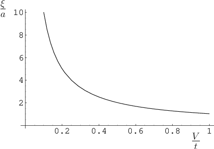
In analogy with (20) the localization length of the -electrons can be calculated from the expression for the expectation value of the hopping term . Its dependence on the nearest-neighbor hybridization strength is given by
| (29) |
as shown in Fig. 7. Here is the distance between sites at the base of the triangle chain (see Fig. 5). Although flat-band ferromagnetism in the thermodynamic limit usually corresponds to localized electrons, the localization length can be so large that it exceeds the length of a finite sample. In realistic situations the exact ground state of the finite chain therefore shows itinerant ferromagnetism.
4.3 Application to -electron ferromagnetism in CeRh3B2
As pointed out by Kono and Kuramoto [21] the one-dimensional PAM, (27), may be employed to model the -electron compound CeRh3B2. This material is ferromagnetic below K. Its properties are interesting for several reasons: (i) the ferromagnetic state cannot be explained by a RKKY interaction, (ii) the moment has the remarkably small value of 0.45 compared to the free Ce3+ moment of 2.14 , and (iii) the Curie temperature has the highest value among all known Ce compounds with non-magnetic elements.
The lattice structure of the class of rare-earth (RE) compounds RERh3B2 was determined by Yamada et al. [30]. A cut through the (a,c)-plane of the Cerium system (RE = Ce) is shown in Fig. 8. The remarkable difference between the distances of the Ce atoms along the a- and the c-direction, respectively, makes this material a quasi one-dimensional two-band system [31]. For this reason Kono and Kuramoto [21] modeled CeRh3B2 by the triangle PAM chain shown in Fig. 9. The parameters entering the model are eV, eV, eV, eV, , as obtained from band-structure calculations and X-ray absorption spectroscopy (we note that the density corresponds to twice the value, i.e., , in the notation of Ref. [21]).


4.3.1 Variational results for the one-dimensional PAM
Kono and Kuramoto [21] computed the band structure of CeRh3B2 by constructing a Gutzwiller variational wave function and using variational Monte Carlo to determine the ground state. They found the lowest band of CeRh3B2 to be almost perfectly flat and fully polarized, and the second band dispersive and almost unpolarized. It should be stressed that the shape of the lowest quasiparticle band of interacting electrons depends on .
4.3.2 Exact ground state of the one-dimensional PAM
We can use the exact ground state of the one-dimensional PAM, (28), to make direct contact with the -electron ferromagnetism found in CeRh3B2. Namely, this ground state represents a saturated flat-band ferromagnetic state of the -electrons for electron density and arbitrary , provided the condition , , holds. The condition is indeed fulfilled for the parameter values eV, eV, eV, which are very close to the experimentally determined values. In this case the lowest band is perfectly flat for all . Apparently the ferromagnetism of the -electrons in CeRh3B2 is due to the presence of an (almost) flat lowest band.
4.3.3 Magnetic moments
The experimentally observed magnetic moment of the -electrons is [32]. The variational result [21] yields , while the exact ground state discussed above leads to a value of which is even closer to the experimental value. Both theoretical values are somewhat higher than the experimental moment. This may be due to the fact that the theoretical approaches do not include the spin-orbit interaction which causes an antiferromagnetic coupling between the - and the -electrons.
5 Conclusions
Despite its simplicity, the diamond Hubbard chain displays remarkably complex physical properties with insulating, conducting, and fully or partially spin polarized states. The constructed exact many-electron ground states revealed flat-band ferromagnetism, correlated half-metallic behavior, and metal-insulator transitions in the diamond Hubbard chain. The virtue of tuning fundamentally different ground states through external magnetic fields, site selective potentials, or the electron density, points to new prospects for designing electronic devices, which allow to switch between different ground states, including states that operate as a spin valve. We applied the general strategy for the construction of exact ground states also to triangle Hubbard chains. The mapping of the triangle Hubbard chain to the one-dimensional periodic Anderson model within a restricted parameter set provided a theory for -electron ferromagnetism in CeRh3B2, which is based on the physical properties of an exact ground state.
Further applications of the construction of exact ground states by casting the Hamiltonian into positive semidefinite form are possible for model systems with selected geometries in artificially designed structures. In particular, we constructed exact ground states for pentagon Hubbard chains. These results will be presented elsewhere.
Acknowledgements
We thank F. Mila, Y. Kuramoto, and F. C. Zhang for discussions regarding the uniqueness of the solutions. Support by the Hungarian Research Fund through Contracts No. OTKA-T48782, 76821, the Alexander von Humboldt Foundation, and the Deutsche Forschungsgemeinschaft through SFB 484 is gratefully acknowledged.
Appendix A Uniqueness of ground states with where is an integer
Here we prove the uniqueness of those exact ground states constructed in this paper for which the electron number is an integer multiple of the number of unit cells . The proof proceeds as discussed in Sec. 2.3 and is exemplified by proving the uniqueness of the ground state , (19), of the diamond Hubbard chain. In this case , i.e., , and the electron density has the value . The Hamiltonian, the unnormalized ground state, and the operators entering therein are given by (15), (19), and (12), respectively. To prove the uniqueness one first has to determine the kernel of . The form of the Hamiltonian implies that its kernel is simply given by the intersection of the kernels of the individual terms, i.e., , where is an operator, which assumes its minimum eigenvalue 0, if there is at least one electron at each site.
To prove the uniqueness of the ground state , (19), it is now necessary to demonstrate that it spans . According to the discussion in Sec. 2.3 the proof consists of two parts. First one has to establish that
(i) is an element of the intersection of the kernels of the positive semidefinite operators entering in .
Then one must show that
(ii) all states from the kernel of can be written in the form of the ground state .
The first part of the proof, (i), is covered by the following Theorems A-1 to A-3. The second part of the proof, (ii), then follows immediately (see below).
To prove (i) we note that the first term in is a sum of positive semidefinite operators . The ground state of must therefore be an element of each kernel of all the operator , for all . Thus we first determine the kernel of (Sec. A.1.), then the kernel of the sum (Sec. A.2.), and finally the kernel of the full Hamiltonian (Sec. A.3.).
A.1 The kernel of
Theorem A-1: The kernel of is spanned by states of the form
| (30) |
where is an arbitrary operator.
Proof of Theorem A-1
a) From ( it follows that . This implies that .
b) In order to show that all elements of can be written in the form we consider a state and show that has the form .
Making use of and we can write
| (31) |
With the identification we have therefore verified that indeed
| (32) |
This completes the proof of Theorem A-1.
A.2 The kernel of
The kernel of has the form
| (33) |
Theorem A-2: is spanned by vectors of the form
| (34) |
where the operator is arbitrary.
Theorem A-2 follows directly from the linear independence of the operators (that is, holds for arbitrary coefficients due to the fact that the operators enter only in and not in , for .
A.3 The kernel of
The kernel of is given by , where is an operator, which assumes its minimum eigenvalue 0, if there is at least one electron at each site. Hence, is spanned by vectors of the form in Eq. (30), where now the operator is no longer arbitrary, but must have a specific form to satisfy the abovementioned requirement imposed by .
Theorem A-3: For the operator is given by , where creates two electrons with fixed spin in each unit cell.
Proof of Theorem A-3.
The proof proceeds in two main steps: we show that is 1) a possible choice, and 2) the unique choice.
1) Let us denote by the unit cell (= triangle), which contains the sites . The state has one empty site in each unit cell . We now analyze how these empty sites are filled by the product . We first observe that acts on all sites in , which implies that the empty site in can indeed be filled by applying . There are empty sites and operators ; thus, the product inserts electrons with spin into the system. Since (, the state has one -electron on all sites of the lattice. Hence, is a possible choice for in constructing the states contained in .
2) We now flip the spin of one electron in into , and denote the new operator by . In this case, a single unit cell, say , will have one empty site, one electron with spin on another site, and one electron with spin on the third site. Then the operator can create one electron with spin on the site, which already contains the electron with spin , thereby creating a double occupancy. One empty site will remain in . For , the operators can introduce their electron into the empty sites of . Hence one empty site can remain in the system. The state therefore has at least one term with an empty site and contains one electron. Acting now with on adds electrons with spin on sites. The new state will therefore have at least one term with an empty site, and is thus not an element of and . This shows that is the unique choice. This completes the proof of Theorem A-3.
Theorems A-1, A-2 and A-3 prove that , (19), is indeed an element of the intersection of the kernels of the positive semidefinite operators entering in . This completes part (i) of the proof of the uniqueness discussed in Sec. 2.3.
Appendix B Uniqueness of ground-state solutions with for non-integer
B.1 Geometric degeneracies
For non-integer as in the case of (8) for , and (21) for (as well as in the case of solution III for of Ref.[[8]]), the ground states have a high geometric degeneracy. In these cases there exist linearly independent eigenstates with the same ground-state energy. They may be denoted by a degeneracy index , where is the degree of degeneracy. The ground state then becomes where apart from the normalization condition, the coefficients are arbitrary. For these ground states the proof of uniqueness proceeds analogously to that described in Appendix A. Namely, one has to prove that spans ker(), but now, given the specific structure of , it has to be verified that
1) all linearly independent states are elements of the intersection of the kernels of the positive semidefinite operators , i.e., , and
2) all states can be written in the form of the constructed ground state, e.g. as a linear combination of the vectors .
As an example we now prove the uniqueness of the ground state , (8), for . The proof is presented for fixed , namely . For other values the proof proceeds similarly. The first part of the proof, (i), (see Sec. 2.3) is covered by the following Theorems B-1 and B-2. The second part of the proof, (ii), then follows immediately (see below).
B.2 Uniqueness of the ground state (8) for particles
The transformed Hamiltonian is determined by and as given by (7)and (6), respectively. Furthermore, one has , where are genuine canonical Fermi operators, and . Since is a constant of motion, the Hamiltonian can be written as , where and . Consequently, is a positive semidefinite operator: , where , and . The ground state is given by (8).
B.2.1 The kernel of
Theorem B-1: The kernel of is spanned by states of the form
| (35) |
where the product is taken over arbitrary sites, and is arbitrary. Note that depends on the set of sites , and the set of spin orientations .
Proof of Theorem B-1.
The proof proceeds in two steps: a) one first shows that Eq. (35) is a possible choice, and b) then verifies that it is the unique choice.
a) The initial canonical Fermi operators , where is the sublattice index, have been transformed by a linear transformation into the opertors , which satisfy canonical fermionic anti-commutation rules. Since the set of the new operators substitutes the set , all operators in the system acting on states defined by arbitrary can be expressed in terms of the operators .
Given these conditions, an operator which satisfies
| (36) |
for all indices , must have the form . Indeed, the anti-commutation relations (36) hold only for this type of operator since an arbitrary operator can be expressed in terms of operators, and only anticommutes with all and .
b) If contains at least one operator with , the relation Eq. (36) no longer holds, hence Eq. (35) is the unique choice. This proves Theorem B.1.
We furthermore observe that due to the fermionic operator nature of , the deduced elements of ker() from Eq. (35) are not only linearly independent but also orthogonal:
| (37) |
B.2.2 The kernel of
Since ker()=ker() ker(), the states in ker() have the form (35), but the specific set of indices has to be chosen such that these states are also contained in ker(). This condition requires the proof of the following theorem.
Theorem B-2: The kernel of is spanned by states of the form
| (38) |
where is fixed, and the product extends over arbitrary sites.
Since the product in Eq. (38) is taken over sites of the sublattice , the vector can be denoted by the specific site excluded from the product, i.e. . This site plays the role of the degeneracy index in Sec.B.1.
Proof of Theorem B-2.
The theorem is proved in three steps: First one has to show that all spin indices in (38) must have the same value, secondly it has to be verified that the deduced states in ker() are linearly independent, and thirdly one needs to prove that the set of the deduced states is complete.
a) All states in ker() require the absence of any double occupancy. Therefore, all indices must be fixed to the same value . The double occupancy cannot be avoided otherwise, since in unit cells operators share a common site.
b) due to the relation (37) the vectors are linearly independent, since they are orthogonal .
c) Obviously, the degree of degeneracy of a macroscopic many-body state is given by the number of equivalent configurations. Due to part a), apart from the trivial degeneracy with respect to the total spin direction, on finds , because there are possibilities for placing identical objects on sites. Consequently, ker() is an dimensional Hilbert subspace. The index in the states of the form (38) refers to possible different unit cells. Furthermore, the vectors are linearly independent, hence the set forms a (orthonormalized) basis of ker(). Therefore, spans ker(), and the ground state has the general form , with arbitrary coefficients . This proves Theorem B-2.
Since is a basis of ker(), all states can be written in the form of part c). Therefore (8) is the unique ground state of the Hamiltonian consisting of the two terms (7) and (6).
For the set is an empty set, and the upper limit set to in Eq. (38) provides the unique ground state at density (see (8) for ). A similar strategy for allows one to prove the uniqueness of the ground-state solutions for all electron densities in (8). Similar proofs are expected to hold in the case of the ground state , (21), for () and solution III for () constructed in Ref. [8].
References
- [1] M. Imada, A. Fujimori, and Y. Tokura, Rev. Mod. Phys. 70, 1039 (1998).
- [2] Y. Tokura and N. Nagaosa, Science 288, 462 (2000).
- [3] E. Dagotto, Science 309, 257 (2005).
- [4] The Hubbard Model, ed. A. Montorsi (World Scientific, Singapore, 1992).
- [5] H. Yao, W.-F. Tsai, and S. A. Kivelson; Phys. Rev. B 76, 161104(R) (2007).
- [6] Z. Gulácsi and D. Vollhardt, Phys. Rev. Lett. 91, 186401 (2003).
- [7] Z. Gulácsi and D. Vollhardt, Phys. Rev. B 72, 075130 (2005).
- [8] Z. Gulácsi, A. Kampf, and D. Vollhardt, Phys. Rev. Lett. 99, 026404 (2007)
- [9] U. Brandt and A. Giesekus, Phys. Rev. Lett. 68, 2648 (1992).
- [10] R. Strack and D. Vollhardt, Phys. Rev. Lett. 70, 2637 (1993). Physica B 199 & 200, 273 (1994).
- [11] R. Strack, Phys. Rev. Lett. 70, 833 (1993).
- [12] R. Strack and D. Vollhardt, Phys. Rev. Lett. 72, 3425 (1994); J. Low Temp. Phys. 99, 385 (1995).
- [13] A. Montorsi and D. K. Campbell, Phys. Rev. B 53, 5153 (1996).
- [14] L. G. Sarasua, Phys. Rev. B 75, 054504 (2007)
- [15] R. B. Laughlin, Phil. Mag. B 86, 1165 (2006).
- [16] P. Gurin and Z. Gulácsi, Phil. Mag. B 76, 827 (1997).
- [17] I. Orlik and Z. Gulácsi, Phil. Mag. Lett. 78, 177 (1998).
- [18] L. G. Sarasua and M. A. Continentino, Phys. Rev. B 65, 233107 (2002).
- [19] P. Gurin and Z. Gulácsi, Phys. Rev. B 64, 045118 (2001); Phys. Rev. B 65, 129901(E) (2002).
- [20] Z. Gulácsi, Phys. Rev. B 66, 165109 (2002); Eur. Phys. Jour. B 30, 295 (2002).
- [21] H. K. Kono and Y. Kuramato, J. Phys. Soc. Jpn. 75, 084706 (2006).
- [22] J. Vidal, B. Doucot, R. Mosseri, and P. Butaud, Phys. Rev. Lett. 85, 3906 (2000).
- [23] A. Mielke and H. Tasaki, Commun. Math. Phys. 158, 341 (1993).
- [24] M. C. Gutzwiller, Phys. Rev. Lett. 10, 159 (1963).
- [25] J. Kanamori, Prog. Theor. Phys. 30, 275 (1963).
- [26] K. Penc, H. Shiba, F. Mila, and T. Tsukagoshi, Phys. Rev. B 54, 4056 (1996).
- [27] P. Fazekas, Phil. Mag. B 76, 797 (1997).
- [28] E. Müller-Hartmann, J. Low Temp. Phys. 99, 349 (1995).
- [29] O. Derzhko, A. Honecker, and J. Richter, Phys. Rev. B 76, 220402(R) (2007).
- [30] M. Yamada, Y. Obiraki, T. Okubo, T. Shiromoto, Y. Kida, M. Shiimoto, H. Kohara, T. Yamamoto, D. Honda, A. Galatanu, Y. Haga, T. Takeuchi, K. Sugiyama, R. Settai, K. Kindo, S. K. Dhar, H. Harima, and Y. Onuki, J. Phys. Soc. Jpn. 73, 2266 (2004).
- [31] T. Okubo, M. Yamada, A. Thamizhavel, S. K. Y. Inada, R. Settai, H. Harima, K. Takegahara, A. Galatanu, E. Yamamoto, and Y. Onuki: J. Phys.: Condens. Mat. 15, L721 (2003).
- [32] A. Galatanu, E. Yamamoto, T. Okubo, M. Yamada, A. Thamizhavel, T. Takeuchi, K. Sugiyama, Y. Inada, and Y. Onuki, J. Phys.: Condens. Mat. 15, S2187 (2003).