Bulk viscosity in kaon-condensed color-flavor locked quark matter
Abstract
Color-flavor locked (CFL) quark matter at high densities is a color superconductor, which spontaneously breaks baryon number and chiral symmetry. Its low-energy thermodynamic and transport properties are therefore dominated by the (superfluid) boson, and the octet of pseudoscalar pseudo-Goldstone bosons of which the neutral kaon is the lightest. We study the CFL- phase, in which the stress induced by the strange quark mass causes the kaons to condense, and there is an additional ultra-light “” Goldstone boson arising from the spontaneous breaking of isospin. We compute the bulk viscosity of matter in the CFL- phase, which arises from the beta-equilibration processes and . We find that the bulk viscosity varies as , unlike the CFL phase where it is exponentially Boltzmann-suppressed by the kaon’s energy gap. However, in the temperature range of relevance for -mode damping in compact stars, the bulk viscosity in the CFL- phase turns out to be even smaller than in the uncondensed CFL phase, which already has a bulk viscosity much smaller than all other known color-superconducting quark phases.
pacs
12.38.Mh,24.85.+p,26.60.+cI Introduction
The color-flavor locked (CFL) phase of quark matter is the densest predicted state of matter [1]; it may occur in nature, in the core of compact stars, which are expected to reach several times nuclear saturation density. Quark matter is described by the theory of Quantum Chromodynamics (QCD), which, because of asymptotic freedom [2, 3], becomes weakly coupled and hence perturbatively tractable at asymptotically high densities. In that regime, the CFL phase can be shown to be the ground state. However, at compact-star densities the coupling is strong, so first-principles calculations are not possible. We therefore follow a more phenomenological approach. We start with the hypothesis that color-flavor-locked quark matter occurs in compact stars, and calculate phenomenologically relevant properties which could allow us to find astrophysical signatures of its presence. We will calculate the bulk viscosity, which is relevant for the damping of pulsations and (indirectly) the spin down of the star.
If the interior of the star is a perfect (dissipationless) fluid, then a certain class of oscillating modes, -modes, are unstable with respect to the emission of gravitational waves [4, 5, 6]. This emission acts as a brake on the rotation of the star. Since we know from observations that there are compact stars with very large rotation frequencies, we conclude that the instability must be damped. One damping mechanism is a nonzero viscosity of the fluid. Both shear and bulk viscosity can affect the -modes and typically act in different temperature regimes. Therefore, it is of physical interest to compute shear and bulk viscosity of various candidate phases in a compact star as a function of temperature. Several calculations exist in the literature, for nuclear [7, 8, 9, 10, 11, 12, 13] and hyperonic [14, 15] as well as for unpaired quark matter [16, 17, 18] and various color-superconducting phases [19, 20, 21, 22], for a review see [23]. Bulk viscosity due to thermal kaons in the CFL phase has been computed in Ref. [24]. Here, we extend this calculation to the case of condensed kaons.
At asymptotically large quark chemical potentials , three-flavor quark matter is in the CFL phase [25]. This phase breaks the local color gauge group , giving rise to Meissner masses for all eight gluons. It also breaks the global chiral symmetry group , leaving a residual global which contains simultaneous rotations in color and flavor space, hence “locking” color with flavor. Moreover, the global baryon number conservation symmetry is broken, rendering the CFL phase a superfluid. For massless quarks there are thus 8+1 massless Goldstone bosons (and an additional Goldstone boson for the symmetry, which, however, is expected to be explicitly broken at moderate chemical potentials). At moderate densities the mass of the strange quark cannot be neglected and the bosons of the octet associated with chiral symmetry breaking acquire masses. These masses are small compared to the energy gaps of the fermions, and therefore the low-energy properties of the CFL phase can be described within an effective theory for the Goldstone bosons [26, 27, 28]. We shall make use of this theory in this paper. If is large enough, it is expected that the lightest pseudo-Goldstone bosons, namely the neutral kaons, condense. The CFL phase with condensation is called the “CFL-” phase. Goldstone bosons in CFL and their condensation have also been studied in a different approach, using a Nambu-Jona-Lasinio model [29, 30, 31, 32, 33, 34].
Besides giving rise to masses for the meson octet, a nonzero strange mass induces a mismatch in the Fermi momenta of the quarks that form Cooper pairs in the CFL phase. In fact, the strange mass induces a mismatch in any possible spin-zero color-superconducting phase [35]. This means that at lower densities, the particularly symmetric CFL phase may be replaced by a less symmetric pairing pattern. It is currently not known whether, going down in density, the CFL phase is superseded by nuclear matter or by a different, more exotic, color-superconducting phase. Candidate color-superconducting phases have Cooper pairs with nonzero angular momentum [36, 37, 38, 39] or nonzero momentum [40, 41, 42]. In this paper, we shall only consider the CFL and CFL- phases.
The paper is organized as follows. In Sec. II we give a brief overview over the properties of the CFL- phase, in particular we present the low-energy excitations at finite temperature. As an application, we discuss the resulting specific heat of the system in Sec. II.5. The calculation of the bulk viscosity is presented in Sec. III. We define the bulk viscosity in Sec. III.1. In Secs. III.2 and III.3 we collect the ingredients needed for the bulk viscosity, namely the kaon density and susceptibility and the rate of the processes and . We put these ingredients together in Sec. III.4 to obtain the result for the bulk viscosity and give our conclusions in Sec. IV.
II Low-energy modes in the CFL- phase
In this section, we briefly summarize the theoretical description and physical properties of the Goldstone bosons in the CFL- phase. More details can be found in the references given in the text.
II.1 Chiral Lagrangian
We denote the meson nonet in the CFL phase, associated with chiral symmetry breaking, by
| (1) |
where is an element of the Lie algebra of . The physics of the mesons is described by the Lagrangian [27, 26]
| (2) |
There is an effective chemical potential given by the “gauge field”
| (3) |
where and are the electric charge and quark mass matrices in flavor space, and is the chemical potential associated with electric charge. Moreover, from matching calculations at asymptotically large densities we know
| (4) |
where is the fermionic energy gap at zero temperature. It turns out that the neutral and charged kaons are the lightest mesons. They carry flavor quantum numbers , , , . In contrast to the usual mesons, however, they are composed of four quarks of the structure as opposed to . The zero-temperature kaon masses and effective chemical potentials are deduced from the Lagrangian and are given by
| (5a) | |||||
| (5b) | |||||
We see that with slightly larger than the neutral kaon is slightly lighter than the charged kaon. Moreover, electric neutrality disfavors the presence of charged kaons. Therefore, in most of the remainder of the paper we shall ignore the charged kaons. In the following, for notational convenience, we denote the neutral kaon chemical potential and mass simply by and , respectively,
| (6) |
Condensation of the neutral kaons occurs if . Because of the large uncertainty in the quark masses and in the dimensionless quantity , it is not clear whether this condition is fulfilled for densities present in the interior of a compact star. Using the high-density expressions in Eq. (4) and inserting a quark chemical potential and an energy gap , we estimate , . With , we thus obtain a kaon chemical potential and a kaon mass . These values suggest that the kaons are condensed and thus that the relevant phase to consider is the CFL- phase. It has been argued that for sufficiently large values of the parameter the CFL- phase is modified to the so-called curCFL- phase which is anisotropic and exhibits counter-propagating currents from the kaon condensate and ungapped fermions [43, 44, 45]. Because of the presence of ungapped fermions, the transport properties of this phase can be expected to be very different from the ones in the CFL- phase and similar to unpaired quark matter. In this paper, we do not consider the possibility of a kaon current but rather focus on the isotropic CFL- phase where all fermions are gapped.
II.2 2PI formalism for kaons
To obtain the Lagrangian for the neutral kaons in the presence of a kaon condensate we start from the Lagrangian (2) and set
| (7) |
where , are Gell-Mann matrices. We have omitted the other Goldstone modes, proportional to , and have introduced a vacuum expectation value for the kaon field (without loss of generality in the direction) and fluctuations , with vanishing expectation value. The Lagrangian is now expanded up to fourth order in the fluctuations. See Ref. [46] for details and the explicit form of the Lagrangian. The tree-level potential is
| (8) |
where we have abbreviated the effective coupling constant
| (9) |
In principle, one can keep all orders in , but for simplicity we have expanded for small values of . This restricts our analysis to small condensates. In other words, our results are quantitatively reliable if is only slightly larger than and become unreliable for . In addition to the tree-level potential, the Lagrangian contains quadratic terms in the fluctuations from which we read off the inverse tree-level propagator
Here and in the following we denote four-momenta by capital letters , where the bosonic Matsubara frequencies are given by with the temperature . The Lagrangian also contains interaction terms cubic and quartic in the fluctuations. For small condensates we may neglect the cubic interactions. The form of the quartic interactions is needed for the vertex in the kaon self-energy.
The nonzero-temperature behavior of systems with spontaneously broken symmetries can be conveniently treated within the two-particle irreducible (2PI) formalism [47, 48, 49]; for the application of this formalism in chiral models see for instance Refs. [50, 51, 52]. Naive thermal corrections would lead to unphysical results for a Bose-condensed system, in particular to negative energies for certain temperature regimes. Therefore, we apply the more elaborate 2PI scheme to compute the thermal masses self-consistently. We start from the effective potential
| (13) |
where the trace is taken over momentum space and over the two-dimensional space given by the two degrees of freedom of the kaon (corresponding to and or and ). The effective potential is a functional of the vacuum expectation value and the kaon propagator . The term is the sum over all 2PI diagrams. We employ the two-loop approximation for this infinite sum and only consider the “double-bubble” diagram, see Fig. 1. In this case does not explicitly depend on .

One can now determine the condensate and the thermal kaon mass self-consistently. This is done by solving the stationarity equations
| (14a) | |||||
| (14b) | |||||
where is the kaon self-energy, see Fig. 1. With the ansatz for the full inverse propagator
the stationarity equations read
| (18a) | |||||
| (18b) | |||||
Here, is the temperature dependent mass, related to in the propagator (II.2) by . The other combination can be eliminated since the second matrix component of Eq. (14b) implies .11 1 In fact we have with being a momentum integral similar to in Eq. (19). We may neglect the term . This removes a very small mass for the Goldstone boson, which arises as an artefact in the 2PI formalism at finite temperature. For details and the expression for see Ref. [46]. We have abbreviated
| (19) |
with
| (20) |
and the Bose distribution function
| (21) |
The kaon excitation energy is a pole of the propagator (II.2). Its form is crucial for the thermodynamic and transport properties of the CFL- phase and will be discussed explicitly in Sec. II.3, see Eq. (23). The second pole of the propagator corresponds to the excitation. This excitation has a (temperature-dependent) energy gap which is larger than the excitation by at least . We will neglect the mode in our analysis, because is expected to be on the order of , so the would only play a role at temperatures in the tens of MeV range. This is close to the critical temperature of the CFL phase itself, and is not physically relevant because compact stars cool below such temperatures within minutes of their formation. Our results are therefore reliable at temperatures of order 1 MeV or lower. In some cases we will continue our expressions to higher temperatures: this represents a theoretical exercise in studying the properties of the pure condensate, not a physical prediction.
For the calculations of the specific heat in Sec. II.5 as well as for the density and susceptibility in Sec. III.2 we need an explicit expression for the pressure which is the negative of the effective potential (13), . In the given approximation we can write as a function of and ,
| (22) |
The pressure in the physical state is then given by inserting the values for and at the stationary point.
II.3 Kaon excitation energies
For the calculation of transport properties we are interested in the kaon dispersion relations which are the poles of the propagator (II.2). Dropping the excitation, see remark below Eq. (21), the only relevant kaon dispersion relation is [46]
| (23) |
with determined from the stationarity equations (18). We have eliminated from the expression for by using Eq. (18a). The critical temperature of the second-order phase transition for kaon condensation is denoted by , i.e., for temperatures below (above) we have (). The value of is estimated to be at least of the order of tens of MeV [46]. This shows that for all temperatures relevant for compact stars, the kaons will be condensed (provided the parameters and are such that there is condensation at zero temperature). The self-consistent treatment ensures that for all temperatures , and thus the energies given in Eq. (23) are real and positive as they should be. Moreover, from Eq. (23) we see that for . This shows that there is a massless Goldstone mode associated with kaon condensation.22 2 We shall in the following use the term for this Goldstone mode in the CFL- phase as well as for the member of the meson octet arising from chiral symmetry breaking in the CFL phase. This is the most convenient terminology but one should keep in mind that these two excitations have very different dispersion relations. It is the presence of this gapless mode that causes thermodynamic and transport properties of the CFL- phase to differ from those of the CFL phase. Strictly speaking, this Goldstone mode also has a small energy gap. This energy gap does not show up in our treatment within the effective theory given by the Lagrangian (2). The energy gap is rather induced by the weak interactions and can be estimated to be in the keV range [53]. Most of the temperature scales we show in this paper do not include temperatures below this range. Therefore, we shall neglect this effect and speak of an exact Goldstone mode with massless dispersion relation given by Eq. (23).
It is instructive to expand the kaon dispersion below for small momenta,
| (24) |
For small momenta, the dispersion is linear in . However, for , the coefficient in front of the linear term goes to zero since . Consequently, around the quadratic part of the dispersion becomes important.
II.4 One-loop approximation for the superfluid mode

Next we turn to the boson which is associated with the spontaneous breaking of . This Goldstone boson can be described by the effective Lagrangian [26, 54, 55, 19]
| (25) |
where . For notational convenience, we shall from now on abbreviate both and by ,
| (26) |
For the calculation of the bulk viscosity we need the one-loop self-energy of the , given by the diagram in Fig. 2,
| (27) |
where the vertex (squared) is
| (28) |
and the inverse tree-level propagator is . We need the imaginary part of the retarded self-energy [19]
| (29) |
where . The angular integration can be performed exactly. One finds that the self-energy assumes different forms depending on the sign of ,
| (30) |
where
| (31a) | |||||
| (31b) | |||||
Here we have abbreviated
| (32) |
Denoting the one-loop propagator by
| (33) |
and neglecting the real part of we have an approximate form of the imaginary part of the propagator,
| (34) |
which we will need in the calculation of the bulk viscosity in Sec. III.
II.5 Specific heat
The self-consistent formalism from Ref. [46], summarized above, provides us with the tools to compute thermodynamical quantities of the CFL- phase. As a first application, we shall discuss the calculation of the specific heat. This is of physical relevance for instance for the cooling behavior of compact stars; see for instance Refs. [56, 57, 1] for the specific heat of other quark matter phases. We will not need the result for the calculation of the bulk viscosity. However, the calculation shows in an exemplary way how to compute thermodynamical quantities in the 2PI formalism and will then in Sec. III.2 be applied to the calculation of the kaon susceptibility.
The definition of the specific heat at constant volume is
| (35) |
where is the entropy density. It seems straightforward to take the second derivative of the pressure in Eq. (22) with respect to the temperature. However, the self-consistent treatment complicates this procedure. Since the pressure is a function of the self-consistent quantities and , the implicit dependence of and on the temperature and the constraint of the stationarity equations have to be taken into account. We present the details of the calculation in Appendix A. The result is
| (36) |
where is the integral defined in Eq. (19), and is given in Eq. (81). From this expression one obtains the discontinuity of the specific heat at the critical point,
| (37) |
For all interesting parameters, the first term on the right-hand side of Eq. (36) is dominant and is small, as we shall see from the numerical results. For small temperatures only small momenta of the kaons contribute. Therefore we can use the small-momentum kaon dispersion from Eq. (24) to approximate the specific heat at small temperatures. The linear part of the dispersion produces a contribution cubic in the temperature,
| (38) |
where we have approximated the thermal mass by its zero-temperature value, . The dispersion (24) shows that at the critical temperature the linear term vanishes and the dispersion becomes quadratic in the momentum. In this case, the contribution to goes like ,
| (39) |
The kaon contribution has to be compared to the contribution. Approximating the dispersion by the linear behavior , cf. the inverse tree-level propagator below Eq. (28), we find for low temperatures
| (40) |
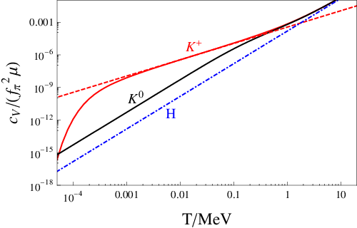
By comparing this expression with Eq. (38) we conclude that the low-temperature contribution of the has the same dependence as the contribution, but that the contribution is always larger by a numerical factor which depends on the zero-temperature kaon mass and chemical potential. We show the full numerical result of the kaon specific heat and its comparison with , , and in the left panel of Fig. 3. We see that there is a significant temperature regime in which is a good approximation to the specific heat, i.e., behaves as as opposed to . The presence of this temperature regime depends on the parameters. Here we have chosen the kaon mass and chemical potential such that this regime is relatively large ( only slightly larger than ). For larger values of , this regime is typically smaller or hardly visible (see right panel of Fig. 3). Note also that our temperature scale extends to very small temperatures in the keV regime. In this regime we expect the small mass of the kaon, which is not present in our formalism, to play a role, see remark below Eq. (23).
The discontinuity at the critical point is small and not visible in the plot. At large temperatures, the specific heat again goes like , however with a different prefactor than at low temperatures. In Table 1 we have listed the low- and high- behavior for the kaon specific heat together with the density and susceptibility, to be computed in Sec. III.2. In the table we also show the behavior for the case of no kaon condensation, i.e., for .
| low | high | ||
|---|---|---|---|
| CFL- | CFL | CFL | |
| kaon specific heat | |||
| kaon density | |||
| kaon susceptibility | |||
So far we have ignored the charged kaons. Due to the electric charge neutrality condition their number density is suppressed at small temperatures [46]. However, in the isospin symmetric case they give rise to an additional Goldstone mode [58, 59, 46] which in principle gives a large contribution to the specific heat. To illustrate this contribution we ignore the neutrality constraint for simplicity and compute the specific heat for a fixed charged kaon chemical potential . For low momenta and exact isospin symmetry , the additional Goldstone mode has a quadratic dispersion, . Consequently, its contribution to the specific heat goes like , just as the contribution from Eq. (39),
| (41) |
We may use the formalism of Ref. [46] to compute the thermal masses in the two-component system of neutral and charged kaons and derive the specific heat analogously to the above one-component system. The numerical result is shown in the right panel of Fig. 3. For this plot we have chosen the kaon masses and chemical potentials such that the isospin symmetry is almost exact. We see that there is a large contribution from the charged kaon mode which disappears for sufficiently small temperatures. This is due to the small isospin symmetry violation in the parameters and hence a small charged kaon energy gap.
Physical case (-dominated) Isospin-symmetric scenario ( and )

III Bulk viscosity in the CFL- phase
We now turn to the main part of the paper where we use the results of the previous sections to compute the bulk viscosity in the CFL- phase.
III.1 Definition of bulk viscosity
The definition of the bulk viscosity and the derivation of its expression in terms of the kaon rate can be found in Ref. [24]. Therefore, here we only briefly summarize the most important relations and the underlying physics. In general, a relativistic superfluid may have more than one bulk viscosity, related to stresses in the superfluid flow with respect to the normal flow [60, 11, 61]. Here we neglect this effect and compute the bulk viscosity related to the normal fluid.
We are interested in a system with volume which undergoes a volume oscillation with amplitude and frequency ,
| (42) |
In the astrophysical setting, the oscillations are local volume oscillations with an (inverse) time scale typically of the order of the rotation frequency of the star which can be as large as . The periodic change in volume induces a change in density. This change in density, in turn, may induce a change in the chemical composition of the matter. In CFL- matter, there will be a change in the strangeness content, described by an induced nonzero , i.e., the equilibrium kaon chemical potential is shifted to the nonequilibrium value . The response of the system is to create (or annihilate) kaons in order to reequilibrate. The dominant processes considered here that change kaon number (and thus strangeness) are
| (43a) | |||
| (43b) | |||
These processes have also been considered in Ref. [24] for the case of uncondensed kaons. If the kaons are condensed there is also a cubic interaction, induced by attaching one leg of the quartic interaction to the condensate, which directly moves strangeness between the condensate and the thermal kaon gas. Here we neglect these processes since they are proportional to the condensate. This is consistent with our 2PI treatment which is only valid for small condensates, i.e. .
The processes (43) induce, in response to the external oscillation , an oscillation in the kaon chemical potential . If the external oscillation and the system’s response are out of phase, there will be dissipation, resulting in a nonzero value of the bulk viscosity. The bulk viscosity is maximized if the external oscillation and the rate of kaon production (annihilation) is on the same time scale. In this sense, bulk viscosity is a resonance phenomenon. In fact, it is the exact analogue of an electric circuit with alternating voltage that responds by an induced alternating current [20].
The definition of the bulk viscosity is
| (44) |
where the dissipated power is given by
| (45) |
The imaginary part of the complex amplitude is given by
| (46) |
where the complex amplitudes , account for the oscillating change in the chemical potentials,
| (47a) | |||||
| (47b) | |||||
Here, and are the quark number density and chemical potential, while and are the corresponding kaon quantities. Note that the effective potential (13) also depends on the quark chemical potential . In particular, the quark density is nonvanishing and there is an induced oscillation also in . This effect, however, is small. In Appendix B we present the general derivation of the bulk viscosity, taking into account the quark density effect. Here we proceed by only keeping the kaon terms. In this case, there is a single differential equation for ,
| (48) |
The left-hand side of this equation simply means that the kaon density is a function of the kaon chemical potential, hence the time dependence of can be expressed in terms of the time dependence of . The right-hand side expresses this change in terms of the volume change (first term) and the kaon rate (second term). The kaon rate is defined as the change in kaon number per time and volume due to the processes (43). For the microscopic definition of see Eq. (65) in Sec. III.3. For sufficiently small we can approximate by
| (49) |
This defines the factor to be positive (for , the system responds by annihilating kaons, hence ; on the other hand, if , the system responds by creating kaons and thus ; in both cases we thus have ). Inserting Eqs. (42), (47a), and (49) into Eq. (48) and inserting the resulting solution for into Eqs. (46), (45), and (44) yields the bulk viscosity
| (50) |
where we have denoted the kaon number susceptibility
| (51) |
In the following we shall evaluate the bulk viscosity (50). To this end, we shall compute the equilibrium density and susceptibility in Sec. III.2, the kaon rate in Sec. III.3, and put the results together in Sec. III.4.
III.2 Kaon density and kaon susceptibility
The kaon density is given by the negative of the derivative of the effective potential (13) with respect to the chemical potential,
| (52) |
Here we have only taken the explicit derivative with respect to . Implicit dependencies through the self-consistent condensate and the kaon mass drop out of the density when we take the value of at the stationary point. Inserting the tree-level potential (8) and the propagators (II.2) and (II.2) yields (see also Ref. [46])
| (53) |
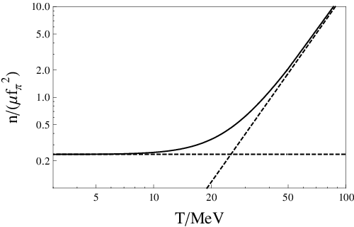
with the integral defined in Eq. (19) and the kaon excitation energy from Eq. (23). At zero temperature, the integral over the Bose distribution function (as well as the integral ) vanishes, and the density is nonzero only because of a nonzero value of ; in other words, all kaons are condensed. Note that the effective coupling , see Eq. (9), depends on the kaon chemical potential. With the zero-temperature value of the condensate we easily obtain the low-temperature limit of the density,
| (54) |
The expansion of this limit for small condensates and the opposite limit for high temperatures are shown Table 1. The two limits are compared with the full numerical result in the left panel of Fig. 4.
The derivation of the susceptibility is more complicated. The susceptibility is the second derivative of the pressure with respect to the chemical potential, and the dependence of and on does not drop out. Hence we have to compute analogously to the specific heat, which is also a second derivative of the pressure. Details of the calculation are presented in Appendix C. The result is
where , , and are given in Eqs. (94) and (95). The zero-temperature limit is obtained from upon approximating the condensate by its zero-temperature value, ,
| (59) |
The high- behavior is dominated by the momentum integral in Eq. (III.2). Table 1 shows both limit cases. The full numerical result for the susceptibility and its comparison to the limit cases is shown in the right panel of Fig. 4. In contrast to the density and the specific heat we observe a strong discontinuity at the critical point.

III.3 Rates of the processes and
The final ingredient to the bulk viscosity (50) is the rate due to the processes (43). To this end, we need the imaginary part of the kaon self-energy given by the diagram in Fig. 5.

This is simply the imaginary part of the one-loop propagator (34) multiplied by the square of the vertex [24], where
| (60) |
with the Fermi coupling and the entries of the CKM matrix , . (Microscopically, the interaction can be understood as the weak process , for details see Ref. [24].) Consequently, we obtain
| (61) |
We can now compute the kaon production rate . In the closed-time path formalism (for calculations in a similar context using this formalism see for instance Refs. [62, 57, 20, 63]) the rate can be written as
| (62) |
Here, the self-energies are given by
| (63a) | |||||
| (63b) | |||||
and the propagators are
| (64a) | |||||
| (64b) | |||||
In these propagators we have introduced chemical nonequilibrium by a nonzero which enters the kaon excitation energy . In the self-consistent mass is determined according to the modified chemical potential. This is necessary since the value of the kaon mass is governed by the strong interaction and thus the mass adjusts itself instantaneously compared to the equilibration time of the weak processes (43). The energy in the -functions of the propagators can be understood from the case without kaon condensation. In this case, we have , and simply cancels, (ignoring the change in the self-consistent mass). In the case with condensation, this cancellation is only partial. Inserting Eqs. (63) and (64) into Eq. (62) yields
| (65) |
From this expression it is clear that corresponds to chemical equilibrium because in this case forward and backward rate cancel each other, and . For small we may approximate
| (66) |
This shows that the sign of the rate is determined by the sign of . For positive the system reacts with annihilating kaons, and , while for negative kaons are created, and . With the approximation (66) we see that, to lowest order in , the rate is
| (67) |
in agreement with Ref. [24]. We shall use Eq. (67) for the numerical evaluation of the rate. Before we turn to the results let us first rewrite the rate into a more instructive form. Inserting the self-energy from Eqs. (30) and (31) into Eq. (65), we obtain
| (68) | |||||
This expression is useful to discuss the separate processes that contribute to the rate. From the structure of the Bose distribution functions (interpreting as an ingoing and as an outgoing particle) we see that the kaon rate is composed of four contributions: the processes and (first and second term, respectively) and the inverse processes and (third and fourth term, respectively). As expected, we see that the kaon-creating processes yield a positive contribution to while the kaon-annihilating processes yield a negative contribution. Furthermore, we conclude that in the CFL- phase (and for infinitesimal ) only the processes are allowed. This can be seen from the dispersion relation in Eq. (23) which implies for . Then, due to the step functions in Eq. (68), the process is excluded. This is of course a direct consequence of energy conservation.
For small temperatures we can derive an analytic expression for the rate in the CFL- phase. The derivation is presented in Appendix D. The result is
| (69) |
where is a complicated dimensionless function of the zero-temperature mass and chemical potential given in Eq. (102). We can simplify this expression by defining
| (70) |
and expanding for small values of , which corresponds to small kaon condensates. This yields
| (71) |
The full evaluation of the rate has to be done numerically; we have checked that the expression (69) is in very good agreement with the full result up to temperatures . The additional approximation (71) is accurate to within 30% for values of .


In the left panel of Fig. 6 we show the numerical result for as a function of the temperature. From Eq. (60) we have ; moreover, we use . We compare the rate in the CFL- phase with the one in the CFL phase. To realize these two cases we choose the kaon chemical potential slightly above and slightly below the kaon mass.
The main features of the two rates are as follows. At very small temperatures, the rate in the CFL- phase is larger than in the CFL phase; parametrically, the former behaves as while the latter is exponentially suppressed. At very large temperatures, the two rates are almost identical. In the intermediate temperature regime however, which is the regime relevant for neutron stars, the rate in the CFL phase is much larger. The reason is a larger phase space for the weak process, as we shall explain in detail in the following.
The kaon width is largest for kaons of momentum such that the internal particle in the kaon self-energy diagram Fig. 5 is closest to being on shell: the and with this momentum both have the same energy, , and the denominator of Eq. (67) is then minimized. From the kaon excitation energies in Eq. (23) we conclude
| (72) |
In the CFL- phase there will be much less phase space associated with the maximum in the kaon width, because it occurs at zero momentum, so one expects the total kaon rate to be lower. Whether the additional phase space in the CFL case is available and has a significant effect on the rate depends on the temperature. For sufficiently large temperatures, , where states well above are thermally populated, the effect of the peak at is negligible. Moreover, for large momenta the kaon dispersion is independent of whether there is a condensate or not; the dispersion then is simply linear, . This is the reason why the two curves in the left panel of Fig. 6 are, at large , almost on top of each other (the small difference in the curves is simply due to the different values of , not because of any qualitative difference between the phases). In other words, besides the values for given in Eq. (72), is also satisfied asymptotically for large (in both CFL- and CFL phases alike). This momentum regime becomes available at large temperatures, and thus the rates become almost identical. For smaller (but not too small) temperatures the peak in the integrand in the CFL phase is responsible for the large kaon rate compared to the CFL- phase. For sufficiently small temperatures, , states around are no longer populated. Therefore, the rate in the CFL- phase, which has its largest contribution from momenta close to zero, becomes larger than the rate in the CFL phase which becomes exponentially suppressed.
III.4 Results for the bulk viscosity
We can now put together the results from the previous subsections to compute the bulk viscosity. We insert the numerical results for the density , see Eq. (53) and left panel of Fig. 4, for the susceptibility , see Eq. (III.2) and right panel of Fig. 4, and for the kaon rate , see Eq. (67) and left panel of Fig. 6, into the expression for the bulk viscosity (50). We shall first analyze the features of the bulk viscosity below the critical temperature and compare the result with the bulk viscosity in the CFL phase. We shall use as a parameter to distinguish between the CFL phase () and the CFL- phase (). Then, we analyze the behavior of the bulk viscosity at the critical point. This of academic rather than physical interest since the critical temperature is likely to exceed temperatures reached in a compact star. Finally, we shall discuss the parameter dependence on and compare the results with the bulk viscosity in other quark matter phases.
III.4.1 CFL- vs. CFL bulk viscosity
We first use the parameters of the rates shown in the left panel of Fig. 6 to compute the corresponding bulk viscosities of the CFL and CFL- phases. The result is shown in the right panel of Fig. 6. We have chosen an oscillation frequency which is typical for a compact star. Let us first discuss the gross features of the result, valid for both CFL and CFL- phases. As explained in Sec. III.1, if the prefactor is held constant, the bulk viscosity becomes maximal if the frequency and the rate of the processes (43) are on the same timescale. More precisely, we have to compare with the effective rate which appears in the bulk viscosity. As a very rough estimate, we read off from Fig. 4 that the susceptibility is of the order of (using ). This means that the kaon rate has to be of the order of to render the effective rate of the order of a frequency in the ms-1 regime. We see from the left panel of Fig. 6 that this is the case for large temperatures, . And indeed we observe that the bulk viscosity has a maximum in this temperature regime. Far below these temperatures we have , and the bulk viscosity can be approximated by . We now discuss the CFL- and CFL results separately in this low temperature regime.
In the CFL- phase, the entire temperature dependence of the low-temperature bulk viscosity is given by the rate because the density and the susceptibility tend to constant values at low . This can also be seen by comparing the two curves in the left and right panels of Fig. 6. With the low-temperature expression for the rate (71) and the values for and from Table 1 we obtain the bulk viscosity in the CFL- phase at small temperatures. To lowest order in , corresponding to small condensates, we find
| (73) |
In the CFL phase without kaon condensation, the rate behaves very differently at small temperatures: it is exponentially suppressed, . The prefactor contributes an additional factor of , . In Fig. 6 we confirm that the bulk viscosity at low in the CFL phase has a different dependence than the kaon rate.
III.4.2 Critical behavior of the bulk viscosity
Next we turn to the behavior of the bulk viscosity at the critical temperature where kaon condensation disappears, and there is a transition from the CFL- phase to CFL. This is probably not relevant to astrophysics, for two reasons. Firstly, one would have to fine tune the kaon mass and chemical potential to bring this critical temperature down to typical compact star temperatures. Secondly, the critical temperature for kaon condensation is of the same order as the critical temperature for the underlying CFL condensate itself [46], so there may really be a transition to unpaired quark matter. However, from the theoretical point of view it might be interesting to compare the critical behavior of the bulk viscosity in the present context with the critical behavior in related systems. For example, the bulk viscosity in a hot quark-gluon plasma has recently been studied [64, 65, 66], and simple models not unlike the one we use for kaons in this paper have been employed to study the behavior at the critical point [67], see also [68].

With the help of Eq. (50) we can make qualitative predictions of the behavior of the bulk viscosity at the critical point. For small values of the frequency, , the viscosity behaves like . Both the density and the rate are continuous at the phase transition, hence the bulk viscosity is continuous too. On the other hand, for large frequencies, , the bulk viscosity behaves like . From Fig. 4 we know that the susceptibility is discontinuous at (and large for temperatures below and close to ). Consequently, we expect the bulk viscosity to be discontinuous too (and small slightly below ). We show the numerical result for the bulk viscosity around the critical point in Fig. 7. The case of an almost continuous behavior as well as the case of a strongly discontinuous behavior is shown (for the latter we have chosen a frequency which is larger than any known compact star rotation rate).
III.4.3 Parameter dependence and comparison to other quark phases
Finally, in Fig. 8, we present the bulk viscosity for several values of the kaon chemical potential and compare the result with the bulk viscosity of unpaired quark matter [17]. As discussed in Sec. II.1, the values of and the kaon mass are poorly known at densities relevant for compact stars. We therefore vary the relevant parameters over ranges of values that are plausible for conditions in a compact star. We fix the kaon mass at and study six values of the effective kaon chemical potential ; for three of them is positive (corresponding to the CFL phase) and for the other three is negative (corresponding to the CFL- phase). We have restricted our plot to temperatures appropriate to compact stars, i.e., we have not shown temperatures larger than .
In the CFL phase, the energy gap for the kaon is , so the thermal population of kaons, and hence the kaon-decay contribution to the bulk viscosity, will be very sensitive to the value of , and will drop rapidly as for . In the CFL- phase, on the other hand, there is always a massless Goldstone kaon, so the bulk viscosity due to kaon decay should be less sensitive to , and should not drop exponentially at low temperatures. These expectations are borne out in Fig. 8. Although the CFL- phase, thanks to its Goldstone mode, has a higher bulk viscosity at very low temperatures, we see that in the range the CFL phase has a larger kaon-decay bulk viscosity than the CFL- phase. This is because of the phase space available at the “resonance” (see the end of Sec. III.3). There is another contribution to the bulk viscosity, from , which starts to become comparable to the contribution from kaon decay at [22].

The bulk viscosity of CFL/CFL- matter is only comparable to that of unpaired quark matter at relatively high temperatures, of order . At lower temperatures the bulk viscosity of CFL/CFL- quark matter is several orders of magnitude smaller. This is the case not only in comparison to the unpaired phase but to all other color-superconducting phases with ungapped fermionic modes—these have bulk viscosities comparable to that of the unpaired phase, and even larger at high temperatures [20]. The only other color-superconducting phase besides the CFL/CFL- phase in which all fermions may be gapped is the color-spin locked phase [36, 39, 69, 70]. For a discussion of its bulk viscosity see Ref. [21].
IV Summary and conclusions
We have computed the bulk viscosity of kaon-condensed CFL quark matter (CFL- phase). Kaon condensation affects the low-energy properties significantly and therefore has a significant effect on thermodynamic and transport properties of color-flavor locked quark matter. In particular, the CFL- phase has a massless bosonic excitation associated with kaon condensation which is absent in the pure CFL phase. In both CFL- and CFL phases, there is also a massless Goldstone mode associated with superfluidity. For most of the thermodynamic properties, the effect of the additional Goldstone mode is important, but rather easy to predict. We have shown this for the specific heat, which acquires a contribution of the kaon mode which, as expected, has the same temperature dependence as the contribution of the superfluid mode. The prefactor of the former, however, is typically larger than that of the latter such that the kaon contribution in fact dominates the specific heat at low temperatures.
The effect of the additional Goldstone mode on the bulk viscosity is more complicated. We have used the results of our earlier work [46] which provides a self-consistent description of the CFL- phase for arbitrary temperatures. Using the resulting thermal kaon mass and excitation energy, we have computed the density and the susceptibility of kaons, both of which are needed for the bulk viscosity. Moreover, we have computed the rate of the processes and , where we denote by both the neutral kaon in the CFL phase and the massless Goldstone mode arising upon kaon condensation in the CFL- phase. These weak processes serve to re-establish chemical (flavor) equilibrium in response to an external volume oscillation, hence giving rise to a nonvanishing bulk viscosity.
At very high temperatures, , the difference in the kaon excitations in the CFL and CFL- phase is negligible. Consequently, in this case the kaon production (and annihilation) rate is almost identical for the two phases. At smaller (but not too small) temperatures, , the masslessness of the Goldstone mode in the CFL- phase suppresses this rate because of a smaller available phase space for the weak process. Since the timescale of the rates in both phases is smaller than the typical oscillation (and rotation) frequency in a compact star, this effect decreases the bulk viscosity of the CFL- phase compared to the CFL phase. Another effect is given through the different susceptibilities. In the condensed system, the susceptibility at low temperatures is much larger than that of the uncondensed system. This effect works in the same direction, further decreasing the bulk viscosity compared to the uncondensed system. For even smaller temperatures, the phase space actually is larger in the CFL- phase and consequently the bulk viscosity is larger too. It is interesting to note that for the neutrino emissivity the effect of kaon condensation is quite different: neutrino emissivity in the CFL- phase is larger than in the CFL phase for all temperatures [71].
We now have a fairly complete understanding of bulk viscosity in color-flavor-locked phases of quark matter. The suppression of the bulk viscosity due to the absence of ungapped fermionic excitations was predicted in Ref. [16]. Subsequent more careful calculations took into account the contribution of the superfluid [22] and kaonic [24] Goldstone modes. With the result of the present paper we have shown that the conclusion already drawn in Ref. [16] is, for temperatures , not changed by the contribution of the Goldstone modes: color-flavor locked quark matter, even in the presence of kaon condensation, has a much lower bulk viscosity than all other known phases of dense quark matter and than nuclear matter. Only at large temperatures, and thus in very young neutron stars, can the contribution of the Goldstone modes render the bulk viscosity comparable to that of unpaired quark matter.
We finally mention that besides the bulk (and shear) viscosity, other properties of color-superconducting quark matter also deserve attention. Its equation of state may be used to put constraints on the mass-radius relation of hybrid stars with a quark matter core and a hadronic mantle. These calculations rely on simple models whose parameters are poorly known in the strong-coupling region of interest. While NJL model calculations, mainly due to their relatively large predicted strange quark mass, tend to find no stable hybrid star with a CFL core [72, 73], other parametrizations of the equation of state allow for hybrid stars with masses compatible with the observations [74]. Other observables that may distinguish between certain phases of color-superconducting quark matter or between quark matter and nuclear matter are for instance the cooling curve of the star or glitches (sudden spin-ups). The corresponding transport properties of color superconductors have already been computed in the literature, see for instance Refs. [75, 57, 63, 76] and Ref. [77] for neutrino emissivity and shear modulus, respectively. It is an interesting and promising task for the future to extend these calculations and compare them with more and better astrophysical data in order to understand matter inside a compact star, and, ultimately, map out the phase diagram of cold and dense quark matter.
Acknowledgements.
The authors acknowledge valuable discussions with M. Huang, C. Manuel, H. Meyer, K. Rajagopal, A. Rebhan, I. Shovkovy, A. Steiner, and M. Tachibana, and support by the U.S. Department of Energy under contracts #DE-FG02-91ER40628, #DE-FG02-05ER41375 (OJI). A.S. ackowledges support by the FWF project P19526.Appendix A Specific heat in the 2PI formalism
Here we derive the expression for the specific heat in the 2PI formalism. We have to take into account that the condensate as well as the full propagator are implicit functions of the temperature (remember that contains the self-consistent thermal mass ). With the definition (35) we thus have to compute
| (74) |
under the contraint that at the stationary point
| (75a) | |||||
| (75b) | |||||
We find
| (76) |
From the constraint (75) we obtain
| (77) |
Inverting the matrix explicitly and inserting the result into Eq. (76) shows that the expressions in parentheses vanish separately, and we are left with
| (78) |
We thus have to apply the differential operator on the explicit derivative of with respect to . From Eq. (22) we find
| (79) |
At the stationary point, the second term in this expression vanishes. This leaves the first term as the result for the entropy density. In order to compute the second derivative, however, we have to keep the second term. By applying the differential operator on this expression, the specific heat can be evaluated in a purely numerical way. For a further analytical evaluation we proceed as follows. In terms of the self-consistent quantities and we can write as (since only depends on the squares and we may take the derivatives with respect to the squares)
| (80) |
The second derivatives of the pressure are straightforwardly obtained from Eq. (79). The derivatives of and with respect to the temperature depend on the stationarity equations. Below the critical temperature, one obtains the derivatives from Eqs. (18a) and (18b). Above the critical temperature, Eq. (18a) is automatically fulfilled and the only equation is Eq. (18b) with set to zero. Consequently, the derivatives assume different functional forms below and above the critical temperature. We find
Now we can insert these expressions and the second derivatives of the pressure obtained from Eq. (79) into Eq. (80) and evaluate the result at the stationary point, i.e., we use Eqs. (18). The result is
| (82) |
With Eq. (81) one then obtains the results below and above the critical temperature. The discontinuity at then is
| (83) |
Appendix B Bulk viscosity with quark number effects
In this appendix we derive the bulk viscosity taking into account the oscillations in the quark chemical potential as given in Eq. (47b). Instead of the simplified single differential equation (48) this yields the two coupled equations
| (84a) | |||||
| (84b) | |||||
We insert the form of the volume oscillation (42) and Eqs. (47) into these differential equations and find the solution
| (85a) | |||||
| (85b) | |||||
where denotes the Jacobian of the two-valued function ,
| (86) |
Inserting Eqs. (85) into the definition of the bulk viscosity yields
| (87) |
This is the general form of the bulk viscosity where the derivatives of the chemical potentials with respect to the densities are obtained by inverting the Jacobian (86). We now assume that the quark chemical potential enters the densities only through the kaon chemical potential, see Eq. (5). This means that we neglect the dependence on through and in Eq. (4). Defining the small dimensionless quantity
| (88) |
we then simply have and
| (89) |
Consequently, Eq. (87) becomes
| (90) |
Neglecting the term proportional to yields the result (50) that we use in the main part of the paper.
Appendix C Number susceptibility in the 2PI formalism
In this appendix we derive an expression for the kaon number susceptibility . Since is given by the second derivative of the pressure (22) with respect to the chemical potential, we can use the same formalism as in Appendix A, where we have computed the second derivative with respect to the temperature. Consequently, with the same arguments as in Appendix A (cf. Eq. (80))
| (91) |
We determine the derivatives of and with respect to from the stationarity equations (18). They are
where we have abbreviated , . Note that the effective coupling constant depends on the kaon chemical potential , see Eq. (9). Next, we compute the second derivatives of the pressure appearing in Eq. (91) with the help of Eq. (22). Putting everything together we obtain the susceptibility,
where the zero-temperature part is
| (94) |
and where
| (95a) | |||||
| (95b) | |||||
Appendix D Low-temperature result for the kaon rate
In this appendix we derive Eq. (69), the low-temperature expression for the kaon rate in the presence of a kaon condensate. To this end, we first compute the low-temperature result for the imaginary part of the retarded self-energy. Below the critical temperature we have for all (see Eq. (23)) and thus we have
| (96) |
For small temperatures only small momenta are relevant, and we can use the small-momentum approximation of the excitation energy given in Eq. (24). Moreover, since we consider temperatures well below the critical temperature, the quadratic part of the kaon dispersion is negligible. Therefore, , with the abbreviation
| (97) |
Here we have used the zero-temperature result for the self-consistent mass . With the new integration variable we have approximately
| (98) |
Note that and are of the same order. Therefore we cannot simply drop the terms in the square brackets that are of higher order in . We rather have to keep all the terms. The integration can be done exactly and we obtain
| (99) |
where, for the sake of brevity, we have used . We can now insert the result into the rate (67). In the denominator of the integrand we neglect the term . No further approximation is then required to obtain the final result. We make use of
| (100) |
where is the generalized zeta function, and where we need the cases . Then we arrive at
| (101) |
with the dimensionless function
| (102) | |||||
Inserting the expression for from Eq. (97) into Eq. (101) yields the final result given in the main text, see Eq. (69).
References
- [1] M. G. Alford, A. Schmitt, K. Rajagopal, and T. Schafer (2007a), eprint arXiv:0709.4635 [hep-ph].
- [2] D. J. Gross and F. Wilczek, Phys. Rev. Lett. 30, 1343 (1973).
- [3] H. D. Politzer, Phys. Rev. Lett. 30, 1346 (1973).
- [4] N. Andersson, Astrophys. J. 502, 708 (1998), eprint gr-qc/9706075.
- [5] L. Lindblom (2000), eprint astro-ph/0101136.
- [6] B. J. Owen et al., Phys. Rev. D58, 084020 (1998), eprint gr-qc/9804044.
- [7] P. Haensel, K. P. Levenfish, and D. G. Yakovlev, Astron. Astrophys. 357, 1157 (2000), eprint astro-ph/0004183.
- [8] P. Haensel, K. P. Levenfish, and D. G. Yakovlev (2001a), eprint astro-ph/0103290.
- [9] N. Andersson, G. L. Comer, and K. Glampedakis, Nucl. Phys. A763, 212 (2005), eprint astro-ph/0411748.
- [10] D. Chatterjee and D. Bandyopadhyay, Phys. Rev. D75, 123006 (2007a), eprint astro-ph/0702259.
- [11] M. E. Gusakov, Phys. Rev. D76, 083001 (2007), eprint 0704.1071.
- [12] D. Chatterjee and D. Bandyopadhyay (2007b), eprint arXiv:0712.3171 [astro-ph].
- [13] D. Chatterjee and D. Bandyopadhyay (2007c), eprint arXiv:0712.4347 [astro-ph].
- [14] L. Lindblom and B. J. Owen, Phys. Rev. D65, 063006 (2002), eprint astro-ph/0110558.
- [15] P. Haensel, K. P. Levenfish, and D. G. Yakovlev (2001b), eprint astro-ph/0110575.
- [16] J. Madsen, Phys. Rev. Lett. 85, 10 (2000), eprint astro-ph/9912418.
- [17] J. Madsen, Phys. Rev. D46, 3290 (1992).
- [18] B. A. Sa’d, I. A. Shovkovy, and D. H. Rischke, Phys. Rev. D75, 125004 (2007a), eprint astro-ph/0703016.
- [19] C. Manuel, A. Dobado, and F. J. Llanes-Estrada, JHEP 09, 076 (2005), eprint hep-ph/0406058.
- [20] M. G. Alford and A. Schmitt, J. Phys. G34, 67 (2007), eprint nucl-th/0608019.
- [21] B. A. Sa’d, I. A. Shovkovy, and D. H. Rischke, Phys. Rev. D75, 065016 (2007b), eprint astro-ph/0607643.
- [22] C. Manuel and F. Llanes-Estrada, JCAP 0708, 001 (2007), eprint arXiv:0705.3909 [hep-ph].
- [23] H. Dong, N. Su, and Q. Wang, J. Phys. G34, S643 (2007), eprint astro-ph/0702181.
- [24] M. G. Alford, M. Braby, S. Reddy, and T. Schäfer, Phys. Rev. C75, 055209 (2007b), eprint nucl-th/0701067.
- [25] M. G. Alford, K. Rajagopal, and F. Wilczek, Nucl. Phys. B537, 443 (1999), eprint hep-ph/9804403.
- [26] D. T. Son and M. A. Stephanov, Phys. Rev. D61, 074012 (2000a), eprint hep-ph/9910491.
- [27] P. F. Bedaque and T. Schäfer, Nucl. Phys. A697, 802 (2002), eprint hep-ph/0105150.
- [28] D. B. Kaplan and S. Reddy, Phys. Rev. D65, 054042 (2002), eprint hep-ph/0107265.
- [29] M. M. Forbes, Phys. Rev. D72, 094032 (2005), eprint hep-ph/0411001.
- [30] M. Buballa, Phys. Lett. B609, 57 (2005), eprint hep-ph/0410397.
- [31] H. J. Warringa (2006), eprint hep-ph/0606063.
- [32] M. Ruggieri, JHEP 07, 031 (2007), eprint 0705.2974.
- [33] D. Ebert, K. G. Klimenko, and V. L. Yudichev, Eur. Phys. J. C53, 65 (2008), eprint arXiv:0705.2666 [hep-ph].
- [34] V. Kleinhaus, M. Buballa, D. Nickel, and M. Oertel, Phys. Rev. D76, 074024 (2007), eprint 0707.0632.
- [35] K. Rajagopal and A. Schmitt, Phys. Rev. D73, 045003 (2006), eprint hep-ph/0512043.
- [36] T. Schäfer, Phys. Rev. D62, 094007 (2000), eprint hep-ph/0006034.
- [37] M. G. Alford, J. A. Bowers, J. M. Cheyne, and G. A. Cowan, Phys. Rev. D67, 054018 (2003), eprint hep-ph/0210106.
- [38] A. Schmitt, Q. Wang, and D. H. Rischke, Phys. Rev. D66, 114010 (2002), eprint nucl-th/0209050.
- [39] A. Schmitt, Phys. Rev. D71, 054016 (2005), eprint nucl-th/0412033.
- [40] M. G. Alford, J. A. Bowers, and K. Rajagopal, Phys. Rev. D63, 074016 (2001), eprint hep-ph/0008208.
- [41] K. Rajagopal and R. Sharma, J. Phys. G32, S483 (2006), eprint hep-ph/0606066.
- [42] M. Mannarelli, K. Rajagopal, and R. Sharma, Phys. Rev. D73, 114012 (2006), eprint hep-ph/0603076.
- [43] A. Kryjevski, Phys. Rev. D77, 014018 (2008), eprint hep-ph/0508180.
- [44] T. Schäfer, Phys. Rev. Lett. 96, 012305 (2006), eprint hep-ph/0508190.
- [45] A. Gerhold, T. Schäfer, and A. Kryjevski, Phys. Rev. D75, 054012 (2007), eprint hep-ph/0612181.
- [46] M. G. Alford, M. Braby, and A. Schmitt, J. Phys. G35, 025002 (2008), eprint arXiv:0707.2389 [nucl-th].
- [47] J. M. Luttinger and J. C. Ward, Phys. Rev. 118, 1417 (1960).
- [48] G. Baym, Phys. Rev. 127, 1391 (1962).
- [49] J. M. Cornwall, R. Jackiw, and E. Tomboulis, Phys. Rev. D10, 2428 (1974).
- [50] J. T. Lenaghan and D. H. Rischke, J. Phys. G26, 431 (2000), eprint nucl-th/9901049.
- [51] D. Roder, J. Ruppert, and D. H. Rischke, Phys. Rev. D68, 016003 (2003), eprint nucl-th/0301085.
- [52] J. O. Andersen, Phys. Rev. D75, 065011 (2007), eprint hep-ph/0609020.
- [53] D. T. Son (2001), eprint hep-ph/0108260.
- [54] D. T. Son and M. A. Stephanov, Phys. Rev. D62, 059902 (2000b), eprint hep-ph/0004095.
- [55] D. T. Son (2002), eprint hep-ph/0204199.
- [56] T. Schäfer and K. Schwenzer, Phys. Rev. D70, 114037 (2004), eprint astro-ph/0410395.
- [57] A. Schmitt, I. A. Shovkovy, and Q. Wang, Phys. Rev. D73, 034012 (2006), eprint hep-ph/0510347.
- [58] V. A. Miransky and I. A. Shovkovy, Phys. Rev. Lett. 88, 111601 (2002), eprint hep-ph/0108178.
- [59] T. Schäfer, D. T. Son, M. A. Stephanov, D. Toublan, and J. J. M. Verbaarschot, Phys. Lett. B522, 67 (2001), eprint hep-ph/0108210.
- [60] N. Andersson and G. L. Comer, Living Rev. Rel. 10, 1 (2005), eprint gr-qc/0605010.
- [61] M. Mannarelli and C. Manuel, Phys. Rev. D77, 103014 (2008), eprint 0802.0321.
- [62] M. Schonhofen, M. Cubero, B. L. Friman, W. Norenberg, and G. Wolf, Nucl. Phys. A572, 112 (1994).
- [63] P. Jaikumar, C. D. Roberts, and A. Sedrakian, Phys. Rev. C73, 042801 (2006), eprint nucl-th/0509093.
- [64] P. Arnold, C. Dogan, and G. D. Moore, Phys. Rev. D74, 085021 (2006), eprint hep-ph/0608012.
- [65] H. B. Meyer, Phys. Rev. Lett. 100, 162001 (2008), eprint 0710.3717.
- [66] F. Karsch, D. Kharzeev, and K. Tuchin, Phys. Lett. B663, 217 (2008), eprint 0711.0914.
- [67] J.-W. Chen, M. Huang, Y.-H. Li, E. Nakano, and D.-L. Yang (2007), eprint 0709.3434.
- [68] J.-W. Chen and J. Wang (2007), eprint 0711.4824.
- [69] F. Marhauser, D. Nickel, M. Buballa, and J. Wambach, Phys. Rev. D75, 054022 (2007), eprint hep-ph/0612027.
- [70] D. N. Aguilera, D. Blaschke, M. Buballa, and V. L. Yudichev, Phys. Rev. D72, 034008 (2005), eprint hep-ph/0503288.
- [71] S. Reddy, M. Sadzikowski, and M. Tachibana, Phys. Rev. D68, 053010 (2003), eprint nucl-th/0306015.
- [72] M. Baldo et al., Phys. Lett. B562, 153 (2003), eprint nucl-th/0212096.
- [73] T. Klahn et al., Phys. Lett. B654, 170 (2007), eprint nucl-th/0609067.
- [74] M. G. Alford, M. Braby, M. W. Paris, and S. Reddy, Astrophys. J. 629, 969 (2005), eprint nucl-th/0411016.
- [75] P. Jaikumar, M. Prakash, and T. Schäfer, Phys. Rev. D66, 063003 (2002), eprint astro-ph/0203088.
- [76] R. Anglani, G. Nardulli, M. Ruggieri, and M. Mannarelli, Phys. Rev. D74, 074005 (2006), eprint hep-ph/0607341.
- [77] M. Mannarelli, K. Rajagopal, and R. Sharma, Phys. Rev. D76, 074026 (2007), eprint hep-ph/0702021.