Effective Interacting Hamiltonian and Pairing Symmetry of LaOFeAs

The recent discovery of the new family of iron based high-$T_{c}$ superconductors [1, 2, 3, 4, 5] has attracted intensive experimental [6, 7] and theoretical interests. Although at the current stage little is known for its microscopic origin, theory has made great advances in understanding the electronic structures [8, 11, 9, 10]. In particular, a number of pairing mechanisms and pairing symmetries have been proposed [8, 12, 9, 13, 14, 15, 16, 17, 18]. In most of these studies, the microscopic Hamiltonian adopted is deterministic for the outcome of theory. It is thus desirable to know the general form of the interacting Hamiltonian allowed by the symmetry of the system, upon which the possible pairing states can be systematically analyzed.

In this paper, we establish the effective interacting Hamiltonian for LaOFeAs system based on the general symmetry consideration. The peculiar symmetry property of electron states near $M$-point yields unusual form of electron-electron ($e$-$e$) interaction. Based on the general effective Hamiltonian, we determine all the possible pairing states allowed by the symmetry. The stability of these pairing states against the band energy splitting and the on-site Coulomb repulsion is discussed. The analysis is general enough to be useful for other systems with the similar electronic structure.

Structure and symmetry. The structure of LaOFeAs consists of the alternating layers of FeAs and LaO planes. The first principles calculations reveal the dominant role of the two-dimensional FeAs planes in electron conduction [8, 11, 9]. Fig. 1 shows the schematic structure of the FeAs plane. The full symmetry group for the system is of $P4/nmm$ [19, 20]. For our purpose, it is sufficient to consider its symmorphic subgroup $P\bar{4}2m$, which is a semi-direct-product of the point group $D_{2d}$ and the lattice translational group. Figure 1 shows the symmetry axes of the eight symmetry operations of $D_{2d}$. The point group has four one-dimensional irreducible representations: $A_{1}$ ($x^{2}+y^{2}$), $A_{2}$ ($xy(x^{2}-y^{2})$), $B_{1}$ ($x^{2}-y^{2}$), $B_{2}$ ($xy$), and a two-dimensional representation $E$ ($(xz,yz)$).

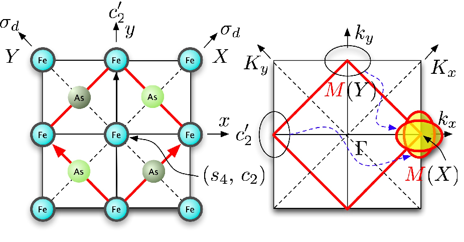
The most notable feature of LaOFeAs system is its multi-orbit nature. The Bloch bands form five small Fermi pockets: three hole pockets at $\Gamma$-point, and two electron pockets at $M$-point. It was suggested that the hole pockets shrink and disappear upon doping, leaving the two electron pockets responsible for the superconductivity [8]. The two electron pockets are of Fe-$d$ orbit origin, and the Bloch states at the $M$-point are essentially $d_{xz}$ and $d_{yz}$. Departing from the $M$-point, these states strongly hybridize with $d_{xy}$ orbit, giving rise to the two elliptically shaped Fermi pockets ¹¹ 1 Due to the strong hybridization, a minimal model to describe the band structure near $M$-point should include at least $d_{xz}$, $d_{yz}$ and $d_{xy}$ orbits [16]..

The electron states near $M$-point have peculiar symmetry property. The two degenerated Bloch states at $M$-point span the subspace for the two-dimensional irreducible representation $E$ of $D_{2d}$. Departing from the $M$-point, the Bloch states $\varphi_{i}(\bm{k},\bm{r})$ ($i=1,2$) of the two bands will be transformed by:

where $\hat{\alpha}\in D_{2d}$ is a symmetry operation, and $D_{ij}^{E}(\alpha)$ is the two-dimensional irreducible representation matrix for $(xz,yz)$. The transformation property can be established by generalizing the usual symmetry argument for Bloch wave-functions with the proper assignment of the band index to the two states at each $\bm{k}$ point, so that the resulting wave functions are continuous functions of $\bm{k}$. Note that Eq. (1) is possible because of the presence of a generalized translational symmetry: the system is invariant under the transformations $T_{x}P_{z}$ and $T_{y}P_{z}$, where $T_{x}$ ($T_{y}$) is the translation along $x$ ($y$) direction by the Fe-Fe distance and $P_{z}$ is the reflection $z\rightarrow-z$ [16]. With the symmetry, one can define a reduced $1\times 1$ primitive cell containing only one Fe atom, and the corresponding extended Brillouin zone, as shown in Fig. 1. The two overlapping Fermi pockets at $M$-point in the real Brillouin zone actually originate from the Fermi pockets located at the two non-equivalent points $X$ and $Y$ of the extended Brillouin zone. Without such a symmetry, the hybridization between different $d$-orbits would re-organize them into two separated Fermi pockets that transform within themselves, instead of the two-dimensional representation shown in Eq. (1). Note that the presence of the generalized translational symmetry does not prohibit interband coupling through $e$-$e$ interaction.

Effective electron-electron interaction. Equation (1) is one of the peculiarities of LaOFeAs system. It is interesting to see how the unique electron structure has effect on the $e$-$e$ interaction. We thus focus on the interaction amongst the two electron pockets, which can be written as:

where $a_{is}^{\dagger}(\bm{k})$ and $a_{is}(\bm{k})$ are the creation and annihilation operators for band $i=1,2$ and spin index $s=\uparrow\downarrow$. We only consider $e$-$e$ interaction relevant to the superconductivity between a pair of electrons with the zero total momentum. The $e$-$e$ interaction should be interpreted as an effective one, including contributions not only from the direct Coulomb interaction, but also from the effective interaction mediated by other degrees of freedom such as phonon, or the renormalization effect due to the projection of the high-energy sectors.

Next we explicitly construct the general interacting Hamiltonian invariant under the symmetry operations. From Eq. (1), it is easy to see that the annihilation operator $a_{i}(\bm{k})$ transforms by $\hat{\alpha}a_{i}(\bm{k})\hat{\alpha}^{-1}=\sum_{j}a_{j}(\hat{\alpha}^{-1}\bm{k})D_{ji}^{E}(\alpha)$, here we ignore the spin indexes for the moment. As a result, the transformations of $a_{i_{1}}^{\dagger}(\bm{k})a_{i_{2}}^{\dagger}(-\bm{k})a_{i_{3}}(-\bm{k}^{\prime})a_{i_{4}}(\bm{k}^{\prime})$ under the symmetry operations belong to the direct-product representation $E\times E\times E\times E$, which can be decomposed to the one-dimensional irreducible representations $4A_{1}\oplus 4A_{2}\oplus 4B_{1}\oplus 4B_{2}$.

The decomposition can be explicitly constructed by the following procedures. First, the two-particle annihilation operator $a_{i}(-\bm{k})a_{j}(\bm{k})$ can be organized to different orbital pairing channels: $\Psi_{0}(\bm{k})\equiv a_{i}(-\bm{k})\tau_{ij}^{0}a_{i}(\bm{k})\sim A_{1}$, $\Psi_{1}(\bm{k})\equiv a_{i}(-\bm{k})\tau_{ij}^{1}a_{j}(\bm{k})\sim B_{2}$, $\Psi_{2}(\bm{k})\equiv a_{i}(-\bm{k})\tau_{ij}^{2}a_{j}(\bm{k})\sim A_{2}$, $\Psi_{3}(\bm{k})\equiv a_{i}(-\bm{k})\tau_{ij}^{3}a_{j}(\bm{k})\sim B_{1}$, where $\tau^{\alpha}$ ($\alpha=1,2,3)$ are the Pauli-matrices, and $\tau^{0}$ is the unity matrix [20]. The symbol $\sim$ indicates the transformation property of the operators. For instance, $\Psi_{0}(\bm{k})\sim A_{1}$ means $\hat{\alpha}\Psi_{0}(\bm{k})\hat{\alpha}^{-1}=D^{A_{1}}(\alpha)\Psi_{0}(\hat{\alpha}^{-1}\bm{k})$, where $D^{A_{1}}(\alpha)$ is the transformation coefficient of the irreducible representation $A_{1}$. Using these bases, the effective $e$-$e$ interaction can be written as:

where $\Psi(\bm{k})\equiv[\Psi_{0},\Psi_{1},\Psi_{2},\Psi_{3}]^{T}$, and all the matrix elements $v_{ij}$ are functions of $(\bm{k},\bm{k}^{\prime})$, and have symmetry $v_{ij}(\bm{k},\bm{k}^{\prime})=v_{ji}^{*}(\bm{k}^{\prime},\bm{k})$. To make the Hamiltonian invariant under the point group operations, $v_{ij}(\bm{k})$ must have certain transformation property. For instance, $\Psi_{1}^{\dagger}(\bm{k})\Psi_{2}(\bm{k}^{\prime})\sim B_{2}\times A_{2}=B_{1}$, i.e., $\hat{\alpha}[\Psi_{1}^{\dagger}(\bm{k})\Psi_{2}(\bm{k}^{\prime})]\hat{\alpha}^{-1}=D^{B_{1}}(\alpha)\Psi_{1}^{\dagger}(\hat{\alpha}^{-1}\bm{k})\Psi_{2}(\hat{\alpha}^{-1}\bm{k}^{\prime})$. To have an invariant partial Hamiltonian $\sum_{\bm{k}\bm{k}^{\prime}}v_{12}(\bm{k},\bm{k}^{\prime})\Psi_{1}^{\dagger}(\bm{k})\Psi_{2}(\bm{k}^{\prime})$, $v_{12}$ must have $v_{12}(\hat{\alpha}^{-1}\bm{k},\hat{\alpha}^{-1}\bm{k}^{\prime})=D^{B_{1}}(\alpha)v_{12}(\bm{k},\bm{k}^{\prime})$, i.e., $v_{12}\sim B_{1}$. Following the same procedure, the symmetry properties of all matrix elements can be determined. They are indicated by the superscripts of $v_{ij}$ in Eq. (3).

To incorporate the spin indexes into the effective interaction, we generalize the pair annihilation operators $\Psi_{\alpha}(\bm{k})\rightarrow\Psi_{\alpha,a}(\bm{k})\equiv a_{is}(-\bm{k})\tau_{ij}^{\alpha}\tau_{ss^{\prime}}^{a}a_{js^{\prime}}(\bm{k})$, where $a$ denotes the spin pairing channel. When the spin-orbit coupling is negligible, the effective $e$-$e$ interaction has the form [21]:

where $\Psi_{,a}(\bm{k})\equiv[\Psi_{0,a},\Psi_{1,a},\Psi_{2,a},\Psi_{3,a}]^{T}$, and the matrices $V^{(s)}(\bm{k},\bm{k}^{\prime})$ and $V^{(t)}(\bm{k},\bm{k}^{\prime})$ denote the effective $e$-$e$ interactions in the spin-singlet $(s)$ and triplet $(t)$ channels, respectively. Both matrices have the same structure as the one presented in Eq. (3). Pauli exclusion principle imposes the further constraints onto the matrix elements: $v_{\alpha\beta}^{(s)}(-\bm{k},\bm{k}^{\prime})=g(\alpha)v_{\alpha\beta}^{(s)}(\bm{k},\bm{k}^{\prime})$, $v_{\alpha\beta}^{(s)}(\bm{k},-\bm{k}^{\prime})=g(\beta)v_{\alpha\beta}^{(s)}(\bm{k},\bm{k}^{\prime})$, and $v_{\alpha\beta}^{(t)}(-\bm{k},\bm{k}^{\prime})=-g(\alpha)v_{\alpha\beta}^{(t)}(\bm{k},\bm{k}^{\prime})$, $v_{\alpha\beta}^{(t)}(\bm{k},-\bm{k}^{\prime})=-g(\beta)v_{\alpha\beta}^{(t)}(\bm{k},\bm{k}^{\prime})$, where $g(\alpha)=-1$ ($1$) for $\alpha=2$ ($\neq 2$). The matrix elements $v_{\alpha\beta}(\bm{k},\bm{k}^{\prime})$ can be further expanded as:

where $f_{n}^{R}(\bm{k})$ denotes a complete set of functions that transform by the irreducible representation $R$. The summation should be run through all the possible combinations of $R_{1}$ and $R_{2}$ which yield $R\in R_{1}\times R_{2}$. For instance, for $v_{03}^{B_{1}}$, there are five possible combinations, $A_{1}\times B_{1}$, $B_{1}\times A_{1}$, $B_{2}\times A_{2}$, $A_{2}\times B_{2}$, $E\times E$, based on the product rules of the group.

To be more explicit, we construct an expression using only the lowest order polynomials for each irreducible representation: $s\sim 1\sim A_{1}$, $g\sim k_{x}k_{y}(k_{x}^{2}-k_{y}^{2})\sim A_{2}$, $d_{x^{2}-y^{2}}\sim k_{x}^{2}-k_{y}^{2}\sim B_{1}$, $d_{xy}\sim k_{x}k_{y}\sim B_{2}$, $[p_{x},p_{y}]\sim[k_{x},k_{y}]\sim E$. Such an expression contains the full information of symmetry. It could also be a good approximation for LaOFeAs system since all its Fermi pockets are small, and the higher ($n$-th) order contributions are scaled by $(k_{F}a)^{n}$, where $a$ is the scattering length of the effective interaction, and $k_{F}$ is the Fermi wave vector. The explicit form of $v_{\alpha\beta}^{(s)}(\bm{k},\bm{k}^{\prime})$ reads:

Similarly, the explicit expression for $v_{\alpha\beta}^{(t)}$ reads:

Possible pairing symmetries. Equations (4)–(17) provide the basis for deducing the possible pairing symmetries. Basically, the interacting Hamiltonian Eq. (4) describes how the electron pairs in different orbital and spin pairing channels are coupled, while Eq. (5) (or (6)–(17)) dictates the coupling between the different momentum pairing symmetries. The pairing instability of the system can be determined by considering a Cooper pair out of the Fermi sea. The Cooper equation reads ²² 2 The equation is actually a linearized BCS gap equation. It is the exact gap equation at the limit of the vanishing gap. ,

where $h_{\alpha\beta}(\bm{k})$ is the kinetic energy of the Cooper pair, and has the non-vanishing elements: $h_{00}(\bm{k})=h_{33}(\bm{k})=|\xi_{1}(\bm{k})|+|\xi_{2}(\bm{k})|$, $h_{11}(\bm{k})=h_{22}(\bm{k})=|\xi_{1}(\bm{k})+\xi_{2}(\bm{k})|$, $h_{03}(\bm{k})=h_{30}(\bm{k})=|\xi_{1}(\bm{k})|-|\xi_{2}(\bm{k})|$, where $\xi_{i}(\bm{k})=\epsilon_{i}(\bm{k})-\mu$ is the single electron band energy relative to the Fermi surface. Note that the interband Cooper pairs cannot exist in the non-overlapping areas of the two Fermi pockets, which are excluded from contributing the interband pairing potential by the measure $w_{\beta}(\bm{k)}$: $w_{0}(\bm{k})=w_{3}(\bm{k})=1$, $w_{1}(\bm{k})=w_{2}(\bm{k})=\theta(\xi_{1}(\bm{k})\xi_{2}(\bm{k}))$, where $\theta(x)$ is the Heaviside function. A bounding state solution of the equation signifies the instability of the normal Fermi liquid, and the resulting superconducting state will have the order parameter $\Delta_{ij,ss^{\prime}}(\bm{k})\sim\tau_{ij}^{\alpha}\tau_{ss^{\prime}}^{a}|\xi_{i}(\bm{k})+\xi_{j}(\bm{k})|\psi_{\alpha,a}(\bm{k})$, approximately.

It is easy to see both $h_{\alpha\beta}$ and $w_{\beta}(\bm{k})$ do not change the symmetry characteristics of Eq. (18) from the one dictated by $v_{\alpha\beta}^{(a)}$. It is thus straightforward to use Eq. (6)–(17) to determine the possible pairing states of the system. It can be readily observed that the pairing states must have the definite parities in exchanging spin/orbit/momentum indexes, as the states with the different parities do not mix. A closer analysis reveals the particular way of mixing between the different pairing symmetries and the orbital pairing channels. For instance, in the spin singlet channel, an $s$-wave component in orbital pairing channel $0$ ($\psi_{0}\sim s$) will induce $\psi_{1}\sim d_{xy}$ (by $v_{01}^{(s)}$) and $\psi_{3}\sim d_{x^{2}-y^{2}}$ (by $v_{03}^{(s)}$). These states form a closed subspace for an eigenstate of Eq. (18). The corresponding superconductivity order parameter has the form [18]:

The similar analyses can be carried out for all other possible combinations. A complete list of all possible pairing states is presented in Table 1.

More physical considerations may further reduce the list of candidates. One of the most important factors is the band energy splitting $\xi_{1}(\bm{k})-\xi_{2}(\bm{k})$, which acts like a “Zeeman” field and will suppress the interband pairings. Its adverse effects to the different interband pairing states have the relative strengths $d_{x^{2}-y^{2}}>s\approx p\approx g>d_{xy}$. The strong band splitting tends to suppress the pure interband pairing states (5) and (7)–(10), although the state (9) may be more robust than the others in the group. On the other hand, those states mixing the interband and intraband pairings, i.e., the states (1)–(4) and (6), may not be as sensitive, as long as the pairing is dominated by the intraband attractive interaction. Another potential factor is the strong on-site Coulomb repulsion, which would suppress $s$-wave components in states (1)–(3) and (7). As a result, the states (1)–(3) will be dominated by the $d$-wave pairing symmetries. Finally, the smallness of the Fermi pockets in LaOFeAs system may also have implications on the possible pairing forms: the screening of the bare $e$-$e$ interaction by the Fermi gas of small $k_{F}$ will render the effective interaction spatially extended. It is thus unlikely for LaOFeAs system to form spatially localized bond-like-pairings, as that happens in high-$T_{c}$ cuprates [20]. Moreover, in the limit of weak coupling ($k_{F}a\ll 1$), one may expect that the attractive $e$-$e$ interaction in the $p$-wave channel, if presents, would be stronger than that in the $d$-wave channels. Note that in many microscopic models, the $p$-wave channel is absent, due to the improper adoption of a two-orbit model for describing the band structure near the $M$-point [16], while the symmetry argument clearly suggests its presence. The possibility of $p$-wave pairing state (i.e., the state (6)) has been demonstrated in Ref. [16], using a microscopic model including three $d$-orbits and on-site Hund’s coupling.

In summary, we have constructed the general effective interacting Hamiltonian conforming to the peculiar symmetry of LaOFeAs system. A complete list of the possible pairing states is also determined. The general effective Hamiltonian can act as a maximal model, from which the minimal model can be constructed for a given pairing state. This is useful since the peculiar symmetry property of the electronic state may render the first-sight intuitions misleading. The ten pairing states put strong constraints to the possible forms of superconductivity, and could act as the consistency check for the proposed pairing symmetries. Finally, our approach is completely general. The result presented here would be useful for other systems with the similar electronic structure.

I thank Xi Dai for useful discussion on the band structure. This work is supported by NSF of China No. 10734110, 10604063 and Ministry of Science and Technology of China under 973 program No. 2006CB921304.

References

- [1] Y. Kamihara, T. Watanabe, M. Hirano, and H. Hosono, J. Am. Chem. Soc. 130, 3296 (2008).
- [2] X. H. Chen, T. Wu, G. Wu, R. H. Liu, H. Chen, and D. F. Fang (2008), eprint arXiv:0803.3603.
- [3] H.-H. Wen, G. Mu, L. Fang, H. Yang, and X. Zhu, Europhys. Lett. 82, 17009 (2008).
- [4] Z.-A. Ren, W. Lu, J. Yang, W. Yi, X.-L. Shen, Z.-C. Li, G.-C. Che, X.-L. Dong, L.-L. Sun, F. Zhou, et al. (2008), eprint arXiv:0804.2053.
- [5] H. Takahashi, K. Igawa, K. Arii, Y. Kamihara, M. Hirano, and H. Hosono, Nature 453, 376 (2008).
- [6] C. de la Cruz, Q. Huang, J. W. Lynn, J. Li, W. Ratcliff, J. L. Zarestky, H. A. Mook, G. F. Chen, J. L. Luo, N. L. Wang, et al. (2008), eprint arXiv:0804.0795.
- [7] J. Dong, H. J. Zhang, G. Xu, Z. Li, G. Li, W. Z. Hu, D. Wu, G. F. Chen, X. Dai, J. L. Luo, et al. (2008), eprint arXiv:0803.3426.
- [8] D. J. Singh and M. H. Du (2008), eprint arXiv:0803.0429.
- [9] K. Kuroki, S. Onari, R. Arita, H. Usui, Y. Tanaka, H. Kontani, and H. Aoki (2008), eprint arXiv:0803.3325.
- [10] K. Haule, J. H. Shim, and G. Kotliar, Phys. Rev. Lett. 100, 226402 (2008).
- [11] H.-J. Zhang, G. Xu, X. Dai, and Z. Fang (2008), eprint arXiv:0803.4487.
- [12] X. Dai, Z. Fang, Y. Zhou, and F. chun Zhang (2008), eprint arXiv:0803.3982.
- [13] Q. Han, Y. Chen, and Z. D. Wang (2008), eprint arXiv:0803.4346.
- [14] X.-L. Qi, S. Raghu, C.-X. Liu, D. J. Scalapino, and S.-C. Zhang (2008), eprint 0804.4332.
- [15] J. Li and Y. Wang, Chin. Phys. Lett. 25,, No.62232 (2008), eprint arXiv:0805.0644.
- [16] P. A. Lee and X.-G. Wen (2008), eprint arXiv:0804.1739.
- [17] Z.-Y. Weng (2008), eprint arXiv:0804.3228.
- [18] K. Seo, B. A. Bernevig, and J. Hu (2008), eprint arXiv:0805.2958.
- [19] Z.-H. Wang, H. Tang, Z. Fang, and X. Dai (2008), eprint arXiv:0805.0736.
- [20] Y. Wan and Q.-H. Wang (2008), eprint arXiv:0805.0923.
- [21] S. Nakajima, Prog. Theor. Phys. 50, 1101 (1973).