Holographic Double Diffractive Scattering
Abstract:
The holographic description of Pomeron exchange in a strongly-coupled gauge theory with an AdS dual is extended to the case of two to three scattering. We study the production event of a central particle via hadron-hadron scattering in the double Regge kinematic regime of large center-of-momentum energy and fixed momentum transfer. The computation reduces to the overlap of a holographic wave function for the central particle with a source function for the Pomerons. The formalism is applied to scalar glueball production and the resulting amplitude is studied in various kinematic limits.
Keywords:
AdS-CFT Correspondence, Phenomenological Models1 Introduction
Regge phenomena have been studied, both in experiments and in theoretical contexts, for several decades. Experiments investigating hadron scattering, and associated theoretical attempts to understand the data, led in the 1960s to a number of important developments that continue to play a role in current research. The general Regge approach to writing amplitudes as complex-valued functions of Mandelstam variables, and investigating them using Mellin transforms, had some general success in characterizing observed amplitudes that appeared at the time to be inconsistent with quantum field theory. The development of “dual resonance” models that captured various features of scattering amplitudes, including - channel duality, towers of resonances lying on Regge trajectories for , and near-forward scattering amplitudes proportional to for , were the first steps along the road to a consistent string theory. Of course, hadronic scattering experiments and standard string theory diverged in large-angle scattering (where the amplitudes for the former fall as powers of , while those of the latter fall exponentially) and in deep inelastic scattering (where Bjorken scaling suggested hard, weakly-interacting substructure). The theory of QCD supplanted string theory as the leading model for strong interactions, and its success is spectacular. Further, it was soon learned that consistent string theories needed to be defined with massless spin-two particles, which QCD of course lacks. Yet the fact that Regge phenomena are evident in the data, in regimes which are not amenable to study using perturbative QCD, and the successes of the early phenomenogical (and inconsistent) string theories, have left lingering questions about the relationship between string theory and the physics of hadrons.
A better understanding of the relationship between QCD and string theory has now emerged from the discovery of an apparent (but still unproven) duality between non-abelian gauge theory and string theory in curved spaces. This duality conjecture [1] contends that four-dimensional gauge theories which are asymptotically conformal are identical to ten-dimensional string theories propagating on spaces that are asymptotically five-dimensional anti-de Sitter space () times a compact five-manifold . The conjecture has provided a setting in which the successes and failures of the old string theories could be substantially clarified. The inability of four-dimensional flat-space string theories to match general features of high-energy QCD amplitudes was shown to be rectified in the scattering of strings propagating on the appropriate curved spaces; exponential fall-off with in large-angle scattering is replaced with power laws [2]. Bjorken scaling does not hold, but its failure is replaced [3] with a more generalized scaling discussed by Kogut and Susskind in the context of conformal field theory [4]. The Regge phenomena in string theory amplitudes manage to reproduce diverse phenomena of gauge theory in various Regge-like regimes [2, 5]. In high-energy scattering at small momentum transfer , where experiments show the classic Regge forward peak, the string theory computation reduces approximately to four-dimensional flat-space string theory, and the Regge peak in the string theory is transferred directly to the gauge theory. At larger negative , however, and in some other regimes as well, the fifth dimension of the asymptotically- space begins to play a role, washing out the stringy Regge behavior, and instead reproducing phenomena that mirror the amplitudes calculated by Balitsky, Fadin, Kuraev and Lipatov (BFKL) [6] in gauge theory, as well as other phenomena. At the same time, the string theory also provides a discrete set of states lying on a set of Regge trajectories. Thus many of the essential features of gauge theory, especially those which are not found in purely perturbative QCD, have been shown to be reproduced in this “gauge/string correspondence.”
In this paper, we continue the process of learning about Regge physics in contexts that are challenging to understand fully in QCD. All previous studies of Regge physics in the gauge/string correspondence have been of scattering, and here we will attempt to extend this to important phenomena in the so-called “double diffractive” or “double Regge” regime. In this regime, one considers , where are hadrons that are scattered at small angles without internal excitation or other disruption, and is an object produced with a rapidity that lies well between the rapidities of the outgoing and . Interesting examples in this class that are more or less addressable experimentally include cases where is a proton, is a proton or antiproton, and is a glueball, a quarkonium state, or a Higgs boson. Diffractive quarkonium production has been observed at Fermilab [7]. Higgs production in double diffractive scattering is an important controversial topic, as experiments are being planned to search for it at the LHC amid heated discussions about the expected cross-section (see [8] for a brief review). We will however focus on something akin to glueball, as this is technically the easiest problem. Our methods will require some minor generalization for the study of quarkonium production, and at least one additional technical advance for Higgs production.
We should emphasize that our goals are strictly limited, yet ambitious. On the one hand, none of these processes in real-world QCD can be reliably computed using the gauge/string correspondence. The correspondence allows detailed study of a certain class of gauge theories, but unfortunately QCD is not among them. No well-controlled study of QCD dynamics, allowing for a computation of cross-sections for comparison with experimental data, is currently possible. While some surprising success has been achieved modeling the spectrum of QCD, as well as some hadron couplings, using five-dimensional effective field theories [9, 10], it is quite another matter to compute scattering amplitudes in which stringy phenomena play an essential role. We know that some aspects of QCD in scattering are not true in gauge theories for which stringy computations are reliable. For instance, Bjorken scaling is badly violated, and Regge exponents differ by something of order unity from those at weak coupling.
Our approach here is to treat those gauge theories for which the gauge/string correspondence can be easily applied as toy models for QCD. We seek to identify phenomena which are universal or quasi-universal in these toy models, and in turn, to understand the degree to which they may apply also in all confining gauge theories, including QCD. Though the numerical details of our calculations will not match QCD, we expect our toy model and QCD to share key qualitative and semi-quantitative features. Moreover, the similarities and differences between our model and QCD should be physically comprehensible.
The simplest possible use of our toy models would be a direct one: it is possible that the behavior of our amplitudes as a function of the kinematic variables may be similar to that of QCD. A more subtle but potentially more important use of these toy models is at the level of general methodology and conceptual understanding. Our goals here are limited to the latter, and our results should be viewed as exploratory, especially as data on the process computed below is limited. We hope this paper will be a useful step in the direction of allowing computation of diffractive processes for which data is more easily accessible.
2 Preliminaries
A gauge/string duality is a conjectured equivalence between a string theory in an asymptotically hyperbolic geometry and a gauge theory in a fewer number of dimensions. The original and best established example of this duality maps type IIB string theory in an background, where is five-dimensional anti-de Sitter space and is a five-dimensional sphere, to the maximally supersymmetric Yang-Mills theory in 3+1 dimensions. This supersymmetric field theory is scale invariant and is thus an example of a conformal field theory (CFT). As the hard-wall model we consider in this paper is only a slight generalization of this original version of the duality, it is worthwhile to review the details of the correspondence.
The original gauge/string duality can be motivated by considering the effects of placing a stack of coincident D3-branes in flat ten dimensional space. The D3-branes are 3+1 dimensional surfaces on which the open strings of type IIB string theory may end. On the one hand, a low-energy description of a stack of D3-branes is supersymmetric Yang-Mills theory, loosely motivated by the fact that the open strings which interconnect the D3-branes can be reinterpreted as gluons. On the other hand, the D3-branes are massive objects and in the large limit substantially warp spacetime. “Close” to the D3-branes, the geometry approaches .
Given this correspondence, for which there is now an enormous amount of evidence but no proof, there exists a dictionary mapping stringy quantities to gauge theory quantities. The Yang-Mills coupling constant maps to where is the string coupling constant which measures the probability for strings to split. The ’t Hooft coupling maps to where is the radius of curvature of both and and is the string tension. One usefulness of the duality lies in the scaling limit while keeping large and fixed. By taking , the string splitting amplitude is suppressed and strings may be treated classically. Taking large corresponds to keeping the curvature scale of the geometry very large compared to the string scale, in which limit low-energy processes in string theory are well approximated by supergravity. Thus strongly interacting physics on the gauge theory side gets mapped to classical general relativity.
In this paper, we will be interested in very high energy scattering processes for which supergravity is not enough, although it provides a useful point of departure. While the original gauge/string dualities have only CFT duals, certain generalizations exhibit renormalization group flow and confinement. The hard-wall model we consider below is a trivial generalization of the correspondence where a confinement scale is introduced by hand by removing a portion of the interior of . We will consider high energy scattering processes in this cut-off geometry.
Regge phenomena in gauge theories well-described by the gauge/string correspondence were studied by a number of authors. The methods used in this paper appeared first in the small- region of deep inelastic scattering [3] and were fleshed out much more fully in [5]. There, following ideas of ref. [3], the Regge limit of scattering was studied. In a regime where is taken very large and and are taken very large in a correlated way, with fixed, the scattering amplitudes are dominated by single-Pomeron exchange. The Pomeron is a coherent color-singlet object built from gluons whose properties are universal; it is the object which is exchanged by any pair of hadrons that scatter at high energy and large impact parameter. In the dual string theory, the Pomeron is not the graviton but the graviton’s Regge trajectory.
While string theory in flat space in the Regge limit exhibits Regge scaling , in the gauge/string duality context this flat-space string amplitude must be corrected by the warping of the metric and finally convolved with supergravity wave functions representing the scattered hadrons. Moreover, as was argued in ref. [5], when ( of order the confinement scale) becomes large compared to , the local form of the string amplitude becomes inappropriate, and the local Mandelstam variable must be promoted to a differential operator that acts on these supergravity wave functions. This in turn leads to diffusive behavior of the scattering strings. This diffusion is the strong-coupling analogue of the diffusive behavior seen at small in the calculations of BFKL [6]. In gauge/string duality, the radial direction of has a dual interpretation as an energy scale in the field theory, and the diffusion happens in this radial direction as well as in the directions tranverse to the scattering direction. In BFKL, the role of the radial dimension is played by a transverse momentum variable circulating in the ladder graphs of the Regge resummation.
In this paper, we apply the methods of ref. [5] to a more elaborate problem. We study scattering, in a regime where two Pomerons are emitted by the initial-state particles and fuse to make a third particle. Here we will consider this particle to be a glueball: a normalizable state in the space. Experimentally one might also be interested in quarkonium states, or a Higgs boson, but we will not consider these in this paper.
We begin in section 3 by reviewing the kinematics for these processes. Instead of two independent Mandelstam variables and , five-point amplitudes involve the variables , , , , and . The double diffractive limit, or double Regge limit, we consider consists of taking and very large compared to while keeping the small. In double diffractive scattering in the center-of-momentum frame, the hadrons scatter by very small angles. Since we will explore this process in the hard-wall model, we review details of this model in section 4. We also present the glueball and hadron wave functions that will be used in the calculations.
The next step is to construct the five point, flat space, string theory amplitude which we do in appendix A. While the four point amplitude, or Virasoro-Shapiro amplitude, is well known and relatively simple, the corresponding closed string five point amplitude is vastly more complicated and less well known. In general, using the techniques of [11], the five point amplitude can be expressed as a quadratic polynomial in generalized hypergeometric functions . Fortunately, we only need this amplitude in the double diffractive limit, and our discussion is taken in large part from [12].
In section 5, given the flat space amplitude in the double diffractive limit, we use the procedure outlined in [5] to convert this flat space amplitude into a curved space amplitude. The amplitude may be expressed as an integral of the glueball wave function over a source function which is a property of the two fusing Pomerons. Many properties of this process can be evaluated independently of the produced fifth particle by studying .
In section 6 we pause to explain the constraints placed on the various parameters of the scattering process by the kinematics.
We evaluate this double diffractive scattering amplitude in various regimes of and in section 7. We begin by considering for large values of and . In this case, we find that the scattering amplitude, an even function of rapidity, , is a function only of the combination . In other words, at large , the amplitude is nearly independent of . This is consistent with the corresponding dual gravity amplitude.
Next, we consider arbitrary and , . For large we find power-law behavior fall-off with , without any sign of the exponential Regge peak in the forward region. The Regge peak is only observed for smaller values of and , as a transient rather than an asymptotic phenomenon. This is roughly consistent with the hard scattering results of [2].
Finally, we present a concluding discussion in section 8.
3 Double diffractive kinematics of
In this paper, we calculate scattering amplitudes in the double diffractive limit. We have in mind a process similar to . The incoming hadrons are deflected by very small angles from their original trajectories and produce a glueball via double Pomeron exchange.

Working in signature, we will use generalized Mandelstam variables
| (1) | |||||
| (2) | |||||
| (3) | |||||
| (4) | |||||
| (5) |
and the five masses . Our conventions are shown in Figure 1. We will assume that the energies are large enough to neglect the external hadron masses. The glueball has mass .
The double diffractive limit we consider is the double Regge limit [13] defined as
| (6) |
In this limit, and going to the center-of-momentum frame, it is helpful to parametrize the momenta in the following way:
| (7) |
The momenta and are defined to be orthogonal to and . The eight scalar parameters introduced above must be expressable in terms of Lorentz invariants and . Putting momenta on-shell and solving algebraically gives
| (8) |
The conditions on the Mandelstam variables in the double diffractive limit translate into the relations and . These relations in turn can be understood physically as the fact that the hadrons are deflected by very small angles in this limit.
It is also convenient to define
| (9) |
This is the effective mass of the glueball, as viewed in the – light-cone plane. In terms of Mandelstam variables,
| (10) |
in the double diffractive limit.
The rapidity of the glueball is defined by . In terms of the Mandelstam variables, the rapidity can be expressed as
| (11) |
In the center-of-momentum frame, for a massless particle, the rapidity is related to the polar angle (relative to the beam axis) via : large corresponds to or .
4 Hard-wall model
The hadronic wave functions that are needed in our computations depend on how confinement is incorporated into the gauge/string framework. In this paper, we choose to use the hard-wall model.11 1 The hard-wall model is not a fully consistent SUGRA theory as it does not satisfy the supergravity equations of motion. However, past calculations have shown that the model is useful for capturing model-independent behavior of confining gauge theories [2, 3, 14, 9, 10, 5]. The model imposes a sharp cutoff on the radial coordinate at some scale ,
| (12) |
The line element gives the metric on the five-dimensional transverse space, which in simple examples is just . The cutoff establishes a mass gap . To a four-dimensional observer, is the UV, while is the IR.
Scalar hadron wave functions are solutions to the ten-dimensional Klein-Gordon equation using the metric (12). By separation of variables the solutions can be written as , where is the gauge theory four-momentum. For simplicity, we take to be a constant mode on the compact space . The function plays no role in our calculations. When we introduce diffusion kernels, it will be convenient to use the dimensionless coordinate , . To a four-dimensional observer, is the IR and is the UV.
The radial-“Kaluza-Klein” normalizable mode corresponding to a hadron is given by [15]
| (13) |
where is the volume of the compact space , is the conformal dimension of the dual gauge theory operator, and is the four-dimensional mass given by . denotes the th zero of the Bessel function .22 2 We use the generalized Neumann boundary conditions at employed in [15], which imply . These reduce to ordinary Neumann boundary conditions only in the case . The normalization is fixed by the condition . See the appendix of ref. [2] for a derivation of this normalization condition.
In Figure 1, the hadron with momentum represents the glueball. In non-Abelian gauge theory, a scalar glueball can be created by the operator . According to the /CFT correspondence, this operator is dual to a massless closed string dilaton state propagating in the ten-dimensional bulk whose radial profile is given by the normalizable mode (13) with .
The external hadrons with momenta in Figure 1 are all scalar normalizable modes of the form (13) with and mass . Although they are not baryons, and are scalars rather than fermions, they are reasonable surrogates for protons, as their profile in the radial direction is appropriate for an object built out of a small number of valence partons (and created by an operator of small twist [2]).
5 S-matrix
We want to compute the S-matrix, , for hadron scattering in four dimensions. In string theory, at leading order in and , this is given roughly by a path integral over a spherical worldsheet embedded in the cut-off space, with appropriate vertex operators representing the external hadron states. For scattering processes in flat dimensions, we also define the amplitude by
| (14) |
Using a prescription given in [5] we determine by integrating (the scattering amplitude for closed strings in ten-dimensional Minkowski space) with the product of hadron wave functions over all coordinates in the cut-off ,
| (15) |
The factor is the square root of the determinant of the metric on . It is important to distinguish the two sets of momenta that arise in (15). The are the four-momenta of scalar hadrons in the dual gauge theory defined on the boundary of , while the can be interpreted as (center-of-mass) ten-momenta of closed strings propagating in the background at a given value of . The relationship between and will be discussed later in this section.
Our first task is to compute the tree-level string amplitude for five external states. Rather than use the closed superstring, we calculate in appendix A an equivalent amplitude for the closed bosonic string. In the double Regge limit, where exchange of the leading Regge trajectory in the and channels dominates, we expect bosonic and superstring amplitudes to be essentially identical, up to overall constants and subleading effects which are not important for us here. Moreover, in this limit the amplitude will not depend sensitively on the precise vertex operators used to represent our hadrons on the external legs. In particular, only their energy-momentum tensor is important, as a source for the emitted Pomeron. Thus there is no cost in using tachyons as the initial state vertex operators in the scattering process. We must be more precise about the fifth particle (the “glueball”) whose coupling to gravitons, and therefore to two Pomerons, contributes nontrivial kinematic factors to the amplitude. We use the dilaton as the particle produced by the colliding Pomerons; this corresponds to producing a scalar glueball in the gauge theory.
Thus, we calculate the bosonic closed string amplitude for four tachyons and one dilaton in the double Regge limit, with the dilaton singled out as the produced particle. In appendix A, it is shown that can be written as a power series in the dimensionless parameter . Here , the ten-dimensional generalization of , is approximately a ratio of ten-dimensional Mandelstam invariants, , in the double Regge limit. As we will see in section 6, the physics forces us into a regime where this parameter is much less than 1. The leading term in the series for is given in eq. (96). We modify the normalization of (96) so that it may be interpreted as a ten-dimensional scattering amplitude, taking . To leading order in and up to a numerical factor,
| (16) | |||||
where
| (17) |
It was shown in [5], following [2, 3], that a string amplitude in flat spacetime can be carried over in some circumstances to an amplitude in a weakly-curved spacetime. To do this one must relate the ten-dimensional Lorentz invariants in the string theory: , to the four-dimensional invariants in the gauge theory: . We define an effective string length-squared as divided by the warp factor,33 3 This combination arises naturally in the worldsheet path integral. Separating bosonic fields into constant zero modes plus stringy fluctuations, e.g., , introduces an overall factor of in front of the worldsheet action.
| (18) |
Each kinematic quantity in the string theory should be understood as standing in for a differential operator, a Laplacian acting on the appropriate states. The eigenvalue of this operator in flat space would be the usual kinematic quantity in the string theory, but in curved space the Laplacian is not trivial. For example, the quantity is a differential operator
| (19) |
This operator, the covariant spin-2 Laplacian appropriate for the Pomeron being exchanged in the channel [3, 5], acts on states 1 and 2; more precisely, it acts on the product of their wave functions. Similar expressions apply for , and , but , and are so large compared to the remainder of the differential operator that we may approximate
| (20) |
and similarly for and . In summary, we take
| (21) |
It is essential to retain the full differential operator in the last expresssion because appears in the exponent of , and is taken to be exponentially large in .
We can study the properties of by using coordinates in which the operator becomes the Hamiltonian for a quantum mechanics problem, in which an analogue particle moves in a potential. Let and define
| (22) |
where, for the metric with , the effective potential takes the form
| (23) |
For large negative the potential grows exponentially as decreases. In a confining theory, where confinement physics modifies the infrared (small , large ) region, this exponential potential provides an infrared cutoff that screens the details of the physics of confinement. As this screen is removed and the precise nature of confinement comes into play.
Within the simplistic but useful hard-wall model, the potential takes the form (23) all the way to , where the space ends, with an appropriate boundary condition. In this case the quantum mechanics problem is completely solved for any . A complete set of eigenfunctions with eigenvalues is given in appendix B.
In many circumstances it is useful to write the amplitude explicitly in terms of these eigenfunctions. For an arbitrary functional we use completeness of the eigenfunctions to write
| (24) | |||||
is defined to act only on the product . Likewise, acts only on .
Using (24) it is straightforward to express (15) explicitly in the hard-wall model as
| (25) | |||||
where
| (26) | |||||
| (27) | |||||
Here is a normalization factor which, among other things, will correct for the fact that we have used bosonic strings in place of superstrings to formulate the S-matrix. The variables appearing in the exponentials of (27) are
| (28) |
These are all functions of , but vary slowly with . They are analogous to diffusion times [5]. Since the integrations in (25) are over regions in which is not exponentially small in , this variation is subleading, as long as we choose to evaluate at a sensible place, where no large logarithms arise. It is natural to evaluate (28) where the integrand of (25) is peaked; we will refer to this value of as . In the double Regge limit, the -type Mandelstam variables are exponentially large in , so the diffusion times have positive real parts.
The interpretation of given by (25) is straightforward (reading right to left). We convolve pairs of hadron wave functions in the and channels with the diffusion kernel, and take an overlap of the result with the glueball wave function. Indeed, it will be useful to define the quantity
| (29) |
In terms of , the S-matrix is simply
| (30) |
Thus the function , which depends on the specific external hadrons chosen and on the kinematics, but not on the produced glueball, may be interpreted as a “source” for the glueball state. We will refer to it here as the “double Pomeron source function.”
In (27) we may assume that the size of is sufficient to guarantee that only the eigenvalues are important for the evaluation of the integral. Thus, the arguments of are small and we can expand ,
| (31) |
Rearranging yields
| (32) | |||||
where
| (33) |
6 Discussion of Parameters and Limits
Our version of the double diffractive process is fully described by the choice of six parameters , and the five kinematic variables .
In this work the parameters are constrained as follows. The number of colors must be large to ensure that the S-matrix is dominated by the lowest genus worldsheet. The ’t Hooft coupling must be large to be consistent with our calculation of closed strings propagating in an AdS background with a large radius of curvature. For the glueball, and can be any zero of the Bessel function.
There are also important constraints on the kinematic variables. In the physical region, the momenta transfer-squared and are negative semidefinite in any scattering process. For Regge behavior to be relevant, we will need to be very large compared to ; this requires the parameters to be large compared to .
One apparent assumption constraining the kinematics arises in the calculation of the amplitude , where we assumed in order to keep just the first term in a power series solution. According to (21), in a warped metric this becomes the condition
| (34) |
This would obviously be satisfied for all if we were to impose , or equivalently, . However, this condition would be much stronger than necessary. In fact, the physical process itself assures that is never larger than one, without additional assumptions.
The logic is the following. If we produce a glueball with mass of order , then itself can only be large if either or . This follows from the definition (9), which, along with the relations , , assures that
| (35) |
Without loss of generality, let us assume that . But if , then it serves as an infrared cutoff on the dynamics, causing to have support only at regions of which are small compared to . In our computation this arises from the potential (23), which develops a barrier at large , forcing the physics to smaller . In particular, all the eigenfunctions from which is built have exponentially falling tails for . Therefore, if we take large by making large, we find
| (36) |
where we have used eq. (35). Thus in our calculations we do not need to impose eq. (34), because it follows automatically from the dynamics.
One corollary of this discussion is that . Clearly, from the definition of below (28), it cannot be that is exponentially small, except possibly in regions that make exponentially small contributions to amplitudes. Therefore it follows that the above constraint on applies. From its definition (33), combined with (36), is therefore always of order without further assumption.
7 Calculation in various kinematic regimes
Our goal in this section is to compute the double Pomeron source function . We do this first for the limiting case of vanishing momentum transfers, where we will observe a minimal rapidity dependence of the amplitude, and infrared insensitivity for sufficiently large . We then consider the case of negative momentum transfers, first observing the absence of classic Regge behavior at large , and then identifying it at smaller as a transient phenomenon. We also find power-law fall-off at large and large , analogous to what was seen in [2].
7.1 Zero and large
We begin by calculating the double Pomeron source function for . In this regime no infrared cutoff protects the scattering process from the details of confinement, and we do not expect the detailed results from the hard-wall model to apply generally to all theories. Nevertheless, we may hope for universal behavior in some limited settings. We will find that the source function is nearly flat in rapidity, for reasons which should apply to all theories at large ’t Hooft coupling. We will also see that the source function becomes less sensitive to the infrared as the center-of-momentum energy increases. While this would be very interesting if it were universal, we unfortunately see no reason why this should be the case.
In order to find we must first calculate the diffusion kernel according to eq. (32). This formula calls for the eigenfunctions of the hard-wall model Hamiltonian at , which are given explicitly in the appendix by eq. (104). Upon simplifying, one finds that the kernel can be written in terms of the following integrals:44 4 Integrals and may be calculated using the method of Fourier transforms combined with the convolution theorem.
| (37) | |||||
and
| (38) | |||||
Here we have defined and , with the convention . We now have
| (39) |
The diffusion kernel is then
| (40) |
If we define
| (41) | |||||
| (42) |
then the double Pomeron source function takes the simple form
| (43) |
By evaluating and we can obtain an explicit formula for . Since , we need only determine , and use . For the hard-wall model the hadron wave functions are Bessel functions, and we can obtain an exact expression for , given in appendix C.
It is useful to rewrite the expressions above in terms not of and but . Eq. (33) implies that , since is very small. In the double diffractive limit, the difference is proportional to the rapidity of the glueball, defined in (11),
| (44) |
where we used . Since is positive the range of allowed rapidity is finite but very large, .
By construction is symmetric in and , so it must be an even function of rapidity. Meanwhile the rapidity can only appear in the ratio . This means that the shape of is nearly constant for rapidities . This follows essentially from the fact that the gravitational scattering amplitude to which our calculation reduces in the limit is rapidity-independent.
Let us now discuss the main features of the double Pomeron source function. vanishes in the UV as . For large , the Gaussians from and (see eqs. (108) and (109)) dominate giving
| (45) |
Many aspects of that are true throughout the Regge regime can be understood qualitatively by considering the limit of large diffusion times , and focusing on the behavior at small . (The behavior at larger is typically irrelevant for our computation, because of the exponential fall-off of the glueball wave function at large .) In this limit, we have from eq. (115) that the and behavior of is given by
| (46) |
The behavior was explored in ref. [5]. At it arises from the reflection off the hard-wall barrier. For modes with slow variation in , which dominate at large , the boundary condition required by energy-momentum conservation forces the incoming and outgoing waves to interfere destructively, cancelling the leading behavior expected in diffusion. This destructive interference persists for , as the exponential behavior of the effective potential acts as a Dirichlet boundary condition. (Note however that at extremely large the inverse square-root behavior is not cancelled.)
As a function of , will have a peak at . When the glueball has rapidity , the peak location scales as , so that the height of the peak scales as . Meanwhile, at the hard-wall, . The peak-to-wall ratio is
| (47) |
At non-zero rapidity, keeping the leading correction , the peak moves to and the ratio (47) scales as .
We learn two important facts. At fixed central rapidity, and as increases, the maximum of moves away from the confinement region near . This means that its computation becomes increasingly insensitive to the details of confinement. Furthermore, the ratio of the maximum of to its value in the confining region becomes large. This means that the confining region plays a smaller and smaller role in the computation of the source function. Unfortunately, we currently see no argument that the insensitivity of this computation to the confining regime should apply generally to most or all large- gauge theories. Instead, it appears to be a special feature of the hard-wall model.
In Figure 2 we plot a dimensionless version of the double Pomeron source function:
| (48) |
We have divided out the leading dependence on and the dependence on the hadron wave function normalizations. We have also divided out a factor of , which might seem odd since this has explicit dependence. However, this factor is 1 at small (since ) and irrelevant at large (since the glueball wave function falls exponentially at large ). The definition (48) is convenient in that it makes the function positive-definite and independent of , except through the dependence on the rapidity.
Figure 2 shows at three different values of ; the left plot is for and the right plot for . The peak, whose position in scales as , and the ensuing Gaussian fall-off (45) beyond the peak, are clearly visible. As increases, the height of the peak decreases, consistent with the scaling of the amplitude. However, the relative height of the peak compared to the value of increases. Finally, as we change at fixed , the shape of changes little for .


7.2 Finite and large : absence of a Regge peak and power-law behavior
The scattering amplitude for our diffractive process is peaked at (within the physical regime). In classic Regge physics, one might expect an exponential fall-off with negative . We will see in the next section that this is true, but only at small . In this section we will show that at large , and for negative , the amplitude decreases like a power of , as in [2].
First, we show Regge behavior is absent at small negative . Starting with (25), we calculate the amplitude as in section 7.1. In particular, we must compute integrals similar to those in (37) and (38), where there is now additional dependence on the . We can only compute and analytically when are large enough that the Gaussian factors rapidly cut off the integrals over . The eigenfunctions of (22) for all values of in the hard-wall model are given in appendix B. We expand them to lowest order in , to find
| (49) | |||||
where and
| (50) |
vanishes exponentially as approaches infinity; it diverges logarithmically when goes to 0, though is finite.
We approximate (32) as
| (51) |
where we have taken to be negligible and kept the and dependence only in the exponentials where they are multiplied by the large numbers . The kernel is now easily computed,
| (52) | |||||
Notice that the dependence on , , completely factorizes. Also, the dependence on and completely factorizes from the dependence on . This second factorization implies that there is no Regge behavior in the large and limit. Looking back, we see this factorization of the and dependence stems from the factorization of the and dependence in eq. (49). As long as has a power series expansion in near , this factorization, and the corresponding loss of Regge behavior, will always occur at large , for any large- theory.
Before continuing we should note a subtlety. The kernel appearing in the above expression is unbounded as any of , , increase, which might seem problematic. However, in deriving this expression we used an approximation which breaks down at large , or . One can see explicitly that when , the corresponding expression (39) is strongly damped at large , , by Gaussian factors. Here, our use of an expansion in , assuming the are large, is essentially (after integrating over ) an expansion in . This is not valid where the Gaussian factors are important, so in this regime has no large- cutoff. However, the hadron and glueball wave functions, which are integrated against to obtain the source function and the S-matrix, have their own exponential tails in . These tails cut off the integrals at , long before our approximation breaks down. We therefore proceed without concern.
Next, we show that the scattering amplitude falls off as a power law in , another universal phenomenon. The presence of falling powers is easy to understand. At large negative values of , the effective potential in the Hamiltonian (22) develops an exponential barrier that forces the corresponding analogue particle away from the wall. In the calculation of the scattering amplitude, the eigenfunctions of this Hamiltonian are integrated against the wave functions of the glueball and external hadrons, which have falling power-law tails in at small (exponentially falling tails in at large ). For large values of , the eigenfunctions lack support near the wall, and the computation is dominated by the power-law tails of the wave functions. Once this is true, the entire computation scales with , giving the amplitude a power-law dependence on .
To demonstrate this explicitly, we insert (52) into (29). We are left with two factorized integrals over and , which we will denote and . In the limit of large , vanishes, so the integral becomes
| (53) |
The integral is identical with replacing . Since the function is exponentially damped for large , the integrand only has support for . In this region, the external hadron wave function has a power-law tail:
| (54) |
(Recall that, for low-lying external hadron states, .) With this approximation, can be evaluated by extending the range of integration over from zero to infinity. Inserting the integrals and into the definition of , eq. (29), gives
| (55) |
where
| (56) |
This expression is valid in the region of our approximation, , as noted above. Note the almost-quadratic growth of the amplitude with , the power-law dependence on the , and the factor, which provides subleading dependence and limited rapidity dependence. The two Bessel functions determine the shape of the function in and contribute a subleading dependence on the . Since , these functions assure an exponential cutoff of the source function near the wall at . The growth of the source function as is cut off by the breakdown in our approximation. But before this happens, the growth is more than compensated by a falling glueball wave function in our current computation.
We can now compute glueball production at large , using the above Pomeron source function. The amplitude involves the integral of the glueball wave function against the Pomeron source function. The factors of are damped exponentially near the wall, so the glueball wave function can be approximated by its power-law tail. Also, the factor can be replaced by 1.
The scattering amplitude (14) obtained from (30) is
| (57) |
where
| (58) |
The amplitude is well-behaved as , since
| (59) |
For equal momentum transfers, the scaling of our amplitude in terms of gauge theory variables is simply
| (60) |
Although we are not quite in the same limit, we may compare (60) with the high energy, fixed-angle scattering result of ref. [2]. At large and but fixed , eq. (14) of ref. [2] indicates that in scattering of four objects created by operators of dimension and one of dimension , the amplitude would scale as
| (61) |
where is a characteristic momentum scale for the scattering process. General requirements assure the overall power of is the same in both cases as well as the sitting in front. For low-lying hadrons . Our amplitude scales as , exhibiting a power law suppression in momentum with the same overall exponent as (61); both scale as . However, the dependence on in the two expressions is different. This is because the dynamics of string theory itself — the exponential suppression of hard scattering — cuts off the amplitude in [2], which introduces factors of . Here the cutoff on the amplitude occurs through the Bessel functions above, through the large momentum transfers and . These are independent of .
7.3 Small , and small : classic Regge phenomenology
In the classic Regge regime of , experiments show hadronic amplitudes exhibit Regge behavior, with approximately linear in . We have just seen that for large this behavior is absent. What has happened? In [2] it was argued that for fixed the classic Regge behavior of the amplitude is a transient phenomenon present only for a certain range of . When is sufficiently large, a transition takes place and power-law behavior is restored. Here we will see a similar phenomenon. In this section, we show that for small enough and , one finds approximate Regge behavior, as a transient effect that gives way, for larger , to the power-law behavior seen in the previous section. More specifically, we will work in the regime
| (62) |
The lower bound on is the double Regge limit we have taken from the beginning. The upper bound on keeps the diffusion times short enough that the potential (23) can be approximated by its first few terms in a Taylor series expansion. The second relation keeps the product large enough that we can distinguish between exponential and linear behavior of the amplitude as a function of . We will argue that the presence of this window, where Regge scaling can be seen, is universal and is not sensitive to the details of the hard-wall model.
The generality of the phenomenon can be seen from the following argument. The source function involves the combination of two Pomerons, one from each of the external hadrons,
| (63) |
each of which requires a diffusion-kernel calculation of the matrix element
| (64) |
where is the Hamiltonian (22) and is the state whose wave function is in the position basis. That is given by (63) can be seen from examination of (29) and (32).
For small and we may evaluate the matrix element (64) semiclassically, writing it as a path integral over all paths between and , and expanding around the classical path of minimal Euclidean action. Defining the average position we may rewrite the potential as
| (65) |
Working to linear order in the potential, the matrix element is then
| (66) |
Here , and the boundary conditions on the path integral are that and . The classical solution is where . Letting , the path integral becomes55 5 Keeping the quadratic term in the potential will produce contributions to the transition amplitude that are subleading in . One might worry that it is inconsistent to consider the quadratic fluctuations without the fluctuations. Keeping the fluctuations, the quantum determinant scales as which is indeed independent of for small (see for example [16]).
| (67) |
where the boundary conditions on are . The remaining path integral is proportional to but is independent of and plays no further role. The Gaussian factor in the integral, along with the constraint on (62), constrains to be near . Expanding the rest of the integrand around , performing the Gaussian integral, and dropping terms suppressed explicitly by powers of , we obtain, after substituting the explicit form for ,
| (68) |
where . The Pomeron source function is then proportional to (68) for times a similar expression for .
Finally, to obtain the glueball production amplitude, there is still the integral over to perform, (30), of the Pomeron source function against a glueball wave function. That this integral leads to approximate Regge behavior, with a Regge slope that slowly varies with , can be seen as follows. The complementary error functions can be replaced by everywhere in the range of integration except for , a region which gives a subleading effect in . The integral (30) is dominated by the exponential and the power law tails that come from expanding the Bessel functions at large . Thus a reasonably good approximation to the dependence of the amplitude is
| (69) |
where is the incomplete gamma function, , and . Expanding this result at large leads to approximate Regge behavior, , where we recall that .
In sum, we find approximately exponential behavior in the window (62), and therefore Regge behavior of the amplitude, with a Regge slope of order . Once or becomes large, however, this argument breaks down, Regge behavior is lost, and the physics enters the regimes discussed in sections 7.1 and 7.2.
8 Discussion
Using the hard-wall model for gauge/string duality, we studied glueball production from hadron scattering in the double diffractive limit. String theory provides a new window into this regime, which is not accessible using perturbative QCD. A principal objective of this paper was to set up a formalism that can be applied to a number of processes that are more experimentally relevant than glueball production. These could include heavy quarkonium production and Higgs production.
Our study is therefore largely of technical interest, though we also uncovered some notable physical phenomena. We wrote our amplitudes in terms of a source function , which was independent of the glueball state and characterized the two Pomerons which fuse to make the glueball. The amplitude is given by integrating this function against the glueball wave function. Applying this formalism, we saw that Regge phenomena are only present at relatively small , and are lost as these quantities become large. We found that at large and small , the scattering amplitude becomes rapidity-independent, a fact which arises from the rapidity-independence of the corresponding tree-level dual gravitational amplitude. We also found the expected power-law fall-off of the amplitudes at large momentum transfers , where scaling behavior is expected, as in [2].
A natural next step would be to apply this formalism to heavy quarkonium production. Quarkonium in /CFT can be modeled by adding a D-brane to the cavity that fills from the boundary to some minimal radius [17]. The mass of the heavy quark scales with , and the quarkonium supergravity wave function must live on the D-brane. In principle one ought to consider the double Regge limit of the five-point disk amplitude for string theory in flat space, with four closed string insertions, and one open string insertion representing the heavy meson. However, most of the important physical effects may be captured simply by using the fact that the quarkonium wave function has support only in the region ignoring any further details. Even with such a simple model, it might be possible to make a prediction for the relative rates of bottomonium and charmonium production in the double diffractive limit.
Double diffractive Higgs production might be a clean way to observe the Higgs boson (or other scalars) at the LHC. There are competing field theory models, some inspired by flat-space string theory, which predict potentially observable cross-sections for exclusive Higgs production at the LHC. See ref. [8] for a brief review. It is possible that gauge/string duality might clarify some of the approximations made in these models. More concretely, we would proceed as follows. The Higgs, which couples to in the standard model through a dimension-five operator, should be treated similarly to the scalar glueball in our discussion above, except for one crucial difference: we should replace the normalizable dilaton mode in supergravity, representing the glueball, with its non-normalizable counterpart, representing the Higgs boson. This non-normalizable mode, at timelike momentum with , is highly oscillatory. The technical challenge that lies ahead is then to compute the fusion of two Pomerons into such a state. We expect that this challenge can be met, and that gauge/string duality will soon contribute to the debate over diffractive Higgs production.
Acknowledgments
We would like to thank Andreas Karch, Richard Brower and Chung-I Tan for discussions. The work of M.J.S. was supported in part by the U.S. Department of Energy under Grant No. DE-FG02-96ER40956. The work of C.P.H. was supported in part by the National Science Foundation under Grant No. PHY-0243680. The work of S.P. and E.G.T. was supported in part by a Royalty Research Fund award from the University of Washington.
Appendix A Bosonic tachyon/dilaton amplitude
In this appendix, we calculate the double diffractive limit of the four tachyon, one dilaton, tree level, closed string amplitude in bosonic string theory in twenty-six dimensional Minkowski spacetime. We let the dilaton correspond to the fifth particle in Figure 1. Following closely an approach described in [12], we are able to express the result both as a power series in and an asymptotic series in . The power series result is important for our discussion of glueball production in the paper; for glueball production, is effectively very small.
We use the conventions in Polchinski’s textbooks [18]. In section 5, string theory momenta have a to distinguish them from four-dimensional gauge theory momenta. We will not need to make that distinction here as we do not work with the four-dimensional gauge theory momenta at all. Unlike the conventions in the main body of the paper, we take all of the momenta to be ingoing.
Take four tachyon vertex operators , with , and a dilaton vertex operator with . The dilaton is a massless particle that travels on lightlike geodesics so the symmetric tensor must be transverse to its momentum, . Given another lightlike vector such that , we can satisfy the constraint by taking . The correlation function of these vertex operators on the Riemann sphere is
| (71) | |||||
We have used the shorthand notation .
The tree-level S-matrix for the scattering of four tachyons and a dilaton is obtained by integrating the correlator (71) over all possible worldsheet coordinates for the operator insertions, weighted by a topological factor,
| (72) |
The path integral over ghost fields contributes a Jacobian that fixes the residual symmetry left over from conformal gauge-fixing. This gives us freedom to fix three vertex operators to arbitrary positions. A convenient choice is , because that makes and . Since (71) comes with a factor of , the S-matrix is finite.66 6 Note, if , we define the measure factor .
| (73) |
We have from ref. [18] that and , which leads to the result that . In these conventions, the coupling , where is the gravitational coupling constant that appears in front of the Einstein-Hilbert action as . Thus, we find that where is the dimensionless string coupling (which is related to the vev of the dilaton) and is the number of dimensions in which we work.
Make the conformal transformation and to get
| (74) | |||||
Now take the double Regge limit given in (6). The dominant integration regions are near the origins of the and planes. In order to demonstrate this we should first discuss the issue of convergence. For fixed and for real Mandelstam variables with physical signs, there are clearly three special points in the finite -plane where the integrand becomes singular, . Of these, the origin is benign as long as we take so that the singularity is integrable. The other singularities at are not integrable for positive and . One way to avoid this difficulty is to choose pure imaginary values for the -type Mandelstam variables and analytically continue the result to the physical domain. In this scheme , and are just phases. Now if , then the integrand vanishes sufficiently fast at infinity for the -plane integral to converge. Thus, the entire integral may be defined by continuation from and pure imaginary . We observe that this range of momentum transfers implies that and are always singular near the origins of the and planes.
For fixed , the integral in is dominated by a saddle point at , which approaches the origin in the Regge limit. Therefore, . Similarly, for fixed , the integral in is dominated by a saddle point at . It follows that and . Therefore,
| (75) | |||||
We still need to understand the consequences that the Regge limit has on the second line of (75). It suffices to consider only the part of the tensor since the portion containing corresponds to a longitudinal polarization that must decouple in physical processes [19]. Moreover, is arbitrary and the final amplitude cannot depend on it. So
| (76) | |||||
Scaling and in (75), it is clear that only the first three terms on the right hand side of (76) have the possibility of not being suppressed by a large energy.77 7 A careful treatment of this scaling is given later in this appendix. Since , the third term is actually suppressed. Using , we may replace (76) by .
For convenience we define a prototypical integral
| (77) |
With and , the amplitude reads
| (78) |
is a function of five variables . It is still not well-defined for physical scattering (real and real ) since diverges. For a proper definition, we extend to the complex numbers and follow a technique due to Lipatov [12]: decompose over different regions of the and planes, and for each region choose the phases of such that they lie on the real axes with signs that ensure the convergence of the integral. is then defined by analytic continuation of to the positive real axes.
We now carry out Lipatov’s procedure for as given in (77). It is convenient to let . At any fixed value of the integrand has a saddle point at . Similarly, for any fixed value of the integrand has a saddle point at . These saddle points lie close to the origin of the complex plane.
We begin by evaluating (77) directly which yields an asymptotic series in . Such an expansion is useful in the regime , but the glueball production process investigated in the paper involves the opposite regime . Thus, we follow by changing the variables of integration in (77) to yield an integral over and a power series in .
A.1 Large
We divide up (77) into four pieces, depending on whether and have positive or negative real parts,
| (79) |
where we have introduced the notation . In each domain, we choose and to have opposite signs from and , respectively. In this way, the exponential in (77) damps, ensuring that the integral converges.
For , we choose and and change variables to , , , and . These peculiar transformations guarantee that is the complex conjugate of and that is the complex conjugate of . Then we find
| (80) |
where
| (81) |
Now depends only on the combination . Restoring , this is the dimensionless ratio . In the limit where , we may expand the exponentials in (81) as a double power series,
| (82) |
where88 8 After changing to polar coordinates and rescaling, the integral factors into the product of two one-dimensional integrals and may be readily evaluated.
| (83) |
The last equality holds only for , but the result can be analytically continued outside of this range. This is necessary in order to evaluate for physical values of as well as nonzero and .
A.2 Small
As we are interested in in the opposite regime , we shall not process the large result further. Instead, we make a change of variables in (77) in order to be able to derive a power series in . We begin by switching the integral over in (77) to an integral over . We will see that this change of variables misses the saddle point at small . Thus, we will eventually need to add a second contribution where we switch instead the integral over to an integral over .

We will call the integral (77) in which we have replaced an integral over by an integral over . The subscript “vert” indicates that we are picking up the saddle point in the vertical strip in Figure 3. In switching the integral over to an integral over , we can divide up the domain of integration into the four regions where and are either positive or negative,
| (84) |
We begin by considering the domain where and are both positive. This necessitates choosing and so that converges. Making the change of variables and , we find
| (85) | |||
Changing variables to and gives
| (86) |
where
| (87) |
Next consider the integral . Now we must choose and so that the integral can converge. Change variables to and , then to and , and finally rotate and . This yields
| (88) |
Thus, for the two terms in (84) with we have found
| (89) |
A similar analysis for the four terms with gives
| (90) |
| (91) |
Like , depends only on the combination . Restoring , this is the dimensionless ratio . As such, we may expand the exponentials in (87) as a double power series,
| (92) |
Simplifying and using the identity we obtain
| (93) |
The form of (87) along with our power series method of evaluation makes clear why is not equal to . We have assumed not just that but that in the domain contributing to the integral. However, this condition cuts out the small region, which in turn corresponds to the small region, which is where the other saddle point of lay. To cure this problem, we will instead switch in (77) the integral over for an integral over . This second term will contain the saddle point at small but will miss the small saddle point. The subscript “horz” indicates that we are now picking up contributions from the horizontal strip in Figure 3. The complete result for is given by the sum .
Repeating steps (84) to (93) for is straightforward. In fact, can be obtained from simply by exchanging , , . This completes the solution of .
Suppose
| (94) |
so that it suffices to keep only the term of (93). Then . Also, and are each proportional to . When they are combined with the factor of in (78), they contribute at order which we are dropping. Thus,
| (95) |
This is our main result. Using the identity and restoring factors of gives
| (96) | |||||
where is defined in eq. (17).
We can check that this amplitude is consistent with expectations from supergravity by expanding the functions near the graviton poles at and using eq. (31). We find
| (97) | |||||
If and are slightly less than 0, then the first term remains finite, whereas the second and third terms diverge and the corresponding Regge exponents for will be slightly less than 2.
Appendix B Eigenfunctions in the hard-wall model
Consider the eigenvalue problem , where and for . The form of the operator was derived in [5].
As a shorthand, denote the dimensionless momentum transfer . Then in terms of the variable , the Schrödinger equation is the modified Bessel differential equation:
| (98) |
The general solution is in terms of modified Bessel functions of the first kind,
| (99) |
The relative coefficient is determined by the boundary condition at the wall [5],
| (100) |
This boundary condition follows from energy-momentum conservation. More precisely, note that the metric fluctuation is pure gauge because it corresponds to a linear reparametrization of the background metric. In order to preserve diffeomorphism invariance in the bulk and correspondingly energy-momentum conservation in the boundary gauge theory, we must require that this pure gauge metric fluctuation satisfy the boundary conditions at the hard wall.
The boundary condition yields
| (101) |
Note that at small , . This factor of minus one leads to destructive interference in near . In section 7, our integrals over are dominated by small , and thus this destructive interference has important effects for the qualitative features of the scattering amplitude.
The overall coefficient is fixed by requiring that the eigenfunctions are delta-function-normalized in the coordinate ,
| (102) |
This gives .99 9 This normalization constant can be obtained by working at small momentum transfer where the eigenfunctions look like plane waves. This normalization does not fix the phase of . We can choose this phase so that has a well-defined limit as :
| (103) |
Given (101) and (103), we have solved the eigenvalue problem .
In section 7.1, we need these eigenfunctions in the limit. In this limit of vanishing momentum transfer, we Taylor expand around to get
| (104) |
Appendix C Calculation of
The integral
| (105) |
may be done by expanding the external hadron wave functions as a power series in near the UV boundary of our cavity:
| (106) |
The leading term in the expansion will capture the UV behavior of the wave function and higher order terms will capture the IR behavior—the details of which depend on the precise physics of confinement. For our hard-wall model, is a Bessel function where the odd coefficients vanish, , while the even coefficients are given by
| (107) |
Inserting the power series for in eq. (105), the resulting expression for can be expressed compactly as
| (108) |
The integral over was then done exactly using Mathematica 5.2:
| (109) | |||||
where .
We now consider the limit of with in which case we can obtain beautiful formulae for , , and . In this limit, we apply the asymptotic expansion to eq. (109). We find that the integral, and hence the summand in eq. (108), scales asymptotically as :
| (110) |
With these formulae and in this limit, we can understand the and dependence of :
| (111) |
where
| (112) |
With knowledge of the , can be calculated numerically and rescales by some overall constant. For example, for our hard-wall model, in the case and , we find that
| (113) |
(For the hard wall, there is in fact an analytic formula for as a function of and involving functions.)
To obtain an expression for , recall that . In the large limit, the derivative is subleading, and we obtain . in the large limit can then be constructed from (43):
| (114) |
Neglecting the because of the large limit, the dependence of this expression for on and is
| (115) |
In order to see how accurately (115) approximates (43), in Figure 4 we plot the dimensionless version of the double Pomeron source function, defined in (48), for various values of and . As expected, the agreement gets better as each increases.
a) 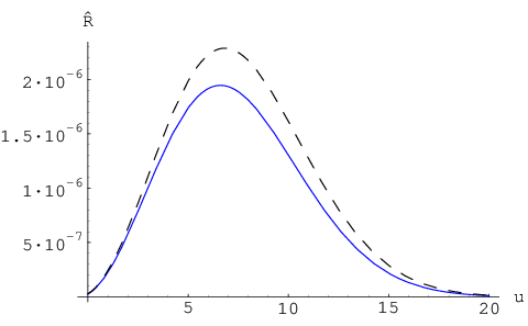 b)
b) 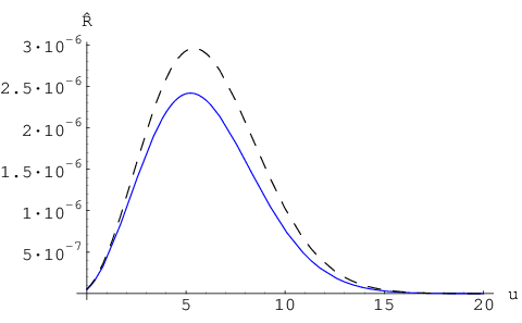
c) 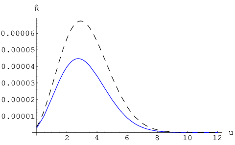
We also examine the accuracy of eq. (47) by plotting in Figure 5 its predicted value for against the actual value obtained numerically from (43).

References
- [1]
J. M. Maldacena,
“The large N limit of superconformal field theories and supergravity,”
Adv. Theor. Math. Phys. 2, 231 (1998)
[Int. J. Theor. Phys. 38, 1113 (1999)]
[arXiv:hep-th/9711200];
S. S. Gubser, I. R. Klebanov and A. M. Polyakov, “Gauge theory correlators from non-critical string theory,” Phys. Lett. B 428, 105 (1998) [arXiv:hep-th/9802109];
E. Witten, “Anti-de Sitter space and holography,” Adv. Theor. Math. Phys. 2, 253 (1998) [arXiv:hep-th/9802150]. - [2] J. Polchinski and M. J. Strassler, “Hard scattering and gauge/string duality,” Phys. Rev. Lett. 88, 031601 (2002) [arXiv:hep-th/0109174].
- [3] J. Polchinski and M. J. Strassler, “Deep inelastic scattering and gauge/string duality,” JHEP 0305, 012 (2003) [arXiv:hep-th/0209211].
- [4] J. B. Kogut and L. Susskind, “Scale invariant parton model,” Phys. Rev. D 9, 697 (1974).
- [5] R. C. Brower, J. Polchinski, M. J. Strassler and C. I. Tan, “The Pomeron and Gauge/String Duality,” JHEP 0712, 005 (2007) [arXiv:hep-th/0603115].
- [6]
L. N. Lipatov,
“Reggeization Of The Vector Meson And The Vacuum Singularity In Nonabelian
Gauge Theories,”
Sov. J. Nucl. Phys. 23, 338 (1976)
[Yad. Fiz. 23, 642 (1976)];
E. A. Kuraev, L. N. Lipatov and V. S. Fadin, “The Pomeranchuk Singularity In Nonabelian Gauge Theories,” Sov. Phys. JETP 45, 199 (1977) [Zh. Eksp. Teor. Fiz. 72, 377 (1977)];
I. I. Balitsky, “Effective Electric Charge And Asymptotic Freedom. (In Russian),” Yad. Fiz. 27, 1091 (1978). - [7] A. A. Affolder et al. [CDF Collaboration], “Observation of diffractive production at the Fermilab Tevatron,” Phys. Rev. Lett. 87, 241802 (2001) [arXiv:hep-ex/0107071].
- [8] J. R. Forshaw, “Diffractive Higgs production: Theory,” arXiv:hep-ph/0508274.
- [9] J. Erlich, E. Katz, D. T. Son and M. A. Stephanov, “QCD and a holographic model of hadrons,” Phys. Rev. Lett. 95, 261602 (2005) [arXiv:hep-ph/0501128].
- [10] L. Da Rold and A. Pomarol, “Chiral symmetry breaking from five dimensional spaces,” Nucl. Phys. B 721, 79 (2005) [arXiv:hep-ph/0501218].
- [11] H. Kawai, D. C. Lewellen and S. H. H. Tye, “A Relation Between Tree Amplitudes Of Closed And Open Strings,” Nucl. Phys. B 269, 1 (1986).
- [12] L. N. Lipatov, “Massless Particle Production in High-Energy Scattering of Strings,” Sov. Phys. JETP 67, 1975 (1988) [Zh. Eksp. Teor. Fiz. 94, 37 (1988)].
- [13] R. C. Brower, C. E. DeTar and J. H. Weis, “Regge Theory For Multiparticle Amplitudes,” Phys. Rept. 14, 257 (1974).
- [14] S. Hong, S. Yoon and M. J. Strassler, “On the couplings of the rho meson in AdS/QCD,” arXiv:hep-ph/0501197.
- [15] S. Hong, S. Yoon and M. J. Strassler, “On the couplings of vector mesons in AdS/QCD,” JHEP 0604, 003 (2006) arXiv:hep-th/0409118.
- [16] S. M. Cohen, “Path integral for the quantum harmonic oscillator using elementary methods,” Am. J. Phys. 66, 537 (1998).
- [17] A. Karch and E. Katz, “Adding flavor to AdS/CFT,” JHEP 0206, 043 (2002) [arXiv:hep-th/0205236].
- [18]
J. Polchinski,
“String theory. Vol. 1: An introduction to the bosonic string,”
Cambridge, UK: Univ. Pr. (1998) 402 p;
J. Polchinski, “String theory. Vol. 2: Superstring theory and beyond,” Cambridge, UK: Univ. Pr. (1998) 531 p. - [19] M. B. Green, J. H. Schwarz and E. Witten, “Superstring Theory. Vol. 1: Introduction,” Cambridge, UK: Univ. Pr. (1987) 469 p.