Gravitating (field theoretical) cosmic (p,q)-superstrings

In the following we shall analyse the system of coupled differential equations associated with the gravitationally coupled system described above. This system will contain the Euler-Lagrange equations for the matter fields and the Einstein equations for the metric fields. In order to do that, let us write down the matter and gravitational fields as shown below. The most general, cylindrically symmetric line element invariant under boosts along the $z-$direction is:

The non-vanishing components of the Ricci tensor $R_{\mu}^{\nu}$ then read [14]:

where the prime denotes the derivative with respect to $\rho$.

For the matter and gauge fields, we have [22]:

$n$ and $m$ are integers indexing the vorticity of the two Higgs fields around the $z-$axis.

We define the following dimensionless variable and function:

Then, the total Lagrangian only depends on the following dimensionless coupling constants

Varying the action with respect to the matter fields and metric functions, we obtain a system of six non-linear differential equations. The Euler-Lagrange equations for the matter field functions read:

where the prime now and in the following denotes the derivative with respect to $x$.

We use the Einstein equations in the following form:

where $T$ is the trace of the energy momentum tensor $T=T^{\lambda}_{\lambda}$ and the non-vanishing components of the energy-momentum tensor are (we use the notation of [14]) with $i=1,2$:

where

and

corresponding to the choice of potential $V_{1}$ and $V_{2}$, respectively.

We then obtain

and:

The requirement of regularity at the origin leads to the following boundary conditions:

for the matter fields and

for the metric fields.

In the special case where $n\neq 0$ and $m=0$ the boundary conditions (24) change according to:

while for a $n=0$, $m\neq 0$ string, they read

By letting the derivatives of the non-winding scalar field be zero at the origin instead of imposing the boundary conditions for the fields themselves, the non-winding scalar field can take non-zero values at the origin and, as it is indeed the case, a “condensate” of the non-winding scalar field will form in the core of the winding string.

The finiteness of the energy per unit length requires:

We define as inertial mass per unit length of the solution

where $g_{3}$ is the determinant of the $2+1$-dimensional space-time given by $(t,x,\varphi)$. This then reads:

As mentioned earlier, for Saffin’s model $V_{1}$, $\beta_{3}=0$ corresponds to two non-interacting strings. In the BPS limit (the limit we are dealing with) the inertial mass (in units of $2\pi$) of the $(1,1)$ string is just $E_{in}(\gamma)=2$. This is because the mass is equal to the sum of the masses of the $(1,0)$-string and of the $(0,1)$-string, which is $E_{in}^{(1,0)}(\gamma)=E_{in}^{(0,1)}(\gamma)=1$. Correspondingly, the deficit angle (in units of $2\pi$) is just $\delta/(2\pi)=2\gamma$.

We can then define the binding energy of an $(n,m)$ string as

The solutions for $\gamma=0$, i.e. in flat space-time have been discussed in [5] and [6]. When $\gamma$ is increased from zero, the (p,q)-strings get deformed by gravity. If $\gamma$ is not too large, globally regular solutions exist. These solutions fall into two categories [14, 15]: the string solutions and the Melvin solutions, where the latter have no flat-space counterpart. The string solutions are those of astrophysical interest since they describe solutions with a deficit angle and because the Melvin solutions are heavier than their string counterparts. The metric functions then have the following behaviour at infinity:

where the $c_{i}$, $i=1,2,3$ are constants that depend on the choice of $\gamma$, $\beta_{i}$, $i=1,2,3$, $q$ and $g$. The solution has a deficit angle which is given by

If the deficit angle $\delta>2\pi$, $c_{2}<0$ and the solution would have a singularity at a finite, parameter-dependent value of $x=x_{0}$ with $L(x=x_{0})=0$, while $N(x_{0})$ stays finite. These solutions are the so-called supermassive string solutions [13] (or inverted string solutions).

The Melvin solutions exist for the same parameter values as the string solutions, but have a different asymptotic behaviour:

where again $a_{1}$ and $a_{2}$ are parameter dependent constants. This latter solution is thus not a cosmic string solution in the standard sense since it corresponds to a solution for which the circumference of circles will decay in the asymptotic region.

The profiles of typical string and Melvin solutions are shown in Fig. 1.

We have solved the above system of equations for $\beta_{i}=2$, $i=1,2$, $g=1$ ( which for $\gamma=0$ corresponds to the BPS limit) and $q=1$. First, we have fixed $\gamma=0.5$ and investigated the dependence of the deficit angle on the binding parameter $\beta_{3}$ and on the choice of $n$ and $m$. Note that in order for $h(x)=1$, $f(x)=1$ to be the global minimum of the theory for our choice of the remaining parameters given above, we have to require $0<\beta_{3}<1$.

Our numerical results are given in Fig. 2. The deficit angle is decreasing for increasing $\beta_{3}$ and tends to zero in the limit $\beta_{3}\rightarrow 1$. This is expected, since the increase of $\beta_{3}$ leads to a stronger binding between the strings, the total energy decreases and thus results in a smaller deficit angle. Moreover, the deficit angle for a fixed value of $\beta_{3}$ is smaller for an $(n,n)$ string than for an $(n+1,n-1)$ string, which itself is smaller than that for an $(n+2,n-2)$ string etc. This is clearly seen for the deficit angle of the $(2,0)$ string in comparison to that of the $(1,1)$ string and accordingly for strings with $n+m=3$ and $n+m=4$, respectively.

It is also obvious from Fig. 2 that globally regular string solutions exist only for a specific parameter range. For $\beta_{3}=0$, the deficit angle is given by $\delta/(2\pi)=(n+m)\gamma$. Since globally regular string solutions exist only for $\delta\leq 2\pi$, we need $(n+m)\gamma\leq 1$ or for $\gamma=0.5$, $n+m\leq 2$. Thus, for our specific choice of $\gamma$ and for $\beta_{3}=0$ we would not expect regular string solutions to exist for $n+m\geq 3$. This is clearly seen in the figure, where string solutions with deficit angle less than $2\pi$ exist for all values of $\beta_{3}$ only for the $(1,0)$, $(1,1)$ and $(2,0)$ cases. However, regular string solutions exist also for $n+m\geq 3$ if $\beta_{3}$ is large enough. For $n+m\geq 3$ and a fixed value of $\gamma$, regular string solutions exist for $\beta_{3}>\beta_{3}^{(cr)}(\gamma,n,m)$. We find e.g. $\beta_{3}^{(cr)}(0.5,2,1)\approx 0.76$, $\beta_{3}^{(cr)}(0.5,3,0)\approx 0.86$, $\beta_{3}^{(cr)}(0.5,2,2)\approx 0.89$ and $\beta_{3}^{(cr)}(0.5,4,0)\approx 0.94$. The value $\beta_{3}^{(cr)}$ increases for $n+m$ increasing, since a higher total winding requires a higher binding energy in order to render the string not too heavy. Moreover, for $(n,m)=(n+k,n-k)$ strings, where $0\leq k\leq n$, the value of $\beta_{3}^{(cr)}$ increases for increasing $k$.

We have also studied the dependence of the deficit angle on the gravitational coupling for a fixed value of $\beta_{3}=0.95$. The results are given in Fig. 3.

As expected the deficit angle increases for increasing $\gamma$ and tends to $2\pi$ for $\gamma\rightarrow\gamma^{(cr)}(\beta_{3},n,m)$. Thus, globally regular strings exist only for $\gamma\leq\gamma^{(cr)}(\beta_{3},n,m)$. This critical value of the gravitational coupling decreases for $n+m$ increasing and for a fixed value of $n+m$ and $(n,m)=(n+k,n-k)$, $0\leq k\leq n$, decreases for $k$ increasing.

Clearly, the specific choice of $\beta_{3}$, $\gamma$ and $(n,m)$ determines whether globally regular solutions with deficit angle smaller than $2\pi$ exist. Increasing $\beta_{3}$ leads to a stronger binding between the strings, i.e. the energy of the $(n,m)$-string is lowered and hence globally regular solutions exist for higher values of $\gamma$. This is demonstrated in Fig. 4 for $(1,0)$, $(1,1)$ and $(2,1)$ strings. Here, we plot the value of the gravitational coupling up to which the regular solutions exist, $\gamma^{(cr)}$, as function of $\beta_{3}$. Note that regular solutions exist only in the parameter domain below the respective curves. It is clear that the solutions exist for higher values of $\gamma$ when $\beta_{3}$ is increased. This is related to the increase in binding energy, e.g. for the $(2,1)$ solution with $\gamma=0.5$, we find that $E_{bin}^{(2,1)}\approx-0.551$ for $\beta_{3}=0.8$, while $E_{bin}^{(2,1)}\approx-0.652$ for $\beta_{3}=0.95$. In addition to the binding due to the potential, there is an additional binding due to gravity. The larger $\gamma$, the stronger is the binding: e.g. for $\beta_{3}=0.9$, we find $E_{bin}^{(2,1)}\approx-0.621$ for $\gamma=0.5$, while $E_{bin}^{(2,1)}\approx-0.581$ for $\gamma=0$, in agreement with what it has been reported [5].

First, we have studied the solutions for $\tilde{\beta}_{1}=\tilde{\beta}_{2}=1$, $q=g=1$ and $\gamma=0.5$ to understand what qualitative differences appear in comparison to the potential $V_{1}$. While in the case of the $V_{1}$ potential (and in the BPS limit) a $(1,0)$-string is exactly equivalent to a $(0,1)$ string, this is different here. As in the $V_{1}$ case, when one string is winding and the other is not, the non-winding string can form a condensate at the core of the other string. However, in this case, a condensate of the $\xi$ field in the core of a $\phi$ string does not lower the energy; whereas a condensate of the $\phi$ inside the $\xi$ core does. More specifically, for $n=1$, $m=0$, the scalar field function $f(x)$ is not forced to zero at the origin and could develop a condensate. However, $f(x)\equiv q$ everywhere and correspondingly $R(x)=0$ gives the minimum for the potential for the boundary conditions we have. On the other hand, for $n=0$ and $m=1$, the scalar field function $h(x)$ is also not forced to zero at the origin, but does develop a condensate. At the origin, a value of $h(x)<1$ is the value that minimizes the energy best. Thus, a $(1,0)$-string is different from a $(0,1)$ string. This can also be seen when looking at the numerical values of the energies and deficit angles. For $(1,0)$, we find $E_{in}\approx 0.859$ and $\delta/(2\pi)\approx 0.425$, while for $(0,1)$, we have $E_{in}\approx 0.848$ and $\delta/(2\pi)\approx 0.418$ (see also Fig. 7).

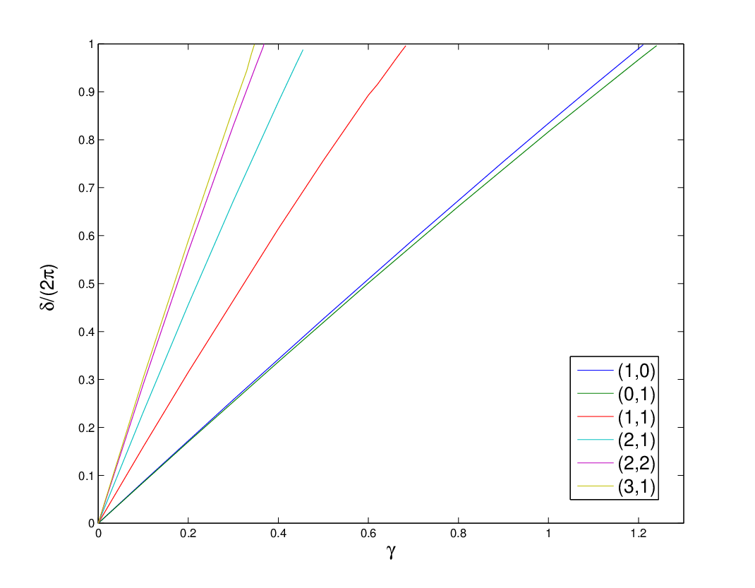
In Fig. 5 we show the dependence of the deficit angle on the gravitational coupling $\gamma$. This is qualitatively very similar to the case with the $V_{1}$ potential. Again, we observe that globally regular string like solutions exist only up to a maximal value of the gravitational coupling $\gamma=\gamma^{(cr)}(n,m)$. If one would increase $\gamma$ further, the solutions would have a deficit angle $>2\pi$ and would thus be singular. $\gamma^{(cr)}(n,m)$ decreases for $n+m$ increasing and for a fixed value of $n+m$ and $(n,m)=(n+k,n-k)$, $0\leq k\leq n$, decreases for $k$ increasing.

As for the $V_{1}$ case, the specific choice of $\beta_{3}$, $\gamma$ and $(n,m)$ determines, whether globally regular solutions exist. The fact that the strings interact and form bound states, lowers their energy. Therefore, for values of $\gamma$ and $(n,m)$ where one would not expect regular global solution in the non-interacting case, regular solutions exists when strings interact.

We have also studied the corresponding Melvin solutions for both potentials. Like their string counterparts, they exist only in a limited domain of the parameter plane.

In the $V_{1}$ case, for a fixed value of $\gamma$, $\beta_{3}^{(cr)}$ is equal for the string and Melvin solutions. This has already been observed in the case of a single gravitating string [14, 15]. At this $\beta_{3}^{(cr)}$, the inertial energies $E_{in}$ of the two types of solutions become equal. This is shown in Fig. 6 for $(n,m)=(3,0)$ and $(n,m)=(2,1)$, respectively. At the critical value of $\beta_{3}^{(cr)}$ the curves of the inertial energies of the two types of solutions merge. Note also that for all cases studied in this paper, the inertial energy of the Melvin solutions is larger than that of the corresponding string solutions.

For $\beta_{3}<\beta_{3}^{(cr)}$, the string solutions become inverted/supermassive string solutions with a zero of the function $L(x)$ at some parameter dependent value of $x=x_{0}$, while $N(x=x_{0})$ stays finite. The Melvin solutions - on the other hand - become so-called Kasner solutions with $N(x=\tilde{x}_{0})=0$ and $L(x\rightarrow\tilde{x}_{0})\rightarrow\infty$ at some finite and parameter-dependent value of $x=\tilde{x}_{0}$. The inverted string and Kasner solutions thus exist only on a finite range of the coordinate $x$ and are thus sometimes also called “closed” solutions. These solutions have singularities in their metric, and it is out of the scope of this paper to investigate their implications.

We have also studied the Melvin solutions in the case of $V_{2}$. Again, the qualitative results are very similar to the case with $V_{1}$. In Fig. 7, we show the dependence of the inertial energy $E_{in}$ on the gravitational coupling $\gamma$ for $\tilde{\beta}_{1}=\tilde{\beta}_{2}=1$, $q=g=1$ and three different choices of $(n,m)$. The inertial energy of the string solutions is always lower than that of the Melvin solutions and the two branches of solutions meet at $\gamma^{(cr)}$, the maximal value of the gravitational coupling, beyond which no globally regular solutions exist. As before, the maximal value of the gravitational coupling decreases with $n+m$ increasing. We include both $(1,0)$ and $(0,1)$ solutions, since, as stated above, the do differ for the $V_{2}$ case.

It has been observed previously [15] that the inertial energy of the Melvin solutions doesn’t depend strongly on the winding number. The reason for this is that the main contribution to the energy of the Melvin solution comes from the gravitational field and is thus “insensitive” to the actual core structure of the solution. This explains why the energy of the Melvin solution practically doesn’t depend on $\beta_{3}$ (see Fig. 6), while it has a strong dependence on the gravitational coupling (see Fig. 7). One could see these effects by studying the gravitationally active mass, the so-called Tolman mass $M_{tol}$ [23], which for our definition of the metric is given by [14]: $M_{tol}\propto{\rm lim}_{x\rightarrow\infty}(LNN^{\prime})$. Clearly, for the standard string solutions, this mass is zero, while for the Melvin solutions it is non-vanishing. The Tolmann mass of the Melvin solutions would then depend on the windings of the strings (see also the discussions in [15]).