Queueing systems with pre-scheduled random arrivals

G. Guadagni S. Ndreca B.Scoppola

August 24, 2026

Abstract

We consider a point process $i+\xi_{i}$ , where $i\in{\mathbb{Z}}$ and the $\xi_{i}$ ’s are i.i.d. random variables with variance $\sigma^{2}$ . This process, with a suitable rescaling of the distribution of $\xi_{i}$ ’s, converges to the Poisson process in total variation for large $\sigma$ . We then study a simple queueing system with our process as arrival process, and we provide a complete analytical description of the system. Although the arrival process is very similar to the Poisson process, due to negative autocorrelation the resulting queue is very different from the Poisson case. We found interesting connections of this model with the statistical mechanics of Fermi particles. This model is motivated by air traffic systems.

†Department of Mathematics, University of Virginia

email: guadagni@virginia.edu

‡Dipartimento di Matematica, Università di Roma “Tor Vergata”

e-mail: ndreca@mat.uniroma2.it, scoppola@mat.uniroma2.it

Keywords: Queueing system, air-traffic congestion, non Poissonian arrivals.

1 Introduction

The main aim of this paper is to define a stochastic point process to model the arrivals to a queueing system, and to compare its features to the Poisson process.

It is well known that the memoryless property of the Poisson process simplifies many technical steps in the analysis of queueing systems, but there are arrival processes where such an assumption is not completely satisfied. In particular, we have in mind air traffic models. In recent times the dramatic increase of air traffic stimulated a large number of studies concerning the optimization of congestion management. From the point of view of classical queueing theory the system is difficult to study, mainly because it is hard even to define the basic quantities of the theory. For instance it is clear that there is some congestion for landing aircrafts, since they have to follow some holding paths, but it is not easy to quantify the actual time spent in queue or even its instant length. On the other hand, even assuming that the parameters of the system are known, it is not clear what kind of point processes are suitable to describe arrivals and service times. A common hypothesis in literature is to assume that arrivals are very well modeled by a Poisson process. This assumption, to our knowledge, goes back to the 70’s when Dunlay and Horonjeff gave in [7] a number of theoretical and statistical arguments to justify the Poissonian hypothesis, and , since then, several other statistical studies have supported the same results. Even recently, see [6], a very careful study of the interarrival times of aircrafts to major US airports shows a small difference between the Poisson and the observed distribution, i.e. the actual arrivals are slightly less random than Poissonian ones, but the difference is quite small in all observed airports. On this ground, in various papers, see for instance [8], [9] and [10] and reference therein, Poisson arrivals have been assumed in the analysis of judicious management of service times. It should be stressed that in all these papers the statistical validation of the Poissonian hypothesis has been based on computations on time scales smaller than the intrinsic randomness of the system.

Stochastic models of aircraft arrivals based on statistical analysis and on simulations have a long history. As a first attempt, Barnett et al. [1] studied the arrivals to Boston Logan Airport. A version of the alternative model of arrivals we propose in this paper was introduced and studied numerically in [4]. The model is refined in [3], where seasonal and daily effects are taken into account to describe random delays of departure times and, with these corrections, the model is quite accurate in its predictions. The key feature of the model is a soft a-priori scheduling of arrivals: indeed, both in US and in Europe, aircrafts are supposed to take off and to land by a schedule dictated by the capacity constraint of the runways, and by the assumption that each aircraft would land in a very narrow time slot. However, on the day of operations, an aircraft will be declared ”on time” if it lands in a time interval larger than ten times the original slot. In this sense the scheduling should be considered ”soft”. The fact that arrivals are prescheduled clearly makes the Poissonian hypothesis questionable, but this is usually neglected, on the basis of the statistical studies mentioned above. However the predictions of the queueing theory give in general very rough estimates of the actual queue length. Moreover if we forecast a reduction of the intrinsic variability of arrival times, which could be achieved by various technical improvements (e.g. a rescheduling closer to the actual arrival times, or an en-route control of the paths of the aircrafts), we can not use Poissonian arrivals to describe the system, because they depend only on a single parameter $\rho$ .

The process we study below is an arrivals model with two features. First, it shows a pattern of arrivals very close to a Poisson process when we look at time scales smaller than the standard deviation of aircraft delays, second, it provides the distribution of arrivals on time scales larger or comparable to the standard deviation of aircraft delays.

Thus, the aim of this paper is an attempt to study more rigorously the features of arrival process presented in [4], which we suitably generalize, and to understand its analytical properties.

Moreover, we show, both analytically and numerically, that the congestion related to this process is very different from the congestion of a Poisson process, on any time scale. This is due to the negative autocorrelation of the process, as we prove explicitly. It is worth to outline that the queueing models with Poisson arrivals have in general probabilities to have $n$ customers in the queue that decay much slower than the probabilities observed in the air traffic. Our model gives a tail of the distribution much thinner, and more similar to the observed data.

The analytical description of the system clarifies many interesting features of this kind of traffic: for heavy traffic the system has a long memory of the initial conditions; its description is obtained by the superposition of two processes, living on different time scales. This give the possibility to investigate also systems with slowly variable traffic intensities.

The paper is organized as follows: in section 2 we describe our arrival process, and we list some results on the comparison to the Poisson process. In section 3 we present a simplified computation, obtained neglecting the autocorrelation of the process.The congestion levels according to this approximated process, assuming deterministic service (landing) times and a single server (runway), are quite different from the congestion according to Poisson arrivals. However we show numerically that such approximation is bad for very congested systems, where the actual level of congestion is not well described if the autocorrelation of the process is neglected. In section 4 we describe completely our queueing system at the price to enlarge suitably the state space of the Markov chain describing it. It turns out that for our process we have a finite value of the expected queue length even in the critical case ${\varrho}=1$ , while the Poisson queue diverges. Starting from the results on the critical case, we propose an approximation scheme that works very well for highly congested ( ${\varrho}$ near to 1) systems. In this description a nice connection with the statistical mechanics of Fermi gas emerges quite naturally. Section 5 is devoted to conclusions and open problems.

2 Description of the model: the arrival process

In this section we want to introduce an arrival process, which we will call pre-scheduled random arrivals (PSRA) process, and to study its main features. The PSRA process is defined as follows. Let $\frac{1}{\lambda}$ be the expected interarrival time between two clients, we define $t_{i}\in\mathbb{R}$ the actual arrival time of the $i$ -th client by

t_{i}={i\over{\lambda}}+\xi_{i}\qquad i\in\mathbb{Z}

(2.1)

where $\xi_{i}$ ’s are i.i.d. random variables.

If the $\xi_{i}$ ’s are uniform, the model is the actual arrival times process introduced in [4] without cancellations and pop-ups. We will show later that cancellations and pop-ups can be easily integrated into the process. From now on, we will assume that $\xi_{i}$ ’s have continuous probability density $f^{({\sigma})}_{\xi}(t)$ with variance $\sigma^{2}$ , and we will set without loss of generality $E(\xi_{i})=0$ , since $E(\xi_{i})\neq 0$ affects only the initial configuration of the system. The main aim of this section is to compare the features of the PSRA process to the Poisson process when $\sigma$ is large. It is well known, e.g. [2, p.447], that the Poisson arrival process is defined by the fact that probabilities $P_{j,j+1}({\Delta}t)=P(n(t+{\Delta}t)=j+1|n(t)=j)$ of a ”jump” from the state $j$ to the state $j+1$ in the time interval $(t,t+{\Delta}t]$ have the form

P_{j,j+1}({\Delta}t)=P^{+}({\Delta}t)={\lambda}{\Delta}t+o({\Delta}t)

(2.2)

where ${\lambda}$ is a constant independent of $t$ and $j$ ; ${\lambda}$ has the meaning of velocity of arrivals, i.e. denoting with $t_{a}$ the interarrival time, $E(t_{a})=\frac{1}{\lambda}$ . For PSRA the probability $P(i,t,{\Delta}t)$ that the $i$ -th client arrives in the time interval $(t,t+{\Delta}t]$ is given by

	$\displaystyle P(i,t,{\Delta}t)$	$\displaystyle=P\left(t<{i\over{\lambda}}+\xi_{i}<t+{\Delta}t\right)=$		(2.3)
		$\displaystyle=P\left(t-{i\over{\lambda}}<\xi_{i}<t+{\Delta}t-{i\over{\lambda}}\right)=\int_{t-{i\over{\lambda}}}^{t+{\Delta}t-{i\over{\lambda}}}f^{({\sigma})}_{\xi}(x)dx$		(2.4)

and, for small ${\Delta}t$ , it may be written as

P(i,t,{\Delta}t)=f^{({\sigma})}_{\xi}\left(t-{i\over{\lambda}}\right){\Delta}t+o({\Delta}t)

(2.5)

By (2.5), the probability $P^{+}(t,{\Delta}t)$ of a single PSRA arrival in the interval $(t,t+{\Delta}t]$ is

P^{+}(t,{\Delta}t)=\sum_{i\in\mathbb{Z}}P(i,t,{\Delta}t)\prod_{j\neq i}(1-P(j,t,{\Delta}t))=

=\sum_{i\in\mathbb{Z}}\left[f^{({\sigma})}_{\xi}\left(t-{i\over{\lambda}}\right){\Delta}t+o({\Delta}t)\right]\exp\left(\sum_{j\neq i}\log\left[1-f^{({\sigma})}_{\xi}\left(t-{j\over{\lambda}}\right){\Delta}t+o({\Delta}t)\right]\right)=

=\sum_{i\in\mathbb{Z}}\left[f^{({\sigma})}_{\xi}\left(t-{i\over{\lambda}}\right){\Delta}t+o({\Delta}t)\right]\exp\left(-\sum_{j\neq i}\left[f^{({\sigma})}_{\xi}\left(t-{j\over{\lambda}}\right){\Delta}t+o({\Delta}t)\right]\right)

(2.6)

Hence up to the first order in ${\Delta}t$ the rate of arrival ${\lambda}(t)$ of the pre-scheduled random arrivals is defined by

{\lambda}(t)=\sum_{i\in\mathbb{Z}}f^{({\sigma})}_{\xi}\left(t-{i\over{\lambda}}\right)

(2.7)

This rate ${\lambda}(t)$ is periodic in $t$ with period $\frac{1}{\lambda}$ . However we are interested in the dependence of ${\lambda}(t)$ on ${\sigma}$ , in particular when ${\sigma}$ is large with respect to $\frac{1}{\lambda}$ . To prove limit properties for our process, we have to specify the way we want to send $\sigma$ to infinity. We will require the following scaling property for the density $f^{(\sigma)}_{\xi}(t)$ .

Assumption 2.1.

The probability density of $\xi$ has the form

f^{({\sigma})}_{\xi}(t,{\sigma}^{2})=\frac{1}{\sigma}f_{\xi}(t/{\sigma})

(2.8)

i.e. it is the rescaling of a well defined continuous density $f_{\xi}(t)$ with finite variance. We will also write $\max_{t\in{\mathbb{R}}}f_{\xi}(t)=M$ .

This assumption is introduced in order to exclude pathological ways to send $\sigma$ to infinity, as, for instance, to consider a bimodal distribution with fixed maxima, see figure 1.

Refer to caption — Figure 1: A bimodal distribution with fixed shapes shifting to infinity for ${\sigma}\rightarrow\infty$ .

By our assumption, it follows that, in the limit ${\sigma}$ very large the expression

R(\sigma,1/{\lambda}):=\sum_{i\in\mathbb{Z}}{1\over{\lambda}}f^{({\sigma})}_{\xi}\left(t-{i\over{\lambda}}\right)

(2.9)

is the Riemann integral of the function $f^{({\sigma})}_{\xi}(t)$ .

For example, let $\xi$ be Gaussian $N(0,\sigma^{2})$ ,

R(\sigma,1/{\lambda})=\sum_{i\in\mathbb{Z}}{1\over\lambda}\frac{1}{\sqrt{2\pi\sigma^{2}}}e^{-\frac{(\lambda t-i)^{2}}{2\sigma^{2}\lambda^{2}}}=\sum_{i\in\mathbb{Z}}\frac{1}{\sqrt{2\pi}}e^{-\frac{1}{2}\left(\frac{t\lambda-i}{\lambda\sigma}\right)^{2}}\frac{1}{\lambda\sigma}=\sum_{i\in\mathbb{Z}}\frac{1}{\sqrt{2\pi}}e^{-\frac{x_{i}^{2}}{2}}\Delta x\longrightarrow 1

where $x_{i}=\frac{\lambda t-i}{\lambda\sigma}$ and $\Delta x=\frac{1}{\lambda\sigma}$ and the limit is for $\sigma\rightarrow\infty$ .

For any random variable rescaled in the above sense it is clear that the result

\lim_{{\sigma}\to\infty}R(\sigma,1/{\lambda})=1

(2.10)

holds, and therefore, in the same limit,

\lim_{{\sigma}\to\infty}{\lambda}(t)=\lim_{{\sigma}\to\infty}\lambda R(\sigma,1/{\lambda})={\lambda}

(2.11)

It is interesting, for Gaussian $\xi$ , to check numerically how fast the limit is reached. Table 1 shows it. For simplicity, we set ${\lambda}=1$ .

${\sigma}$	${\lambda}(0)$	${\lambda}(0.1)$	${\lambda}(0.2)$	${\lambda}(0.3)$	${\lambda}(0.4)$	${\lambda}(0.5)$
.2	1.994726	1.760407	1.210523	0.651951	0.292114	0.175283
.3	1.340089	1.274318	1.103259	0.894087	0.726696	0.663191
.4	1.085005	1.068767	1.026261	0.973729	0.931237	0.915008
.5	1.014384	1.011637	1.004445	0.995555	0.988363	0.985616
.6	1.00164	1.001327	1.000507	0.999493	0.998673	0.99836
.7	1.000126	1.000102	1.000039	0.999961	0.999898	0.999874
.8	1.000007	1.000005	1.000002	0.999998	0.999995	0.999993
.9	1.	1.	1.	1.	1.	1.
1.	1.	1.	1.	1.	1.	1.

${\sigma}$	${\lambda}(0.6)$	${\lambda}(0.7)$	${\lambda}(0.8)$	${\lambda}(0.9)$	${\lambda}(1)$
.2	0.292114	0.651951	1.210523	1.760407	1.994726
.3	0.726696	0.894087	1.103259	1.274318	1.340089
.4	0.931237	0.973729	1.026261	1.068767	1.085005
.5	0.988363	0.995555	1.004445	1.011637	1.014384
.6	0.998673	0.999493	1.000507	1.001327	1.00164
.7	0.999898	0.999961	1.000039	1.000102	1.000126
.8	0.999995	0.999998	1.000002	1.000005	1.000007
.9	1.	1.	1.	1.	1.
1.	1.	1.	1.	1.	1.

Table 1:

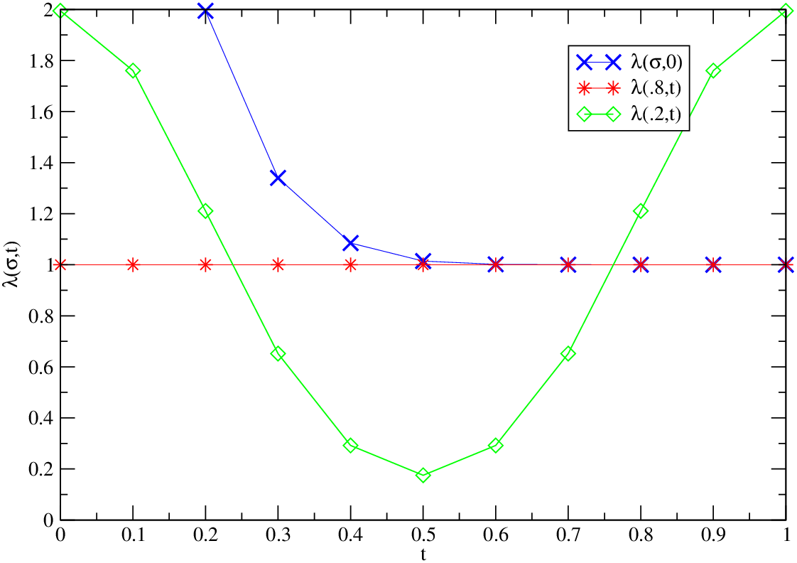
The graph in figure 2 shows that, in terms of rate of arrivals, the pre-scheduled random arrivals approach the Poisson process when ${\sigma}$ is suitably large. In particular for Gaussian variables with standard deviation ${\sigma}$ of order $1/{\lambda}$ or more we have that ${\lambda}(t)$ is constant up to 6 digits. Note that for applications mentioned in the introduction, we do expect the standard deviation to be much larger than $1/{\lambda}$ . Note also that the explicit structure of the density of $\xi$ does not play any particular role, and similar results may be obtained with different distributions. However it is clear that a small dependence on $t$ is always present in the expression of ${\lambda}(t)$ , and hence it is difficult to obtain a quantitative comparison between the pre-scheduled random arrivals and the Poisson process on this basis. Hence we look at the distribution of the random variable $n(t,t+T)$ , number of arrivals in the finite interval $(t,t+T]$ . Let us call $p_{i}(t,t+T)$ the probability that the $i$ -th client arrives in the interval $(t,t+T]$ . Clearly

p_{i}(t,t+T)=\int_{t}^{t+T}f^{(\sigma)}_{\xi}\left(x-{i\over{\lambda}}\right)dx

(2.12)

Given the probabilities $p_{i}(t,t+T)$ we can write the generating function of the random variable $n(t,t+T)$ , and, defining $q_{n}^{({\sigma})}=P(n(t,t+T)=n)$ we get

q_{n}^{({\sigma})}=\sum_{I=\{i_{1},...,i_{n}\}}\prod_{i\in I}p_{i}(t,t+T)\prod_{j\notin I}(1-p_{j}(t,t+T))

(2.13)

where the sum runs over all the possible distinct subsets $I$ of indices of cardinality $n$ . By mean of this expression one obtains the generating function

q^{({\sigma})}(z)=\sum_{n\geq 0}q_{n}^{({\sigma})}z^{n}=\prod_{i\in\mathbb{Z}}(1+(z-1)p_{i}(t,t+T))

(2.14)

To take into account also the possibility of random independent deletion as in [4], let us outline here that a similar generating function can be introduced also when each arrival has an independent probability $1-\gamma$ to be deleted, and the complementary probability $\gamma$ to be an actual arrival. In other words, we construct the PSRA process for $i\in\mathbb{Z}$ and then for each $i$ we cancel the corresponding $i$ -th arrival with independent probability $1-\gamma$ . It is obvious that in this case the generating function is

q^{({\sigma})}_{\gamma}(z)=\sum_{n\geq 0}q_{\gamma,n}^{({\sigma})}z^{n}=\prod_{i\in\mathbb{Z}}(1+(z-1)\gamma p_{i}(t,t+T))

(2.15)

The expressions (2.14), (2.15) are exact, they give us all the information on the distribution of $n(t,t+T)$ , and they depend explicitly on $t$ and $T$ . However we want to study $q^{({\sigma})}(z)$ and $q^{({\sigma})}_{\gamma}(z)$ for large ${\sigma}$ , in the sense of the rescaling defined above, showing that they converge to a Poisson distribution with parameter ${\lambda}T$ and $\gamma{\lambda}T$ respectively. The main idea is to exploit the fact that, for large ${\sigma}$ , $p_{i}(t,t+T)$ goes to zero as ${1\over{\sigma}}$ .

We now prove the following results.

Lemma 2.2.

\max_{i}p_{i}(t,t+T)\leq\frac{{const(T)}}{{\sigma}}

(2.16)

Proof.

p_{i}(t,t+T)=\int_{t}^{t+T}f^{({\sigma})}_{\xi}\left(x-{i\over{\lambda}}\right)dx=\int_{t-\frac{i}{{\lambda}}}^{t-\frac{i}{{\lambda}}+T}f^{({\sigma})}_{\xi}(s)ds={1\over{\sigma}}\int_{{t}-\frac{i}{{\lambda}}}^{{t}-\frac{i}{{\lambda}}+{T}}f_{\xi}\left({s\over{\sigma}}\right)ds

(2.17)

by the Intermediate Value Theorem

p_{i}(t,t+T)={1\over{\sigma}}f_{\xi}\left({s_{i}^{*}\over{\sigma}}\right){T}\leq{MT\over{\sigma}}

(2.18)

where

\frac{s_{i}^{*}}{\sigma}\in\left(t-\frac{i}{\lambda},t-\frac{i}{\lambda}+T\right)

∎

Now we will use lemma 2.2 to bound the generating function

	$\displaystyle q^{(\sigma)}(z)=\exp\left[\sum_{i\in\mathbb{Z}}\ln(1+(z-1)p_{i}(t,t+T))\right]=$		(2.19)
	$\displaystyle=\exp\left[(z-1)\sum_{i\in\mathbb{Z}}p_{i}(t,t+T)\left(1+(z-1)p_{i}(t,t+T)\int_{0}^{1}ds\frac{s}{(1+(z-1)(1-s)p_{i}(t,t+T))^{2}}\right)\right]$		(2.20)

Lemma 2.3.

With $p_{i}(t,t+T)$ defined as above, the sum in (2.20) converges to $\lambda T$

\lim_{{\sigma}\to\infty}\sum_{i\in\mathbb{Z}}p_{i}(t,t+T)\left(1+(z-1)p_{i}(t,t+T)\int_{0}^{1}ds\frac{s}{(1+(z-1)(1-s)p_{i}(t,t+T))^{2}}\right)={\lambda}T

(2.21)

Proof.

First we prove that

\lim_{{\sigma}\to\infty}\sum_{i\in\mathbb{Z}}p_{i}(t,t+T)={\lambda}T.

(2.22)

Let us define $T:=\frac{K+{\Delta}T}{{\lambda}}$ , where $K\in\mathbb{Z^{+}}$ and $0\leq{\Delta}T<1$ . Then we can write

\sum_{i\in\mathbb{Z}}p_{i}(t,t+T)=\sum_{i\in\mathbb{Z}}\int_{t-\frac{i}{{\lambda}}}^{t-\frac{i}{{\lambda}}+T}f^{({\sigma})}_{\xi}(s)ds=\sum_{i\in\mathbb{Z}}\int_{t-\frac{i}{{\lambda}}}^{t+\frac{K-i}{{\lambda}}+{{\Delta}T\over{\lambda}}}f^{({\sigma})}_{\xi}(s)ds=

=\sum_{i\in\mathbb{Z}}\int_{t-\frac{i}{{\lambda}}}^{t+\frac{K-i}{{\lambda}}}f^{({\sigma})}_{\xi}(s)ds+\sum_{i\in\mathbb{Z}}\int_{t+\frac{K-i}{{\lambda}}}^{t+\frac{K-i}{{\lambda}}+{{\Delta}T\over{\lambda}}}f^{({\sigma})}_{\xi}(s)ds

(2.23)

The first term on the right hand side of (2.23) is $K$ . Let $i=mK+l$ , where $l\in\mathbb{Z^{+}}$ and $m\in\mathbb{Z}$ ,

\sum_{i\in\mathbb{Z}}\int_{t-\frac{i}{{\lambda}}}^{t+\frac{K-i}{{\lambda}}}f^{({\sigma})}_{\xi}(s)ds=\sum_{l=0}^{K-1}\sum_{m\in\mathbb{Z}}\int_{t-\frac{mK+l}{{\lambda}}}^{t-\frac{(m-1)K+l}{{\lambda}}}f^{({\sigma})}_{\xi}(s)ds=\sum_{l=0}^{K-1}\int_{\mathbb{R}}f^{({\sigma})}_{\xi}(s)ds=K

(2.24)

The second term on the right hand side of (2.23) converges to ${\Delta}T$ for ${\sigma}\rightarrow\infty$ :

\sum_{i\in\mathbb{Z}}\int_{t+\frac{K-i}{{\lambda}}}^{t+\frac{K-i}{{\lambda}}+{{\Delta}T\over{\lambda}}}f^{({\sigma})}_{\xi}(s)ds=\sum_{i\in\mathbb{Z}}\int_{t+\frac{i}{{\lambda}}}^{t+\frac{i}{{\lambda}}+{{\Delta}T\over{\lambda}}}f^{({\sigma})}_{\xi}(s)ds=\sum_{i\in\mathbb{Z}}{1\over{\sigma}}\int_{{t}+\frac{i}{{\lambda}}}^{{t}+\frac{i}{{\lambda}}+{{\Delta}T\over{\lambda}}}f_{\xi}\left({s\over{\sigma}}\right)ds

(2.25)

and, by the Intermediate Value Theorem we get

\sum_{i\in\mathbb{Z}}{1\over{\sigma}}\int_{t+\frac{K-i}{{\lambda}}}^{t+\frac{K-i}{{\lambda}}+{{\Delta}T\over{\lambda}}}f_{\xi}\left({s\over{\sigma}}\right)ds=\sum_{i\in\mathbb{Z}}{1\over{\sigma}}f_{\xi}\left({s_{i}^{*}\over{\sigma}}\right){{\Delta}T\over{\lambda}}={\Delta}T\sum_{i\in\mathbb{Z}}f_{\xi}\left({s_{i}^{*}\over{\sigma}}\right){1\over{\lambda}{\sigma}}\longrightarrow{\Delta}T

(2.26)

as ${\sigma}\to\infty$ , where the sum on the last equality is the Riemann sum of $f_{\xi}(t)$ . This ends the proof of (2.22). In order to complete the lemma we need to show that, uniformly in $i$ ,

\lim_{{\sigma}\to\infty}(z-1)p_{i}(t,t+T)\int_{0}^{1}ds\frac{s}{(1+(z-1)(1-s)p_{i}(t,t+T))^{2}}=0

but this follows from lemma 2.2 and from the fact that

(z-1)\int_{0}^{1}ds\frac{s}{(1+(z-1)(1-s)p_{i}(t,t+T))^{2}}\leq C

for any $p_{i}(t,t+T)<1/2$ and $|z|\leq 1$ .

∎

Lemma 2.4.

Let $q(z)=\exp({{\lambda}T(z-1)})$ be the probability generating function of the Poisson random variable ${\zeta}$ with intensity ${\lambda}T$ , and $q_{\gamma}(z)=\exp({\gamma{\lambda}T(z-1)})$ be the probability generating function of the Poisson random variable ${\zeta}$ with intensity $\gamma{\lambda}T$ , then

\lim_{{\sigma}\to\infty}q^{({\sigma})}(z)=q(z);\quad\lim_{{\sigma}\to\infty}q_{\gamma}^{({\sigma})}(z)=q_{\gamma}(z)

(2.27)

Proof.

Follows immediately from lemma 2.3. ∎

Theorem 2.5.

If $q^{({\sigma})}(z)\longrightarrow q(z)$ , then $\sum_{n=0}^{\infty}|q_{n}^{({\sigma})}-q_{n}|\longrightarrow 0$ as ${\sigma}\to\infty$ . The same result holds for the arrivals with random deletions.

Proof.

The proof follows from the continuity theorem for probability generating function see Feller [2, p.280]. ∎

Hence the PSRA process converges in distribution to the Poisson process in total variation norm, and the same is true for PSRA process with independent random deletions.

In order to show that the process has negative autocorrelation, we will compute the expected value, the variance $Var(n)$ of the number $n$ of arrivals in a time slot $(t,t+T]$ , and the covariance $Cov(n_{1},n_{2})$ , where $n_{1}$ and $n_{2}$ are the numbers of arrivals in $(t,t+T]$ and $(t+T,t+2T]$ , respectively. We present the explicit computations in the case of simple PSRA process, but the same results are true with obvious modifications for PSRA process with independent random deletions.
Let $\chi_{i}(t_{i}\in(t,t+T])$ be the characteristic function of the event “client $i$ arrives in the interval $(t,t+T]$ ”, so that ${\mathbb{E}}(\chi_{i})=p_{i}(t,t+T)$ , then the expected number of arrivals in a time slot $(t,t+T]$ is

{\mathbb{E}}(n)={\mathbb{E}}\left(\sum_{i}\chi_{i}\right)=\sum_{i}{\mathbb{E}}(\chi_{i})=\sum_{i}p_{i}(t,t+T)

and also

	$\displaystyle{\mathbb{E}}(n^{2})$	$\displaystyle={\mathbb{E}}\left(\sum_{i}\chi_{i}\sum_{j}\chi_{j}\right)={\mathbb{E}}\left(\sum_{i}\chi_{i}+\sum_{i\neq j}\chi_{i}\chi_{j}\right)=$
		$\displaystyle=\sum_{i}p_{i}(t,t+T)+\sum_{i\neq j}p_{i}(t,t+T)p_{j}(t+T,t+2T)$
		$\displaystyle=\sum_{i}p_{i}(t,t+T)+\left(\sum_{i}p_{i}(t,t+T)\right)^{2}-\sum_{i}(p_{i}(t,t+T))^{2}$

Then the variance is:

Var(n)={\mathbb{E}}(n^{2})-({\mathbb{E}}(n))^{2}=\sum_{i}p_{i}(t,t+T)-\sum_{i}(p_{i}(t,t+T))^{2}=\sum_{i}p_{i}(t,t+T)(1-p_{i}(t,t+T))

and we see again that $Var(n)\rightarrow\lambda T$ in the limit ${\sigma}\rightarrow\infty$ . Finally, let us define $\chi_{i}^{(1)}:=\chi_{i}(t_{i}\in(t,t+T])$ and $\chi_{i}^{(2)}:=\chi_{i}(t_{i}\in(t+T,t+2T])$

	$\displaystyle{\mathbb{E}}(n_{1}n_{2})$	$\displaystyle={\mathbb{E}}\left(\sum_{i}\chi^{(1)}_{i}\sum_{j}\chi^{(2)}_{j}\right)={\mathbb{E}}(\sum_{i\neq j}\chi_{i}^{(1)}\chi_{j}^{(2)})=\sum_{i\neq j}{\mathbb{E}}(\chi_{i}^{(1)}){\mathbb{E}}(\chi_{j}^{(2)})=$
		$\displaystyle=\sum_{i\neq j}p_{i}(t,t+T)p_{j}(t+T,t+2T)$
		$\displaystyle=\sum_{i,j}p_{i}(t,t+T)p_{j}(t+T,t+2T)-\sum_{i}p_{i}(t,t+T)p_{i}(t+T,t+2T)$

so that

Cov(n_{1},n_{2})={\mathbb{E}}(n_{1}n_{2})-{\mathbb{E}}(n_{1}){\mathbb{E}}(n_{2})=-\sum_{i}p_{i}(t,t+T)p_{i}(t+T,t+2T)

A negative covariance means that $n_{1}$ and $n_{2}$ are inversely correlated, as we should expect in our arrival model: a congested time slot should be followed or preceded by a slot with lower than expected arrivals. Moreover, this is a clear indication that the hypothesis of independence for $n_{1}$ and $n_{2}$ , numbers of arrivals in different time slots, is not correct, unless we are in the limit $\sigma\rightarrow\infty$ .

3 Queueing systems with PSRA process: independence approximation

In this section we want to try to use the classical results of queueing theory for a system in which the arrivals are described in terms of our PSRA, there is a single server and the service time is deterministic. For the air traffic applications the deterministic service (landing) times are obviously an approximation, but neglecting the mix of aircrafts the actual landing times have a low variability.

In order to study our queueing process we set a service time $T$ and we define the instant traffic intensity ${\varrho}({\sigma},t)=E(n(t,t+T))$ . In fig. 3 and table 2 we report numerical results for the convergence of ${\varrho}({\sigma},t)$ to ${\lambda}T$ , granted by lemma 2.3. For simplicity we consider ${\xi}$ Gaussian, and ${\lambda}=1$ . In this case ${\varrho}({\sigma},t)$ converges as soon as ${\sigma}$ gets close to 1.

${\sigma}$	$T$	${\varrho}({\sigma},0)$	${\varrho}({\sigma},0.1)$	${\varrho}({\sigma},0.2)$	${\varrho}({\sigma},0.3))$	${\varrho}({\sigma},0.4))$
.2	.9	0.808534	0.808534	0.850089	0.907951	0.954826
.3	.9	0.868214	0.868214	0.88048	0.900153	0.919615
.4	.9	0.892048	0.892048	0.895086	0.900001	0.904914
.5	.9	0.898654	0.898654	0.899168	0.9	0.900832
.6	.9	0.899847	0.899847	0.899905	0.9	0.900095
.7	.9	0.899988	0.899988	0.899993	0.9	0.900007
.8	.9	0.899999	0.899999	0.9	0.9	0.9
.9	.9	0.9	0.9	0.9	0.9	0.9
1.	.9	0.9	0.9	0.9	0.9	0.9
${\sigma}$	$T$	${\varrho}({\sigma},0.5)$	${\varrho}({\sigma},0.6)$	${\varrho}({\sigma},0.7)$	${\varrho}({\sigma},0.8)$	${\varrho}({\sigma},0.9)$
.2	.9	0.9786	0.9786	0.954826	0.907951	0.850089
.3	.9	0.931537	0.931537	0.919615	0.900153	0.88048
.4	.9	0.907951	0.907951	0.904914	0.900001	0.895086
.5	.9	0.901346	0.901346	0.900832	0.9	0.899168
.6	.9	0.900153	0.900153	0.900095	0.9	0.899905
.7	.9	0.900012	0.900012	0.900007	0.9	0.899993
.8	.9	0.900001	0.900001	0.9	0.9	0.9
.9	.9	0.9	0.9	0.9	0.9	0.9
1.	.9	0.9	0.9	0.9	0.9	0.9

Table 2:

We want to compare the average queue size in $M/D/1$ queueing system (Poisson arrivals) with a queueing system in which the arrivals are described in terms of PSRA. To do this we have to recall some standard results in queueing theory. Assuming to have a probability $Q_{n}$ to have $n$ arrivals in a service time slot, and assuming the variables $n$ to be i.i.d, our system is described by the so-called discrete time $GI/D/1$ queueing model.

It is well known, see e.g.[5], that the stationary probabilities for the discrete time $GI/D/1$ queueing model are given by

\begin{split}&P_{0}=(P_{0}+P_{1})Q_{0}\\ &\vdots\\ &P_{n}=P_{0}Q_{n}+\sum_{k=1}^{n+1}P_{k}Q_{n-k+1}\end{split}

(3.1)

The corresponding generating function is

P(z)=\frac{P_{0}(1-z)}{1-{z\over Q(z)}}

(3.2)

In the case of Poisson arrivals with traffic intensity ${\varrho}$ , $Q(z)=q(z)=\exp({\varrho}(z-1))$ . Denoting by $N$ the average queue size, after straightforward computations we get

N=\frac{{\varrho}(2-{\varrho})}{2(1-{\varrho})}

(3.3)

Consider now the PSRA process. In this case we can try to compute (3.2) by means of the generating function (2.14). This is obviously an approximation, since for PSRA arrivals, as it has been shown in Section 2, the number of arrivals in subsequent time slots are not independent.

However, neglecting the autocorrelation, we have that $Q(z)=q^{({\sigma})}(z)$ , and denoting by $N({\sigma},t)$ the average queue size we find

N({\sigma},t)=\frac{2\sum_{i\in\mathbb{Z}}p_{i}(t,t+T)-(\sum_{i\in\mathbb{Z}}p_{i}(t,t+T))^{2}-\sum_{i\in\mathbb{Z}}p_{i}^{2}(t,t+T)}{2(1-\sum_{i\in\mathbb{Z}}p_{i}(t,t+T))}

(3.4)

For $\sigma$ large $N{({\sigma},t)}$ becomes independent of $t$ , and it converges to $N$ by (2.22). Table 3 shows that for Gaussian $\xi$ and $\lambda=1$ the convergence is quite fast.

${\sigma}$	$T$	$N({\sigma},0)$	$N({\sigma},0.1)$	$N({\sigma},0.2)$	$N({\sigma},0.3)$	$N({\sigma},0.4)$	$N({\sigma},0.5)$
.1	.9	0.89105	0.89105	1.00493	1.04024	1.02267	1.00905
.2	.9	1.61425	1.61425	1.58187	1.51872	1.42902	1.32201
.3	.9	2.26812	2.26812	2.21399	2.10656	1.95949	1.83453
.4	.9	2.75253	2.75253	2.68673	2.57205	2.44587	2.36133
.5	.9	3.03548	3.03548	2.9955	2.92993	2.86327	2.82151
.6	.9	3.24502	3.24502	3.23019	3.20614	3.18205	3.16714
.7	.9	3.43207	3.43207	3.42809	3.42165	3.41521	3.41123
.8	.9	3.59488	3.59488	3.59405	3.5927	3.59134	3.59051
.9	.9	3.73131	3.73131	3.73117	3.73094	3.73071	3.73056
1.	.9	3.84462	3.84462	3.8446	3.84457	3.84454	3.84452

${\sigma}$	$T$	$N({\sigma},0.6)$	$N({\sigma},0.7)$	$N({\sigma},0.8)$	$N({\sigma},0.9)$	$N({\sigma},1)$
.1	.9	1.00905	1.02267	1.04024	1.00493	0.89105
.2	.9	1.32201	1.42902	1.51872	1.58187	1.61425
.3	.9	1.83453	1.95949	2.10656	2.21399	2.26812
.4	.9	2.36133	2.44587	2.57205	2.68673	2.75253
.5	.9	2.82151	2.86327	2.92993	2.9955	3.03548
.6	.9	3.16714	3.18205	3.20614	3.23019	3.24502
.7	.9	3.41123	3.41521	3.42165	3.42809	3.43207
.8	.9	3.59051	3.59134	3.5927	3.59405	3.59488
.9	.9	3.73056	3.73071	3.73094	3.73117	3.73131
1.	.9	3.84452	3.84454	3.84457	3.8446	3.84462

Table 3:

The results obtained by the formulas above are an approximation, because we neglected the (negative) autocorrelations, and we have to see when this approximation is reliable. As a matter of fact the PSRA process is easy to implement for numerical simulation; hence we can compare the PSRA average queue size $N(\sigma,t)$ obtained by numerical simulations to (3.4) and (3.3). In figure 4 $N(\sigma,t)$ is plotted as a function of ${\sigma}$ , for different values of ${\varrho}=0.5,0.7,0.9$ , and $t=0.5$ . The dotted straight lines represent $N$ obtained by (3.3) for different values of ${\varrho}$ . As we can see from the graph, values of $N(\sigma,t=0.5)$ for fixed ${\varrho}$ given by (3.4) are larger than the corresponding ones obtained by simulation. Moreover, this overestimate becomes very important when ${\varrho}$ increases. Hence, as it was easy to guess, the negative autocorrelation plays an important role in the system when the traffic intensity becomes large. For air traffic applications ${\varrho}$ near to the critical value ${\varrho}=1$ is the interesting case.

4 Queueing systems with PSRA process: autocorrelated arrivals

As it is clear from the results of the previous section, neglecting the autocorrelation the computed average queue length is grossly overestimated in the interesting cases. If we want to describe the system only by the length of the queue, the presence of autocorrelation implies the loss of Markov property. In this section we show that if we enlarge suitably the state space we may keep the Markov property, and describe completely the autocorrelation. With this description some interesting features of the system are clarified, but at the moment we are able to compute explicitly the quantities of interest with some approximations. Such approximations, however, turn out to give almost negligible errors.

To simplify the analytical treatment of the system, we will consider from now on densities $f^{({\sigma})}_{\xi}(t)$ of the random i.i.d. variables $\xi_{i}$ that are compact support, i.e. such that $f^{({\sigma})}_{\xi}(t)=0$ for $|t|>L$ for some $L<\infty$ . We are setting ${\lambda}=1$ , and we take $L\in\mathbb{N}$ . This implies that at a certain discrete time $j$ the $i$ ’th customer is certainly arrived to the system for all $i\leq j-L$ , while for all $i\geq j+L$ it is certainly not yet arrived. Hence to completely describe the state of the system we have to specify, beside the number $n$ of customers waiting in queue right before the service at time $j$ is delivered, also a finite set $I_{j}$ of $i$ ’s, $I_{j}\subset\{j-L+1,...,j+L-1\}$ , that are the customers that are already arrived at the service at time $j$ . Note that the customers in the set $I_{j}$ are not necessarily already served at time $j$ , or, in other words, the set $I_{j}$ is the set of the customers with indices in $\{j-L+1,...,j+L-1\}$ that are in the queue at time $j$ , or that are already served at time $j$ . Note also that $0\leq|I_{j}|\leq 2L-1$ . Finally, we want to outline that due to the independence of the $\xi$ ’s $I_{j+i}$ is independent of $I_{j}$ for all $i\geq 2L$ .

We will treat first the case ${\varrho}=1$ , or in other words, the case ${\lambda}=T=1$ in (2.14). This special case is important for several reasons. First, we will prove that for PSRA arrivals the system has a finite average queue length, showing that, even if the PSRA process tends in distribution to the Poisson process, for finite variance of the $\xi$ ’s the two systems are deeply different. Second, we will show that in the ${\varrho}=1$ case there is a conserved quantity in the system, when the stationary distribution is reached. Third, it is possible, using an interest interpretation of the system in terms of Fermi statistics, to compute the (very long) time needed to the system to reach the stationary distribution. Fourth, and maybe more important, on the basis of this computation it is possible to approximate efficiently the distribution of the length of the queue even for ${\varrho}<1$ .

Hence, we fix ${\varrho}=1$ and we start from the obvious relation

n(j+1)=n(j)-(1-{\delta}_{n(j)0})+m(j)

(4.1)

where $n(j)$ is the length of the queue immediately before the service at time $j$ , $m(j)$ is the number of customers arrived in the time slot $[j,j+1)$ , and the term $(1-{\delta}_{n(j)0})$ indicates the fact that if there is some customer in the queue at time $j$ , i.e. $n(j)>0$ , the first of the queue is served, while if $n(j)=0$ then $n(j+1)=m(j)$ .

Now we observe that with our notations we can write

m(j)=|I_{j+1}|-|I_{j}|+1

(4.2)

This relation can be shown as follows: the total number $na(j)$ of customers arrived to the service from a certain fixed time, say from time $1$ , to time $j$ , is obviously $na(j)=j-L+|I_{j}|$ , because all the customers $k$ up to customer $j-L$ ’th are already arrived, due to the compactness of the support of $f^{({\sigma})}_{\xi}(t)$ , while for $k>j-L$ the number of arrived customers is $|I_{j}|$ by definition. Hence $m(j)=na(j+1)-na(j)=j+1-L+|I_{j+1}|-j+L-|I_{j}|=|I_{j+1}|-|I_{j}|+1$ . Putting (4.2) into(4.1) we obtain

n(j+1)=n(j)+|I_{j+1}|-|I_{j}|+{\delta}_{n(j)0}

(4.3)

This relation shows that the quantity ${\alpha}(j)=n(j)-|I_{j}|$ is constant during a busy period, and it increases by 1 at the end of each busy period. This implies that the stationary distribution is reached once ${\alpha}>0$ . If the initial value of ${\alpha}$ is strictly positive, the value $n(j)=0$ is never realized, and then ${\alpha}$ remains constant and

N=E(n)={\alpha}+E(|I|)

(4.4)

If the initial value of ${\alpha}$ is 0 or it is negative, a sequence of busy periods is realized, giving in the end the value ${\alpha}=1$ , and the expected queue length $N=E(n)=1+E(|I|)$ . Once the stationary value of ${\alpha}>0$ is reached, the probability distribution of $n$ is given by

P_{k}=P(n=k)=P(|I|=k-{\alpha})

(4.5)

giving the obvious result that $k\geq{\alpha}$ . The explicit expression of the $P_{k}$ depends therefore from the distribution of the $|I|$ ’s, and hence from the details of $f^{({\sigma})}_{\xi}(t)$ . This solves completely the stationary problem in the ${\varrho}=1$ case. For application to the air traffic, however, it could be also interesting to study some non stationary features of the system: in particular we want to compute the probability to pass from some negative value of ${\alpha}$ to the following value ${\alpha}+1$ . These quantities are interesting in this ${\varrho}=1$ case because if the probability to reach the state $n=0$ for a given ${\alpha}\leq 0$ is much smaller that the inverse of the number of operation in a single day of traffic, it is very likely that the system remains on states $n>0$ . These probability to jump from a definite value of ${\alpha}$ to the following one are important also in the description of the ${\varrho}<1$ case, as it will be explained below.

Hence suppose that at time $j$ the system is in the state $n(j)=0$ , with a given value of ${\alpha}<0$ . Call $t({\alpha})$ the quantity such that $n(j+i)>0$ for all $0<i<t({\alpha})$ , and $n(j+t({\alpha}))=0$ . $t({\alpha})$ is therefore the length of the busy period with starting value ${\alpha}$ . We are interested to the quantities $T({\alpha})=E(t({\alpha}))$ . By the definition of ${\alpha}$ we have that $|I_{j}|=-{\alpha}+1$ and that the instant $j+t({\alpha})$ is the first instant after $j$ in which $|I_{j+t({\alpha})}|=-{\alpha}$ , having $|I_{j+i}|>-{\alpha}$ for all $0<i<t({\alpha})$ . To compute $T({\alpha})$ we should evaluate the probability $P(|I_{j+i}|=-{\alpha}{\big|}|I_{j}|=-{\alpha}+1)$ . This probability are however hard to compute due to the conditioning. Here we introduce our approximation: we will measure $T({\alpha})$ in terms of

T({\alpha})\approx\frac{1}{P(|I|=-{\alpha})}

(4.6)

i.e. we neglect the conditioning. This approximation is reasonable for ${\alpha}$ such that $P(|I|=-{\alpha})\ll\frac{1}{2L}$ : in these cases we have to expect that the probability to have $P(|I_{j+i}|=-{\alpha}{\big|}|I_{j}|=-{\alpha}+1)$ for $i<2L$ is very small, and since $I_{j+i}$ is independent of $I_{j}$ for the greater values of $i$ , that gives the bigger contribution to $T({\alpha})$ , we have that the conditioning is almost ineffective. On the other side, for ${\alpha}$ such that $P(|I|=-{\alpha})\geq\frac{1}{2L}$ we have to expect a gross underestimate of $P(|I_{j+i}|=-{\alpha}{\big|}|I_{j}|=-{\alpha}+1)$ , and therefore a gross overestimate of $T({\alpha})$ . We will return on this point later.

We want now to compute explicitly $P(|I|=-{\alpha})$ . We will write general formulas, valid for any density $f^{({\sigma})}_{\xi}(t)$ , and we will also consider a concrete probability distribution for the delays $\xi$ , namely the case of $f^{({\sigma})}_{\xi}(t)$ uniform in $[-L,L]$ , in which many computations may be carried out explicitly.

By straightforward computations one can see that

P(|I|=0)=\prod_{i=-L+1}^{L-1}(1-F_{\xi}(i))=\frac{(2L)!}{(2L)^{2L}}\approx e^{-2L}\sqrt{4\pi L}

(4.7)

where the last approximation is valid for uniform $\xi$ ’s, using Stirling formula, and

P(|I|=k)=P(|I|=0)\sum_{-L+1\leq i_{1}<i_{2}<...<i_{k}\leq L-1}\frac{F_{\xi}(i_{1})}{1-F_{\xi}(i_{1})}...\frac{F_{\xi}(i_{k})}{1-F_{\xi}(i_{k})}=

=P(|I|=0)\sum_{-L+1\leq i_{1}<i_{2}<...<i_{k}\leq L-1}\frac{L-i_{1}}{L+i_{1}}...\frac{L-i_{k}}{L+i_{k}}

(4.8)

where $F_{\xi}(t)$ is the probability distribution of the $\xi$ ’s, and the last equality is again valid for uniform distribution.

It is worthy to observe that (4.8) may be interpreted as the canonical partition function of a Fermi system with $2L$ energy level and $k$ particles, where the $i$ -th level has energy $\log(F_{\xi}(i))-\log(1-F_{\xi}(i))$ . With this respect many computational techniques may be used in order to compute the probabilities $P(|I|=k)$ . Note that, in the approximation (4.6), once we are able to compute the quantities $P(|I|=k)$ we know also the expected values $T({\alpha})$ .

Let us list here a couple of possible way to evaluate $P(|I|=k)$ using the fact that, since it is possible to interpret it as a well known object in statistical mechanics, one can use computational results that are classical in that framework. The number of energy level, as mentioned above, is $2L$ . In real traffic context one should expect that this value is of the order 20 or 30. One of the available approximation of the quantity $P(|I|=k)$ , i.e. the so called equivalence with the grand canonical ensemble, uses a method that is roughly speaking the Lagrange multipliers method, giving very good approximations for $2L$ large (see e.g. [11, chapter 5, section 53]). Since in our case $2L$ is not large enough to ensure the goodness of the approximation, it is much better to use an exact expression for $P(|I|=k)$ , due to Ginibre. For completeness, and for the fact that it is quoted in a very implicit sense in [12], we give the proof of this formula.

Calling $w_{i}=\frac{F_{\xi}(i)}{1-F_{\xi}(i)}$ , one can prove the following equality

P(|I|=k)=\sum_{l=0}^{k}\sum_{1\leq j_{1}\leq...\leq j_{l}\atop\sum_{m}j_{m}=k}C(j_{1},...,j_{l})\prod_{m=1}^{l}\sum_{i}(w_{i})^{j_{m}}

(4.9)

with

C(j_{1},...,j_{l})=P(|I|=0)\frac{(-1)^{k-l}}{j_{1}.....j_{l}m_{1}!...m_{k}!}

(4.10)

where $m_{i}$ is the number of $j$ ’s equal to $i$ . To prove (4.9) we observe that

\left.P(|I|=k)=P(|I|=0)\frac{1}{k!}\frac{d^{k}}{dt^{k}}\prod_{i}(1+tw_{i})\right|_{t=0}

The quantity $\prod_{i}(1+tw_{i})$ can be expanded in series as follows

\left.\frac{1}{k!}\frac{d^{k}}{dt^{k}}\prod_{i}(1+tw_{i})\right|_{t=0}=\left.\frac{1}{k!}\frac{d^{k}}{dt^{k}}e^{\sum_{i}\log(1+tw_{i})}\right|_{t=0}=\left.\frac{1}{k!}\frac{d^{k}}{dt^{k}}e^{\sum_{i}\sum_{j=1}^{k}(-1)^{j-1}\frac{(tw_{i})^{j}}{j}}\right|_{t=0}=

=\left.\frac{1}{k!}\frac{d^{k}}{dt^{k}}e^{\sum_{j=1}^{k}(-1)^{j-1}\frac{t^{j}}{j}\sum_{i}(w_{i})^{j}}\right|_{t=0}=\left.\frac{1}{k!}\frac{d^{k}}{dt^{k}}\sum_{l=1}^{k}\frac{(\sum_{j=1}^{k}(-1)^{j-1}\frac{t^{j}}{j}\sum_{i}(w_{i})^{j})^{l}}{l!}\right|_{t=0}=

=\sum_{l=0}^{k}\frac{(-1)^{k-l}}{l!}\sum_{j_{1},...,j_{l}\atop\sum_{m}j_{m}=k}\prod_{m=1}^{l}\sum_{i}\frac{(w_{i})^{j_{m}}}{j_{m}}=\sum_{l=0}^{k}\frac{(-1)^{k-l}}{l!}\sum_{1\leq j_{1}\leq...\leq j_{l}\atop\sum_{m}j_{m}=k}\prod_{m=1}^{l}\sum_{i}\frac{(w_{i})^{j_{m}}}{j_{m}}\frac{l!}{m_{1}!...m_{k}!}

which is (4.9).

We conclude then the discussion of the ${\varrho}=1$ case observing that in a concrete framework of air traffic, if we want to avoid to have lost slot but we want to keep the queue as short as possible we have to choose initial condition in such a way that ${\alpha}$ is the smaller possible value such that $T({\alpha})>D$ , where $D$ is the number of operations in a day. This value of ${\alpha}$ gives the corresponding value of the length of the queue using (4.4).

A simple observation allows us to give an estimate of the average length of the queue also when ${\varrho}<1$ . Let us suppose that we impose the condition ${\varrho}<1$ keeping the time between two expected arrivals equal to the service time, but assuming that the arrivals are described by PSRA process with random deletion (see (2.15)), with probability of deletion equal to $1-{\varrho}$ . It is easy to realize that this corresponds to say that the value of ${\alpha}$ has a probability $1-{\varrho}$ to decrease by one. Hence we have this picture of our queueing system: the queue is described by a superposition of a slow varying process, the process that describes the value of ${\alpha}$ , and a fast varying process, the one describing the $n$ for fixed ${\alpha}$ . If we are able to compute the distribution probabilities of the values of ${\alpha}$ , we can evaluate the expected length of the queue (and even its distribution) by (4.4), weighted with the probabilities of the various values of ${\alpha}$ .

In the unconditioned approximation (4.6), the computation of the stationary probabilities $\pi_{\alpha}$ of ${\alpha}$ is a standard task of the theory of the birth-and-death processes: the evolution of ${\alpha}$ is a discrete time birth-and-death process, with transition probabilities

P_{{\alpha},{\alpha}^{\prime}}=\begin{cases}1-{\varrho}\equiv\mu_{{\alpha}}&\mbox{if }{\alpha}^{\prime}={\alpha}-1\\ P(|I|=-{\alpha})\equiv{\lambda}_{{\alpha}}&\mbox{if }{\alpha}^{\prime}={\alpha}+1\\ 1-{\lambda}_{{\alpha}}-\mu_{{\alpha}}&\mbox{if }{\alpha}^{\prime}={\alpha}\\ 0&\mbox{otherwise}\end{cases}

and boundary conditions $\mu_{-L+1}={\lambda}_{0}=0$ . We get the following linear system

	$\displaystyle{\pi}_{-L+1}$	$\displaystyle={\pi}_{-L+1}(1-{\lambda}_{-L+1})+{\pi}_{-L+2}{\mu}_{-L+2}$
	$\displaystyle{\pi}_{i}$	$\displaystyle={\pi}_{i-1}{\lambda}_{i-1}+{\pi}_{i+1}{\mu}_{i+1}+{\pi}_{i}(1-{\lambda}_{i}-{\mu}_{i})\qquad-L+1<i<0$
	$\displaystyle{\pi}_{0}$	$\displaystyle={\pi}_{-1}{\lambda}_{-1}+{\pi}_{0}(1-{\mu}_{0})$

whose solution is

{\pi}_{i}={\pi}_{-L+1}\prod_{k=-L+2}^{i}\frac{{\lambda}_{k-1}}{{\mu}_{k}}

The stationary distribution ${\pi}$ is defined by the normalization condition $\sum_{i}{\pi}_{i}=1$ , then

{\pi}_{-L+1}=\frac{1}{1+\sum_{n=-L+2}^{0}\prod_{k=-L+2}^{i}\frac{{\lambda}_{k-1}}{{\mu}_{k}}}

(4.11)

This approximation is good for $1-{\varrho}$ sufficiently small, because the probability to increase ${\alpha}={-L+1}$ is much bigger than the probability to decrease it, and at the same time the unconditioned transition probabilities to increase ${\alpha}$ when ${\alpha}>{-L+1}$ are a good approximation of the actual transition probabilities.

In the following figure we show the value of the expected length of the queue obtained by the formula

N=\sum_{\alpha}\pi_{\alpha}\left({\alpha}+E_{\alpha}(|I|)\right)

(4.12)

Note that $E_{\alpha}(|I|)$ is ${\alpha}$ -dependent, because in its computation we neglect the terms with $|I|<-{\alpha}$ , since they do not contribute to the evolution of the process with that value of ${\alpha}$ . As it can be seen from the figure, the estimate of the average length of the queue is extremely near to the simulations, also for highly congested systems. In the figure we have shown for completeness also the (wrong, for high ${\varrho}$ ) values of the length of the queue computed by means of formula (3.4), which neglects the autocorrelations.

5 Conclusions and open problems

The main aim of this work is to study a stochastic process close to the Poisson process, but more suitable to describe the arrivals to a queueing systems when such arrivals are scheduled in advance, and some randomness is added to the schedule. We looked into this problem as an attempt to describe the congestion in air traffic systems, but the same construction can be used in different contexts.

We found analytical results, in particular we showed that our process can be indistinguishable from a Poisson process if one wants to study the distribution either of the number of arrivals or of the interarrival times in a time slot shorter than the standard deviation of the randomness imposed to the scheduled arrivals.

However we have shown that from the point of view of the resulting congestion, due to the autocorrelation of this stochastic process, the queueing properties of this model are quite different from the analogous problem with Poisson arrivals. Interesting connection with the statistical mechanics emerged in the analytical solution of the problem. We proposed some approximation in our computations, but the results we obtained are in very good agreement with numerical simulations. An important question is the discussion of the accuracy of this description with respect to actual air traffic data. We have with this respect some preliminary results showing that the description of the distribution of the length of the queue using the PSRA as arrival process is much more accurate than the description assuming Poisson process, that is well known to be unfit. We hope that this study, that has to be fully developed in its computational aspects, may shed some light in various unclear aspects of the air traffic modeling.

Acknowledgments

S.N. is supported by Istituto Nazionale di Alta Matematica “Francesco Severi”. G.G. thanks the Dipartimento di Matematica Università di Roma “Tor Vergata” for its hospitality. We want to thank Domenico Marinucci and Giovanni Peccati for discussions and encouragements. Errico Presutti gave us interesting hints when we started to work on this problem. We thank Antonio Iovanella for his help on the simulation. The Performance Review Unit of Eurocontrol, and in particular Francesco Preti and Philippe Enaud suggested us to investigate this problem.

References

[1] Venkatakrishnan, C.S.,Barnett, A., Odoni, A.R. Landings at Logan Airport: Describing and increasing airport capacity. Transportation Science, 27, 211-227, (1993).
[2] Feller W. An introduction to probability theory and its applications New York, John Wiley and Sons, 1968.
[3] Tu, Y., M.O. Ball and W. Jank, Estimating Flight Departure Delay Distributions: a Statistical Approach with Long-term Trend and Short-term Pattern Journal of the American Statistical Association, 103, 112-125, (2008).
[4] M Ball, T Vossen, R Hoffman - 4 thUSA/Europe Air Traffic Management R&D Seminar, 2001, available on: http://cdm.fly.faa.gov/analysis/Nextor
[5] H.C. Tijms, Stochastic models an Algorithmic Approach, New York, John Wiley and Sons, 1994.
[6] Willemain T.R., Fan H., Ma H., Statistical analysis of intervals between projected airport arrivals DSES Technical Report 38-04-510, (2004).
[7] Dunlay W.J. Jr, Horonjeff R., Stochastic properties of enroute air traffic - an empirical investigation, J. Aircraft 13, n. 5, 376 (1976)
[8] Marianov V., Serra D., Location Models for Airline Hubs Behaving as M/D/c Queues, Computers & Operations Research 30, 983-1003, (2003)
[9] N. Bauerle, O. Engelhardt-Funke, M. Kolonko, On the waiting time of arriving aircrafts and the capacity of airports with one or two runways, European Journal of Operational Research 177 1180-1196, (2007)
[10] Hamsa Balakrishnan, Bala Chandran, Scheduling Aircraft Landings under Constrained Position Shifting AIAA Guidance, Navigation, and Control Conference and Exhibit 21 - 24 August 2006, Keystone, Colorado
[11] L.D. Landau and E.M. Lifshitz Statistical physics. Volume 5 of course of theorical physics New York 1980.
[12] J. Ginibre, Some applications of functional integration in Statistical Mechanics. Les Houches (De Witt-Stora ed.), 1970.