A cell complex structure for the space of heteroclines for a semilinear parabolic equation
Abstract.
It is well known that for many semilinear parabolic equations there is a global attractor which has a cell complex structure with finite dimensional cells. Additionally, many semilinear parabolic equations have equilibria with finite dimensional unstable manifolds. In this article, these results are unified to show that for a specific parabolic equation on an unbounded domain, the space of heteroclinic orbits has a cell complex structure with finite dimensional cells. The result depends crucially on the choice of spatial dimension and the degree of the nonlinearity in the parabolic equation, and thereby requires some delicate treatment.
Key words and phrases:
eternal solution, heteroclinic connection, semilinear parabolic equation, cell complex, equilibrium1991 Mathematics Subject Classification
35B40,35K551. Introduction
In this article, the space of heteroclinic orbits of
| (1) |
is shown to have the structure of a cell complex with finite-dimensional cells, where , , and as . This result is a generalization of a well-known result that the unstable manifolds of (1) are finite dimensional. Indeed Theorem 5.2.1 in [10] can easily be made to apply with the Banach spaces we shall choose. Theorem 5.2.1 in [10] shows the existence of a smooth finite dimensional unstable manifold locally at an equilibrium. One can then use the iterated time-1 map of the flow for (1) to extend this local manifold to a maximal unstable manifold. There are also finite Hausdorff dimensional attractors for the forward Cauchy problem on bounded domains [16]. However, we shall exhibit a more global approach to the finite dimensionality of the unstable manifolds. This approach allows us to examine the finite dimensionality of the space of heteroclinic orbits connecting a pair of equilibria, which is a new result in the spirit of [8]. The techniques used here depend rather delicately on both the degree of the nonlinearity (which is quadratic) and the spatial dimension (which is 1). Both of these are important in the standard methodology as well, as the portion of the spectrum of the linearization in the right half-plane needs to be bounded away from zero. In the case of (1), the spectrum in the right-half plane is discrete and consists of a finite number of points.
Of an immediate and important concern is that there may not be any solutions to (1) which are defined in . More particularly, are there solutions to (1) which are defined for all time? This question can be answered in the affirmative [15], so this article makes the assumption that the space of heteroclines is nonempty.
2. Applications
Equation (1) is a very simple model of combustion. If is a positive constant, then the equation supports traveling waves. Such traveling waves can model the propagation of a flame through a fuel source [21].
In addition to a model of combustion, (1) can also be a simple model of the population of a single species, with a spatially-varying carrying capacity, . Indeed, one easily finds that under certain conditions the behavior of solutions to (1) is reminiscent of the growth and (admittedly tenuous) control of invasive species [2]. It is the control of invasive species that is of most interest, and it is also what the structure of the attaching maps of the cell complex reveals. In the example given in Section 6, there is one more stable equilibrium, and several other less stable ones. The more stable equilibrium can be thought of as the situation where an invasive species dominates. The task, then, is to try to perturb the system so that it no longer is attracted to that equilibrium. An optimal control approach is to perturb the system so that it barely crosses the boundary of the stable manifold of the the undesired equilibrium, and thereby the invasive species is eventually brought under control with minimal disturbance to the rest of the environment.
3. Prior work
Equations of the form (1) have been of interest to researchers for quite some time. Existence and uniqueness of solutions on short time intervals (on strips ) can been shown using semigroup methods and are entirely standard [24]. However, there are obstructions to the existence of eternal solutions. Aside from the typical loss of regularity due to solving the backwards heat equation, there is also a blow-up phenomenon which can spoil existence in the forward-time solution to (1). Blow-up phenonmena in the forward time Cauchy problem (where one does not consider ) have been studied by a number of authors [9] [6] [22] [13] [3] [26] [27]. More recently, Zhang et al. ([25] [20] [23]) studied global existence for the forward Cauchy problem for
for positive . Du and Ma studied a related problem in [5] under more restricted conditions on the coefficients but they obtained stronger existence results. In fact, they found that all of the solutions which were defined for all tended to equilibrium solutions.
The boundary value problem that results from taking for some bounded (instead of ) has also been discussed extensively in the literature [10] [11] [4]. For the boundary value problem, all bounded forward Cauchy problem solutions tend to limits as , and these limits are equilibrium solutions.
Almost all of the literature (including this article) describing eternal solutions to (1) is restricted to discussing heteroclines. For unbounded domains and certain symmetries of , one can find traveling waves. Since the propagation of waves in nonlinear models is of great interest in applications, there is much written on the subject. The general idea is that one makes a change of variables which reduces (1) to an ordinary differential equation. This ordinary differential equation describes the profile of a traveling wave. Powerful topologically-motivated techniques, such as the Leray-Schauder degree, can be used to prove existence of wave solutions to (1). Asymptotic methods can be used to determine the wave speed , which is often of interest in applications. See [21] for a very thorough introduction to the subject of traveling waves in (1).
4. The linearization and its kernel
We begin by considering an equilibrium solution to (1). As discussed in [17], this solution has asymptotic behavior which places it in . We are particularly interested in solutions which lie in the -limit set of , those solutions which are defined for all and tend to . Center attention on this equilibrium by applying the change of variables to obtain
| (2) |
Thus we have a final value problem for our nonlinear equation. All solutions to (2) will tend to zero as uniformly by Lemma 6 of [18]. Of course, (2) is ill-posed. We show that there is only a finite dimensional manifold of choices of for which a solution exists.
4.1. Backward time decay
The decay of solutions to zero is a crucial part of the analysis, as it provides the ability to perform Laplace transforms. In the forward time direction, one obtains upper bounds for solutions by way of maximum principles, and lower bounds for the upper bounds by way of Harnack estimates. In the backward time direction, these tools reverse roles. Harnack estimates provide upper bounds, while the maximum principle provides lower bounds for the upper bound. In the proof of Lemma 6 of [18], the latter was used to some advantage. In this section, we briefly apply a standard Harnack estimate to obtain an exponentially decaying upper bound.
Harnack estimates for a very general class of parabolic equations are discussed in [14] and [1]. In those articles, the authors examine positive solutions to
where , and and satisfy
for some and are measurable functions. For a solution defined on a rectangle , the authors define a pair of congruent, disjoint closed rectangles with being a backward time translation of . The main result is the Harnack inequality
| (3) |
where depends only on geometry and (but not ) and is a linear combination of whose coefficients depend on geometry.
In the case of (2), or indeed of the analogous equation with higher degree terms, we have that (3) will apply with . Notice that the conditions on are satisfied because any solution to (2) is automatically a finite energy solution, and therefore is bounded and has bounded first derivatives. The only difficulty is that (3) applies for positive solutions, while (2) may have solutions with negative portions. However, one can pose the problem for the (weak) solution of
for which we only get positive solutions. By iterating (3) we have that solutions to (2) decay exponentially as .
4.2. Topological considerations
Definition 1.
Let be the subspace of which consists of functions which decay exponentially to zero like , where . We define the weighted norm
and the space
In a similar way, we can define the weighted Banach space as a subspace of . It is quite important that and are Banach algebras under pointwise multiplication.
In light of the previous section, solutions to (2) are zeros of the densely defined nonlinear operator given by
| (4) |
About the zero function, the linearization of is the densely defined linear map given by
| (5) |
where we define . Also note that is the Frechét derivative of , which follows from the fact that and are Banach algebras.
Remark 2.
We are using instead of to ensure that and be densely defined. We could use space of continous functions which decay to zero, or the space of uniformly continous functions equally well.
Convention 3.
We shall conventionally take to be smaller than the smallest eigenvalue of .
We show two things: that the kernel of is finite dimensional, and that is surjective. These two facts enable us to use the implicit function theorem to conclude that the space of solutions comprising the -limit set of an equilibrium is a finite dimensional submanifold of .
4.3. Dimension of the kernel
Lemma 4.
If is an equilibrium solution, then the operator in (5) has a finite dimensional kernel.
Proof.
Notice that the operator is separable, so we try the usual separation . Substituting into (5) gives
for some . The separated equation for yields . Since we are looking for the kernel of in , we must conclude that must have nonnegative real part. On the other hand, the spectrum of is strictly real, so . Indeed, there are finitely many positive possibilities for each with finite-dimensional eigenspace. This is a standard fact about the Schrödinger operator since is an equilibrium. Thus has a finite dimensional kernel. ∎
4.4. Surjectivity of the linearization
In order to show the surjectivity of , we will construct a map for which . That is, we construct a right-inverse to , noting of course that is typically not injective. We shall derive a formula for using the Laplace transform
where and .
Since Lemma 4 essentially solves (2), we will be solving the inhomogeneous problem with zero final condition
| (6) |
for . The Laplace transform of this problem is
Choose a vertical contour with , so that the Laplace transforms are well-defined, and that the contour remains entirely in the resolvent set of . Then we can invert to obtain
Using the inversion formula for the Laplace transform yields

We can obtain operator convergence of the operator-valued integral in parentheses if we deflect the contour . Choose instead the portion of the hyperbola (See Figure 1)
| (7) |
(where is the smallest magnitude eigenvalue of ) which lies in the left half-plane as our new contour. Then, since is sectorial about , Theorem 1.3.4 in [10] implies that the integral
defines an operator-valued semigroup , so the formula for is given by
| (8) |
It remains to show that the image of is in fact , as it is easy to see that its image is in . That the image is as advertised is not immediately obvious because the contour deflection changes the domain of the Laplace transform. In particular, the derivation given above is no longer valid with the new contour.
Therefore, we must estimate (recall that is the smallest magnitude eigenvalue of )
where are independent of and . We have made use of the usual estimate of the norm of when is in the resolvent set of . In particular, note that the choice of being to the left of is crucial to the convergence of the integrals. Thus the image of lies in . The backward-time decay of is immediate from the Harnack inequality, so in fact the image of lies in .
Theorem 5.
The linear map is surjective and has a finite dimensional kernel. Therefore the set is a finite dimensional manifold, which is the unstable manifold of the equilibrium . The dimension of is precisely the dimension of the positive eigenspace of .
Proof.
The only thing which remains to be shown is that the domain splits into a pair of closed complementary subspaces: the kernel of and its complement. That its complement is closed follows immediately from a standard application of the Hahn-Banach theorem. (Extend to all of .) ∎
Combining the fact that an equilibrium solution can have an empty unstable manifold (a numerical computation of the dimension of the eigenspaces of can be found in [17]) and is yet unstable, we have proven the following result.
Theorem 6.
All equilbrium solutions to (1) are degenerate critical points in the sense of Morse.
5. Linearization about heteroclinic orbits
We can extend the technique of the previous section to the linearization about a heteroclinic orbit. The resulting generalization of Theorem 5 is that the connecting manifolds of (1) are all finite dimensional.
Suppose that is a heteroclinic orbit of (1). Let be the equilibrium solutions of (1) to which converges as and respectively.
Suppose that is the smallest positive eigenvalue of . It is easy to see that is piecewise , for instance, see Proposition I.7.2 in [12]. The fact that the the spectrum of lies entirely to the left of ensures that is a bounded function. We will define a pair of bounded, piecewise functions and which will aid us in defining a two more pairs of function spaces. Let be a bounded, piecewise function with bounded derivative which has the following properties:
- •
is never an eigenvalue of ,
- •
,
- •
, and
- •
since uniformly, for a sufficiently large , can be chosen so that there are no jumps on its restriction to .
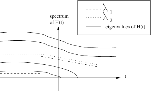
Defining is a somewhat more delicate problem. We would like to exclude the solutions which lie in the unstable manifold of , since they cannot lie in the space of heteroclines from . We do this by separating the eigenvalues corresponding to the intersection of the unstable manifolds of and from those which lie in the stable manifold of . However, there is an obstruction to this technique. In particular, the eigenvalues of vary with time, and can bifurcate. To avoid this issue, we need some kind of regularity for the eigenvalues to prevent them from bifurcating. We follow Floer [7] in the following way:
Conjecture 7.
There is a generic subset (a Baire subset) of choices for in (1) so that if is a heteroclinic orbit, all of the eigenvalues of are simple.
Numerical evidence, as exhibited in [17] and Section 6 suggests that the above Conjecture is true. When we assume that all of the eigenvalues of are simple, and therefore do not undergo any bifurcations other than passing through zero, we shall say is a heterocline contained in .
Let be in such that
- •
on , and
- •
is not an eigenvalue of for any .
We can do this when . See Figure 2.
Definition 8.
Define the Banach algebra (for ) to be the set of in such that the norm
where is an interval containing zero. Likewise, we can define the spaces in a similar way. That these are Banach spaces follows from the boundedness of the . It is also elementary to see that these are Banach algebras.
We then consider as , where is the linearization of about for . (Again, since and are Banach algebras, is the Frechét derivative of .) For a , consider the restriction of to a map . We rewrite
| (9) |
Likewise, we can define .
We define the positive eigenspaces for the equilibria as well
| (10) |
Note in particular that .
Lemma 9.
If is a heterocline that converges to as , then the operator has a finite dimensional kernel for , and in particular
(The condition is only necessary for the case.)
Proof.
Notice that the first term of (9) has finite dimensional kernel by Lemma 4 and closed image by Theorem 5. The second term of (9) is a compact operator since uniformly. Thus has a finite dimensional kernel. Let and consider the set of Cauchy problems
| (11) |
Standard parabolic theory gives uniqueness of solutions to (11), and that a solution lies in the kernel of , the restriction of to . Therefore .
For the other inequality, modify outside of to get a so that the linearization of about satisfies
- •
is isomorphic to as vector spaces,
- •
, and
- •
.
We can do this for a sufficiently large , since tends uniformly to equilibria. Then the flow of
defines an injective linear map from the timeslice at to the timeslice at . (That is, it gives an injective map from to itself – injectivity being an expression of the uniqueness of solutions.) Each element of the kernel of evidently must have and . Therefore, the injectivity ensures that the intersection of the image under the flow of with the complement of has at least dimension . ∎
Remark 10.
Multiplication by , is not a compact operator, in particular note that .
Theorem 11.
Let be a heterocline of (1) which connects equilibria . There exists a union of finite dimensional submanifolds of which
- •
contains and
- •
consists of heteroclines connecting to .
If , then has dimension , and this is maximal among such submanifolds .
Proof.
Observe that is surjective, since it is easy to show that the formula
is a well defined right inverse of . This involves showing that
converges, where we note that the contour changes with time. As it happens, the computation in [10] goes through with the only change that at , we deflect the contour to the right, rather than the left (as in Figure 1). Since Lemma 9 shows that has finite dimensional kernel, then it follows that is a union of finite dimensional manifolds, with a finite maximal dimension. It is obvious that consists entirely of heteroclinic orbits and contains .
It remains to show that the dimension of is as advertised and maximal. Observe that is a compact perturbation of an operator which is time-translation invariant. This follows from the precise choice of being continous and not intersecting the eigenvalues of . and are both surjective by exactly the same reasoning as for . is injective by using separation of variables as in Lemma 4 (noting that all nontrivial solutions blow up in the norm). Therefore the Fredholm index of , hence is zero. However, this implies that is injective.
Since is bijective, any solution to which decays faster than as ends up growing faster than as , and in particular does not tend to zero. As a result, such a solution cannot be in . This implies that , which with the estimate in Lemma 9 completes the proof. ∎
Remark 12.
Even if (when there exist nonsimple eigenvalues of ), the function can still be constructed. As a result, we always get that the connecting manifold is finite-dimensional.
Corollary 13.
The space of heteroclinic orbits has the structure of a cell complex with finite dimensional cells. This cell complex structure is evidently finite dimensional if there exist only finitely many equilibria for (1).
6. An extended example
Consider the following spectial case of (1)
| (12) |
where the choice of in (1) has been fixed. The bifurcation diagram for the equilibria of (12) can be found in Figure 3. The bifurcation diagram is parametrized by three variables: , , . (Since the equilibrium equation is a second-order ODE, it suffices to specify each solution by its value and first derivative at 0.) Based on the Theorem 5, the number of positive eigenvalues shown in Figure 3 corresponds exactly to the dimension of the unstable manifold of each equilibrium.


6.1. Frontier of the stable manifold
According to Figure 3, when , there is only one equilibrium, . It has empty unstable manifold, though of course it is asymptotically unstable (as is shown in [19]). On the other hand, has an infinite dimensional stable manifold, which is not all of , as a consequence of the asymptotic instability. As a result, its stable manifold has a frontier in (which may not be a boundary in the sense of a manifold with boundary). We are interested in the qualitative behavior of solutions near and along this frontier. We know by Lemma 6 of [18] that if they tend to uniformly on compact subsets, then they do so uniformly. It is enlightening to use a numerical procedure to this end. We start solutions at the following family of initial conditions
| (13) |
Using the Fujita technique (exactly as shown in [19]), we can show that for sufficiently negative , the solution started at will not be eternal. As a result, the family of initial conditions intersects the frontier of the stable manifold of . An approximation to the value of which corresponds to the frontier can be easily found using a binary search. Some typical such solutions are shown in Figure 4, and the approximate value of corresponding to the frontier is


The qualitative behavior shown in Figure 4 indicates that there is some kind of traveling disturbance in the frontier solutions, which seems like a traveling wave. However, such a solution also appears to tend uniformly on compact subsets to , so in fact it converges uniformly. (The uniform convergence is not obvious from the figure, due to the numerical solution being truncated at a finite time.) The leading edge of this disturbance collapses to in finite time for solutions just outside the stable manifold of .
6.2. Flow near equilibria with two-dimensional unstable manifolds
Also of interest is the structure of the flow in the unstable manifold of the “fork arms” which occur at , as they approach the pitchfork bifurcation at . Figure 5 shows a schematic of the flow based on numerical evidence. Of particular interest is the behavior near the boundary marked A. Solutions to the right of the boundary are not eternal solutions – they fail to exist for all . Solutions to the left of A are heteroclinic orbits connecting the equilibrium with an unstable manifold of dimension 2 to the equilibrium with an unstable manifold of dimension zero. A typical such solution is shown in Figure 6.


To examine solutions near the boundary A, we center our attention on the case , which has two equilibria, one of which (call it ) has a 2-dimensional unstable manifold. (This corresponds to the right pane of Figure 5.) If we linearize about , the operator has a pair of simple eigenvalues, as is easily seen in the right pane of Figure 6 at . One of these eigenvalues is smaller, to which is associated the eigenfunction in Figure 7. The eigenfunction is associated to the larger eigenvalue. In Figure 5, corresponds to the horizontal direction, and corresponds to the vertical direction. From the proof of Lemma 4, it is clear that spans the tangent space of the unstable manifold at . Therefore, we specify initial conditions for a numerical solver using
| (14) |

(Taking small allows us to approximate solutions which tend to in backwards time.) Since the perturbations along are quite small, and indeed the eigenvalue associated to is much smaller than that associated to , examining the numerical results of evolving is quite difficult. The behavior along the boundary occurs at a much smaller scale than , yet is crucial in determining the long-time behavior of the solution. To remedy this, the boundary behavior is better emphasized by plotting instead. Figure 8 shows the results of evolving initial conditions (14) for and various values of .

Solutions in Figure 8 show a similar kind of behavior as in the case of the frontier of . There is a traveling front, which moves very slowly in the negative -direction. However, the behavior is quite a bit more delicate. The determining factor in locating the frontier of is the perturbation in a direction roughly like , which has a large eigenvalue. On the other hand, for , Figure 5 indicates that such a direction is not parallel to the boundary of the connecting manifold. (The boundary direction is some linear combination of and , with a numerical value for the angle being roughly 1.114975 radians.) The eigenvalue associated to is roughly ten times smaller, and therefore perturbations in that direction are much more sensitive. Additionally, the action of the flow is therefore primarily in the direction of , which tends to mask effects in other directions. For this reason, it was visually necessary to postprocess the numerical solutions by subtracting from them. Otherwise the presence of the traveling front was unclear.
7. Conclusions
We have shown that the tangent space at an equilibrium splits into a finite dimensional unstable subspace, and infinite dimensional center and stable subspaces. However, it is quite clear by [19] that the center subspace is nonempty and large. Indeed, considering the work of [20], the center and stable subspaces are not closed complements of each other. Additionally, we have given conditions for the space of heteroclinic orbits to have a finite dimensional cell complex structure.
References
- [1] D. G. Aronson and James Serrin. Local behavior of solutions of quasilinear parabolic equations. Arch. Rational Mech. Anal., 25(2):81–122, 1967.
- [2] Richard Blaustein. Kudzu’s invasion into Southern United States life and culture. In J. A. McNeeley, editor, The Great Reshuffling: Human dimensions of invasive species, pages 55–62. The World Conservation Union, 2001.
- [3] Haim Brezis. Semilinear equations in without condition at infinity. Appl. Math. Optim., 12(1):271–282, 1984.
- [4] P. Brunovsky and B. Fiedler. Connecting orbits in scalar reaction diffusion equations II: the complete solution. J. Diff. Eq., 81:106–135, 1989.
- [5] Yihong Du and Li Ma. Logistic type equations on by a squeezing method involving boundary blow-up solutions. J. London Math. Soc., 2(64):107–124, 2001.
- [6] K. Kobayashi et al. On the blowing up problem for semilinear heat equations. J. Math. Soc. Japan, 29:407–424, 1977.
- [7] Andreas Floer. A relative Morse index for the symplectic action. Comm. Pure Appl. Math., 41:393–407, 1988.
- [8] Andreas Floer. The unregularized gradient flow of the symplectic action. Comm. Pure Appl. Math., 41:775–813, 1988.
- [9] Hiroshi Fujita. On the blowing up of solutions of the Cauchy problem for . Tokyo University Faculty of Science Journal, 13:109–124, December 1966.
- [10] Dan Henry. Geometric Theory of Semilinear Parabolic Equations. Springer-Verlag, New York, 1981.
- [11] Jürgen Jost. Partial Differential Equations. Springer, New York, 2007.
- [12] Hansjörg Kielhöfer. Bifurcation theory: An introduction with applications to PDEs. Springer, 2004.
- [13] S. Klainerman. Long-time behavior of solutions to nonlinear evolution equations. Arch. Rat. Mech. Anal., 78:73–98, 1982.
- [14] Mitunobu Kurihara. On a Harnack inequality for nonlinear parabolic equations. Publ. RIMS, Kyoto Univ. Ser. A, 3:211–241, 1967.
- [15] Michael Robinso. Construction of eternal solutions for a semilinear parabolic equation, arxiv:0805.0750. 2008.
- [16] James Robinson. Infinite-dimensional dynamical systems. Cambridge University Press, 2001.
- [17] Michael Robinson. An asymptotic-numerical approach for examining global solutions to an ordinary differential equation, arxiv:0709.4664. 2007.
- [18] Michael Robinson. Classification of connecting solutions of semilinear parabolic equations, arxiv:0709.2705. 2007.
- [19] Michael Robinson. Instability of a parabolic equation with a quadratic nonlinearity, arxiv:0704.3989. 2007.
- [20] Phillipe Souplet and Qi Zhang. Stability for semilinear parabolic equations with decaying potentials in and dynamical approach to the existence of ground states. Ann. I. H. Poincaré, 19(5):683–703, 2002.
- [21] Aizik I. Volpert, Vitaly A. Volpert, and Vladimir A. Volpert. Traveling wave solutions of parabolic systems. American Mathematical Society, Providence, 1994.
- [22] F. B. Weissler. Existence and nonexistence of global solutions for a semilinear heat equation. Israel J. Math, 38:29–40, 1981.
- [23] James Wrkich and Qi Zhang. Solvability conditions for some semi-linear parabolic equations (preprint). 2007.
- [24] Eberhard Zeidler. Nonlinear functional analysis and its applications II/A: Linear monotone operators. Springer-Verlag, New York, 1990.
- [25] Qi Zhang. Semilinear parabolic equations on manifolds and applications to the non-compact Yamabe problem. Electron. J. Differential Equations, 46:1–30, 2000.
- [26] Songmu Zheng. Remarks on global existence for nonlinear parabolic equations. Nonlinear Analysis, 1:107–114, 1986.
- [27] Songmu Zheng. Nonlinear parabolic equations and hyperbolic-parabolic coupled systems. Longman Group, New York, 1995.