Holographic generation of complex fields with spatial light modulators: Application to quantum key distribution

Mark T. Gruneisen Warner A. Miller Raymond C. Dymale Affiliation: Boeing LTS, Inc., PO Box 5670, Albuquerque NM 87185 Ayman M. Sweiti Email: Mark.Gruneisen@kirtland.af.mil, wam@fau.edu

16 May 2007

Abstract

There has been considerable interest recently in the generation of azimuthal phase functions associated with photon orbital angular momentum (OAM) for high-dimensional quantum key distribution (QKD). The generation of secure quantum keys requires not only this pure phase basis, but also additional bases comprised of orthonormal superposition states formed from the pure states. These bases are also known as mutually unbiased bases (MUBs) and include quantum states whose wave functions are modulated in both phase and amplitude. While modulo $2\pi$ optical path control with high-resolution spatial light modulators (SLMs) is well suited to creating the azimuthal phases associated with the pure states, it does not introduce the amplitude modulation associated with the MUB superposition states. Using computer-generated holography (CGH) with the Leith-Upatnieks approach to hologram recording however, both phase and amplitude modulation can be achieved. This paper presents a description of the OAM states of a 3-dimensional MUB system and analyzes the construction of these states via CGH with a phase modulating SLM. The effects of phase holography artifacts on quantum-state generation are quantified and a prescription for avoiding these artifacts by preconditioning the hologram function is presented. Practical effects associated with spatially isolating the first-order diffracted field are also quantified and a demonstration utilizing a liquid crystal SLM is presented.

1 Introduction

With advancements in digital electronics, the principles of holography [1] continue to be utilized for new approaches to imaging and diffractive control of optical fields. In digital holography (DH), an imaging sensor and computer record the hologram and image reconstruction is accomplished via digital processing techniques to present high resolution digital images.[2] In computer-generated holography (CGH), a hologram function can be generated computationally and then displayed via digital printing, photolithography or display-based technologies.[1, 3] A 2006 special issue of Applied Optics presents an overview of recent advances in DH and CGH as applied to microscopy, optical trapping and tweezing, interferometry, data recording, beam shaping, and metrology.[4]

There has been considerable interest recently in the generation of azimuthal phase functions associated with photon orbital angular momentum (OAM) for high-dimensional quantum key distribution (QKD).[5] The complex fields associated with these functions are of the form $\exp(il\theta)$ where $\theta$ is the azimuthal coordinate. The integer $l$ denotes the photon orbital angular momentum in units of Planck’s constant over the range $-\infty<l<\infty$ . While the conventional BB84 protocol for QKD [6] is based upon photon spin angular momentum and utilizes two polarization bases (e.g. the horizontal and diagonal bases), extensions of this protocol to higher dimensions is possible.[7] Whether in two dimensions or higher dimensions, secure transmission of quantum keys is ensured by the use of mutually unbiased bases (MUBs).[8, 9] The states associated with each MUB are equally weighted superpositions of the states associated with the other bases. The measurement of a single photon’s state with an incorrect choice of basis results in an unbiased, or meaningless, probabilistic outcome. Preserving this essential feature of the BB84 protocol while implementing QKD with higher dimensional OAM Hilbert spaces, requires one to generate and discriminate each state in each of the MUBs associated with OAM. These OAM MUB states correspond to optical fields that are modulated in both phase and amplitude.

Recent demonstrations5 of the generation of photon OAM have utilized high-resolution programmable optical path modulators to impart the azimuthal phase dependence of the pure states onto optical wavefronts. For values of $l>1$ , the limited range of these spatial light modulators (SLMs) requires that the optical phase function be introduced modulo $2\pi$ . Assuming monochromatic conditions and adhering to the sign conventions of Goodman [10] wherein a positive optical phase delay introduces a negative phase error, the complex transmittance associated with an optical phase delay function $l\theta$ introduced modulo $2\pi$ can be shown to be [11]-[13]

t(\theta)=\sum_{m=-\infty}^{\infty}sinc\left(1-m\right)e^{iml\theta}

(1)

where $m$ is an integer and the sinc function is used according to the convention $sinc(x)=\sin(\pi x)/\pi x$ . The amplitude diffraction efficiency, given by the sinc function, is spatially uniform and unity for $m=1$ and zero otherwise. While modulo $2\pi$ optical phase control is well suited to creating the azimuthal phases associated with the pure states with high diffraction efficiency, the diffractive optics function is calculated without the benefit of a reference wave to encode amplitude information.

Methods for computing hologram functions that give rise to complex field modulation include both analytic and numerical techniques. Historically, the simplicity of fabricating binary holograms motivated the development of numerical techniques for calculating and optimizing the binary hologram function.[1, 14] Recent developments in SLM technologies allow analytic hologram functions to be displayed in real time with megapixel spatial resolution and $8$ -bit phase resolution. Consequently, analytic expressions for hologram recording functions can be used directly in CGH. The off-axis hologram recording approach introduced by Emmett Leith and Juris Upatnieks [15, 16, 17] defines a useful approach to CGH with SLM technologies providing both phase and amplitude modulation of the diffracted field and allowing separation of the diffracted orders. This approach also allows the hologram transmittance and the complex fields associated with the diffracted orders to be expressed analytically for purpose of analysis.

While photon polarization supports QKD in a $2$ -dimensional Hilbert space, in this paper we present a description of OAM MUBs for a three-dimensional Hilbert space and consider the implications of generating these quantum states via CGH with SLM technology. While our analysis is valid for higher dimensional QKD, we present this next-higher dimensional generalization for clarity. Toward this end, the complex transmittance associated with the Leith-Upatnieks approach to recording thin phase holograms is reviewed and evaluated for the case of holographic generation of a MUB state. Artifacts in the holographically generated complex field are discussed and their effects on a QKD system quantified by calculating the weighted inner product of the holographically generated field with the theoretical MUB field. Through preconditioning the CGH function, these artifacts are eliminated. Finally, a demonstration is presented in which an extended graphics array (XGA) format liquid-crystal-on-silicon (LCOS) SLM is utilized to holographically generate an optical field associated with a three-dimensional OAM MUB state.

2 Mutually Unbiased Bases of OAM States in 3 Dimensions

A 3-dimensional Hilbert space admits a maximum of four MUBs. Each of these bases is, by definition, orthonormal and contains three basis vectors. We may freely choose as one of these bases, designated $MUB_{0}$ , the three pure OAM states corresponding to an angular momentum, $l_{a}=a\hbar$ , $l_{b}=b\hbar$ , and $l_{c}=c\hbar$ , where $a,b,z\in Z$ . To further reinforce the vector nature of these states, we utilize Dirac’s ket notation [18] to provide an abstract description of each of these three basis vectors in this MUB.

MUB_{0}=\left\{|a\rangle,|b\rangle,|c\rangle\right\}

(2)

These three ket vectors are orthogonal, providing $a\neq b\neq c$ , and span the $3$ -dimensional Hilbert space. Any other quantum state $|\psi\rangle$ in this space can be written as a linear superposition of the three basis vectors,

|\psi\rangle=\alpha|a\rangle+\beta|b\rangle+\gamma|c\rangle,

(3)

with $\alpha,\_\beta,\ \gamma\in C$ and

\alpha^{*}\alpha+\beta^{*}\beta+\gamma^{*}\gamma=1

(4)

We require that these states be normalized with inner product

\langle i|j\rangle=\delta_{i,j}\ \ \hbox{for}\ i,\_j\in\left\{a,b,c\right\}

(5)

Consider a second MUB basis in this $3$ -dimensional Hilbert space, $MUB_{1}=\left\{|a_{1}\rangle,|b_{1}\rangle,|c_{1}\rangle\right\}$ . Two characteristic features are needed to define another MUB basis. First, the three vectors in such a basis must be orthonormal and second, any state in $MUB_{1}$ should be equally distributed over the three vectors in $MUB_{0}$ . Hence,

|\langle i|j\rangle|^{2}=\frac{1}{3}\ \ \hbox{for}i,j\in\{a_{1},b_{1},c_{1}\}

(6)

The only four MUB bases in this $3$ -dimensional Hilbert space are shown in Table 1. Note that in Table 1, $z=\exp(i2π/3)$ and we have suppressed the normalizing factor of $1/\sqrt{3}$ in each of the nine MUB states in the last three columns.

$MUB_{0}$	$MUB_{1}$	$MUB_{2}$	$MUB_{3}$
$\|a\rangle$	$\|a_{1}\rangle\propto\|a\rangle+\|b\rangle+\|c\rangle$	$\|a_{2}\rangle\propto\|a\rangle+\|b\rangle+z\|c\rangle$	$\|a_{3}\rangle\propto\|a\rangle+\|b\rangle+z^{2}\|c\rangle$
$\|b\rangle$	$\|b_{1}\rangle\propto\|a\rangle+z\|b\rangle+z^{2}\|c\rangle$	$\|b_{2}\rangle\propto\|a\rangle+z\|b\rangle+\|c\rangle$	$\|b_{3}\rangle\propto\|a\rangle+z\|b\rangle+z\|c\rangle$
$\|c\rangle$	$\|c_{1}\rangle\propto\|a\rangle+z^{2}\|b\rangle+z\|c\rangle$	$\|c_{2}\rangle\propto\|a\rangle+z^{2}\|b\rangle+z^{2}\|c\rangle$	$\|c_{3}\rangle\propto\|a\rangle+z^{2}\|b\rangle+\|c\rangle$

Table 1: Dirac notation description of mutually unbiased bases in 3-dimensional Hilbert space.

Following the Dirac notation, we can provide a configuration-space representation of each of these twelve azimuthal MUB states in terms of a real-valued amplitude function $A(\theta)$ and a real-valued phase function $\Phi(\theta)$ . The $MUB_{0}$ states are purely complex and may be expressed as phase function in the optical plane.

$\displaystyle\langle\theta\|a\rangle$	$\displaystyle=e^{ia\theta}$	(7)
$\displaystyle\langle\theta\|b\rangle$	$\displaystyle=e^{ib\theta}$	(8)
$\displaystyle\langle\theta\|c\rangle$	$\displaystyle=e^{ic\theta}$	(9)

Each of the other nine states in Table 1 is of the form,

|d\rangle=\alpha|a\rangle+\beta|b\rangle+\gamma|c\rangle

(10)

and accordingly,

\langle\theta|d\rangle=A(\theta)e^{-i\Phi(\theta)}

(11)

The corresponding real-valued amplitude and phase functions can be expressed in terms of Eq. 11 as

	$\displaystyle A(\theta)$	$\displaystyle=\sqrt{\langle d\|d\rangle}$			(12)
	$\displaystyle\Phi(\theta)$	$\displaystyle=-\tan{\left(\frac{Im\left(\langle\theta\|d\rangle\right)}{Re\left(\langle\theta\|d\rangle\right)}\right)}.$			(13)

For the purpose of this paper, and without loss of generalization, it is convenient to assign the pure states $|a\rangle$ , $|b\rangle$ and $|c\rangle$ , the quantum numbers $|1\rangle$ , $|0\rangle$ and $|-1\rangle$ , respectively. Furthermore, the analysis that follows will concentrate on CGH generation of one representative MUB state, namely

|c_{3}\rangle=\frac{1}{\sqrt{3}}\left(|1\rangle+e^{-i2\pi/3}|0\rangle+|-1\rangle\right)

(14)

which may be expressed in complex field notation with the following real-valued amplitude and phase,

	$\displaystyle A(\theta)$	$\displaystyle=\frac{1}{\sqrt{3}}\sqrt{1-2\cos{\theta}+4\cos^{2}{\theta}}$			(15)
	$\displaystyle\Phi(\theta)$	$\displaystyle=-\tan^{-1}\left(\frac{\sqrt{3}}{4\cos{(\theta)}-1}\right)$			(16)

3 Complex Field Modulation via Phase Modulation CGH

The off-axis hologram recording approach introduced by Leith and Upatnieks defines a useful approach to complex field modulation by CGH with SLM technology. Introducing the reference wavefront off axis leads to spatial separation of the diffracted orders allowing the first-order diffracted field to be isolated from other diffracted components. The functional dependence of the complex field associated with each diffracted order may be derived explicitly. Fourier series representations of thin phase hologram transmittance are given in the standard references for the case of one-dimensional modulation introduced by two planar wavefronts.[1, 10] In this section, we present the more general form that includes spatial modulation of the recorded field and show that phase modulation holography leads to artifacts in both the amplitude and phase of the holographically generated optical field. Based on analytic expressions for these artifacts, we present a prescription for preconditioning the computer-generated hologram in order to avoid these artifacts in the diffracted field. The wavelength dependences associated with holography are suppressed by assuming monochromatic conditions throughout.

3.1 Two-Dimensional Hologram Recording Function

Let $a(\rho,\theta)$ and $\phi(\rho,\theta)$ represent spatially varying real-valued amplitude and phase functions, respectively, where $\rho$ and $\theta$ are the transverse radial and azimuthal coordinates, respectively. The complex optical field comprising both $a(\rho,\theta)$ and $\phi(\rho,\theta)$ may be written as

E(\rho,\theta)=a(\rho,\theta)e^{i\phi(\rho,\theta)}.

(17)

Similarly, the phase associated with an off-axis reference wavefront of slope $\alpha$ along the Cartesian $y$ direction is $k\,\alpha\,y$ which, in polar coordinates can be written as $kα\rho\sin{\theta}$ , where $k$ is the wave number. Hence, the reference wave $R(\rho,\theta)$ is written as,

R(\rho,\theta)=be^{-ik\alpha\rho\sin{\theta}},

(18)

where $b$ is a constant amplitude. In order to maximize fringe contrast and maintain a monotonic relationship between fringe contrast and amplitude, the reference beam amplitude $b$ is chosen to be equal to the maximum value of the amplitude $a(\rho,\theta)$ denoted $a_{max}$ . The spatially varying intensity associated with the superposition of both fields is

I(\rho,\theta)=a^{2}(\rho,\theta)+a^{2}_{max}+2a(\rho,\theta)a_{max}\cos{(\phi(\rho,\theta)-k\alpha\rho\sin{\theta})}

(19)

. To allow for scaling of the hologram recording function, the computer-generated holography function $f_{cgh}(\rho,\theta)$ is defined as

f_{cgh}\left(\rho,\theta\right)=\sigma\frac{I(\rho,\theta)}{I_{max}},

(20)

where $I_{max}$ normalizes $I(\rho,\theta)$ to unity and the parameter $\sigma$ establishes the maximum value.

In principle, this function can be represented as a thin amplitude hologram via an amplitude modulating SLM or as a thin phase hologram via an optical path modulating SLM. Commercially available optical path modulating SLMs include piston-only micro-mirror arrays [19] based on micro electro-mechanical systems (MEMS) manufacturing and parallel-aligned nematic liquid-crystal (PA-NLC) media when used with linearly polarized light aligned with the NLC director.[20]-[24] The variable birefringence of PA-NLC media also allows them to be used in conjunction with orthogonal polarizers to create amplitude modulation and is utilized in this manner for display applications. It should be noted however that the complex transmittance also includes a parasitic phase modulation term. Marquez et al. [25] have shown that twisted NLC (TNLC) media can be configured with a tandem arrangement of wave plates and polarizers to produce either nearly pure amplitude modulation or nearly pure phase modulation.

3.2 CGH with an Optical Path Modulating SLM

For the case of implementation with an optical path modulating SLM, the specific form of the complex transmittance is determined by the phenomenology of the SLM. In Sec. 5, we will sample and scale the CGH function of Eq. 20 in order to define an $8$ -bit gray scale XGA signal for the SLM driver. The local response of the LC media is such that the refractive index, and correspondingly the optical phase retardance, decreases with increasing intensity as defined by Eq. 20. Therefore, the change in phase retardance introduced by the SLM is,

\Delta\phi_{SLM}(\rho,\theta)=-\sigma\frac{I(\rho,\theta)}{I_{max}}

(21)

where $\sigma$ defines the maximum change in phase introduced by the SLM. The resulting complex transmittance $t(\rho,\theta)$ of the hologram is given by,

t(\rho,\theta)=e^{-i\sigma\frac{I(\rho,\theta)}{I_{max}}}.

(22)

By substituting Eq. 19 into Eq. 22 and applying the Jacobi-Anger formula along with the identity30

J_{m}(-z)=(-1)^{m}J_{m}(z),

the transmittance can be written in terms of the diffracted orders as,

t(\rho,\theta)=e^{-i\frac{\sigma^{\prime}}{2}}\sum_{m=-\infty}^{\infty}(-1)^{m}J_{m}\left(\sigma^{\prime}\frac{a(\rho,\theta)}{a_{max}}\right)e^{\left(im(\phi(\rho,\theta)-k\alpha\rho\sin{\theta})-i\frac{\sigma^{\prime}}{2}\left(\frac{a(\rho,\theta)}{a_{max}}\right)^{2}\right)}

(23)

where $J_{m}$ is the Bessel function of the first kind of order m with the maximum value of the argument given by $\sigma^{\prime}=2\sigma a^{2}_{max}/I_{max}$ . The coefficient to the series is a spatially uniform phase shift. Assuming that the SLM is illuminated with the reference wave of Eq. 18 with amplitude b now taken to be unity, the transmitted optical field is given by the product of Eqs. 18 and 23,

E_{out}\left(\rho,\theta\right)=e^{-i\frac{\sigma^{\prime}}{2}}\sum_{m=-\infty}^{\infty}(-1)^{m}J_{m}\left(\sigma^{\prime}\frac{a(\rho,\theta)}{a_{max}}\right)e^{-i\phi_{m}(\rho,\theta)},

(24)

where the optical phase of the $m$ -th order diffracted component is

\phi_{m}(\rho,\theta)=-m\phi(\rho,\theta)+(m+1)k\alpha\rho\sin{\theta}+\frac{\sigma^{\prime}}{2}\left(\frac{a(\rho,\theta)}{a_{max}}\right)^{2}

(25)

It is evident that the recorded phase $\phi(\rho,\theta)$ is found in the $m=-1$ order. Applying the Bessel function identity $J_{m}(z)=(-1)^{m}J_{m}(z)$ ,[26] the spatially varying amplitude of the $m=-1$ diffracted order may be written as,

a_{-1}(\rho,\theta)=J_{1}\left(\sigma^{\prime}\frac{a(\rho,\theta)}{a_{max}}\right)

(26)

The diffracted amplitude $a_{1}(\rho,\theta)$ is related to the recorded amplitude $a(\rho,\theta)$ through the $J_{1}$ Bessel function leading to nonlinearities in the amplitude of the holographically generated optical field. The spatially varying efficiency with which optical power is diffracted into this order is given by the square of $a_{1}(\rho,\theta)$ ,

\eta_{-1}(\rho,\theta)=J_{1}^{2}\left(\sigma^{\prime}\frac{a(\rho,\theta)}{a_{max}}\right),

(27)

and achieves a maximum value of $33.9\%$ at the peak of the $J_{1}$ Bessel function. If a given value for the amplitude of the diffracted field is to be defined by a unique value of the argument of the Bessel function, then the parameter $\sigma^{\prime}$ should be chosen such that the Bessel function remains monotonic, $\sigma^{\prime}\leq 1.84$ . The upper limit for the maximum intensity $I_{max}$ is $4a^{2}_{max}$ . For this case, $\sigma^{\prime}=\sigma/2$ and the Bessel function will remain monotonic if $\sigma\leq 3.68$ .

The spatially varying phase associated with the $m=-1$ diffracted order, $\phi_{−1}(\rho,\theta)$ , is given by

\phi_{-1}(x,y)=\phi(\rho,\theta)+\frac{\sigma^{\prime}}{2}\left(\frac{a(\rho,\theta)}{a_{max}}\right)^{2}

(28)

While Eq. 28 indicates the desired phase $\phi(\rho,\theta)$ is constructed by the hologram, it also shows the presence of the aberration term $\frac{\sigma^{\prime}}{2}\left(\frac{a(\rho,\theta)}{a_{max}}\right)^{2}$ . This aberration term is proportional to the spatially varying intensity $a^{2}(\rho,\theta)$ and assumes its maximum value when $a(\rho,\theta)=amax$ . For $\sigma^{\prime}=1.84$ , the maximum phase error would be $0.92$ radians or $0.15$ waves, within the classical quarter-wave Rayleigh criteria for diffraction limited performance.[27]

For applications requiring a high degree of fidelity in the holographically generated wavefronts, CGH offers the opportunity to precondition the computed hologram to compensate for both the $J_{1}$ nonlinearity and the phase aberration. In order to generate an optical field with modulated amplitude $A(\rho,\theta)$ it is only necessary to define the CGH amplitude function $a(\rho,\theta)$ such that the amplitude of the $m=-1$ diffracted field satisfies the relationship

a_{-1}(\rho,\theta)=J_{1}\left(\sigma^{\prime}\frac{a(\rho,\theta)}{a_{max}}\right)=cA(\rho,\theta)

(29)

where $c$ is a scaling factor that for a given value of $\sigma^{\prime}$ matches the maximum values of $J_{1}$ and $A(\rho,\theta)$ . Given the preconditioned amplitude function $a(\rho,\theta)$ , it is then possible to define the preconditioned phase function $\phi(\rho,\theta)$ that gives rise to $\Phi(\rho,\theta)$ . This is done by setting $\phi_{−1}(\rho,\theta)$ in Eq. 28 equal to $\Phi(\rho,\theta)$ .

\phi_{-1}(x,y)=\phi(\rho,\theta)+\frac{\sigma^{\prime}}{2}\left(\frac{a(\rho,\theta)}{a_{max}}\right)^{2}=\Phi(\rho,\theta)

(30)

4 Generation of an OAM MUB State via Phase Modulation Holography

The MUB states that we generate using CGH will never exactly represent the theoretical MUB state. In a QKD system, numerous effects will introduce cumulative deviations from the theoretical state. In addition to the artifacts of phase modulation holography described above, these can include optical aberrations within the system including atmospheric aberrations.[28] In this section, we evaluate the effects of phase modulation holography artifacts on the fidelity of a three dimensional MUB state. We also consider the case where the hologram is preconditioned to minimize these artifacts and evaluate additional diffraction effects associated with spatially isolating the first diffracted order.

4.1 Artifacts of phase modulation holography

For the purpose of illustration, consider the $|c_{3}\rangle$ state of the previous section. Recall from Eqs. 15 of Sec. 2 that the amplitude and phase associated with the superposition state may be written as,

	$\displaystyle A(\theta)$	$\displaystyle=\frac{1}{\sqrt{3}}\left(1-2\cos{(\theta)}+4\cos^{2}{(\theta)}\right)^{\frac{1}{2}}$			(31)
	$\displaystyle\Phi(\theta)$	$\displaystyle=-\tan{\left(\frac{\sqrt{3}}{4\cos{(\theta)}-1}\right)}$			(32)

These are shown in gray scale in the first row of Fig. 1 with the amplitude plot normalized to unity and the phase plot in units of radians. Taking the amplitude $a(\rho,\theta)$ and phase $\phi(\rho,\theta)$ in the CGH calculation to be exactly those of the $|c_{3}\rangle$ state, $a(\rho,\theta)=A(\rho,\theta)$ , $amax=Amax$ , and $\phi(\rho,\theta)=\Phi(\rho,\theta)$ , we can evaluate the effect of the phase modulation holography artifacts on the holographically generated $|c_{3}\rangle$ state. Eqns. [22, 24] give the amplitude and phase of the $m=-1$ order diffracted field to be,

	$\displaystyle a_{-1}$	$\displaystyle=J_{1}\left(\sigma^{\prime}\frac{A(\theta)}{A_{max}}\right)$			(33)
	$\displaystyle\phi_{-1}(\theta)$	$\displaystyle=\Phi(\theta)+\frac{\sigma^{\prime}}{2}\left(\frac{A(\theta)}{A_{max}}\right)^{2}$			(34)

Upon substitution from Eqs. 33 the amplitude and phase of the holographically generated field are,

	$\displaystyle a_{-1}$	$\displaystyle=J_{1}\left(\frac{}{}\left(1-2\cos{(\theta)}+4\cos^{2}{(\theta)}\right)^{\frac{1}{2}}\right)$			(35)
	$\displaystyle\phi_{-1}$	$\displaystyle=-\tan{\left(\frac{\sqrt{3}}{4\cos{(\theta)}-1}\right)}+\frac{\sigma^{\prime}}{6A^{2}_{max}}\left(1-2\cos{(\theta)}+4\cos^{2}{(\theta)}\right)$			(36)

The amplitude and phase functions of Eqs. 35 are evaluated for maximum values of the Bessel function argument given by $\sigma^{\prime}=0.610$ , $1.84$ , $3.13$ , and $3.83$ corresponding to the first half-maximum, peak, second half-maximum, and second zero of the Bessel function, respectively. The results are shown in gray scale in the remaining rows of Fig. 1. For the case of $\sigma^{\prime}=0.610$ , the Bessel function is nearly linear and the first-order amplitude is nearly identical to the $|c_{3}\rangle$ state amplitude shown in the first row. For $\sigma^{\prime}=1.84$ , the nonlinear scaling is more significant and the effects become discernable in the amplitude plot. For larger values of $\sigma^{\prime}$ , the non-monotonic nature of $a_{1}(\theta)$ is clearly evident. At these larger values of $\sigma^{\prime}$ , the phase aberration is also discernable in the plots.

Refer to caption — Figure 1: Calculated amplitudes and phases comparing theoretical complex field to that generated by CGH with phase modulation holography for various values of the phase scaling parameter $\sigma^{\prime}$ .

Quantum mechanics provides us with a physically-meaningful metric over the Hilbert space spanned by the apertured OAM quantum states $|l\rangle$ , where $l\in Z$ , that allows us to compare the fidelity, or the angle between ket vectors, of our holographically generated optical MUB states with the theoretical states. In particular, the metric takes the form of an inner product over the ket vectors between our holographically produced MUB state $|\psi_{h}\rangle$ and the theoretical MUB state $|\psi_{t}\rangle$ , each of which can be represented as wave functions in the azimuthal plane $\{\rho,\theta\}$ .

\langle\psi_{t}|\psi_{h}\rangle=\frac{\int_{0}^{a}\int_{0}^{2\pi}\psi^{*}_{t}(\rho,\theta)\psi_{h}(\rho,\theta)\rho d\rho d\theta}{|\psi_{t}|\,|\psi_{h}|}

(37)

Here, $a$ is the aperture radius, and $|\psi|$ is the norm of the wave function similarly defined as,

|\psi|=\sqrt{\int_{0}^{a}\int_{0}^{2\pi}\psi^{*}(\rho,\theta)\psi(\rho,\theta)\rho d\rho d\theta}

(38)

This inner product in the Hilbert space represents the cosine of the angle in Hilbert space between our observed and idealized MUB state but, more importantly, the square of this inner product represents the probability $P$ that our holographically produced MUB state will be measured (by a perfect MUB state detector) in the theoretical state.

P=|\langle\psi_{t}|\psi_{h}\rangle|^{2}

(39)

We will examine the dependence of this fidelity measure on 1) the phase parameter $\sigma^{\prime}$ for the theoretically defined first diffracted order and 2) the reference wavefront slope for numerical simulations of generating and spatially isolating the first diffracted order.

Fig. 2 shows the calculated probability function as a function of the parameter $\sigma^{\prime}$ . For sufficiently large values of the tilt $\alpha$ , the maximum intensity $I_{max}$ can be made arbitrarily close to $4A^{2}_{max}$ . For the purpose of Fig. 2, it is sufficient to choose $\alpha$ to correspond to $100$ waves of tilt across the aperture and let the maximum intensity $I_{max}$ be represented by $4a^{2}_{max}$ . The maximum value for the argument of the Bessel function then becomes $\sigma^{\prime}=\sigma/2$ and the peak of $J_{1}$ occurs when $A(\theta)=A_{max}$ and $\sigma^{\prime}=1.84$ or, equivalently, $\sigma=3.68$ . The calculated probabilities for all states within a given MUB are identical. Since the pure states of $MUB_{0}$ have constant amplitude, the phase aberration term of Eqs. 33 results in a constant phase shift. Similarly, the $J_{1}$ Bessel function is evaluated at a single value of the argument thus avoiding nonlinearities in the amplitude response.

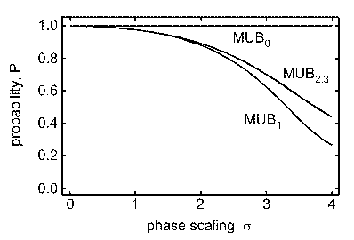
Consequently, the calculated probabilities for $MUB_{0}$ are unity for all values of $\sigma^{\prime}$ . The probabilities associated with the superposition states of the remaining bases all decline with increasing $\sigma^{\prime}$ as shown with the states of $MUB_{2}$ and $MUB_{3}$ falling on the same curve. At $\sigma^{\prime}=1.84$ , the maximum value for which $J_{1}$ remains monotonic, the probability functions have decreased to about $0.90$ . As $\sigma^{\prime}$ increases through the range where $J_{1}$ is no longer monotonic to $\sigma^{\prime}=3.83$ , the second zero of $J_{1}$ , the probability functions decrease further to the vicinity of $0.3$ to $0.5$ with the states in $MUB_{1}$ experiencing the largest reduction.

4.2 Effects of Spatially Isolating the First-Order Diffracted Field

Another practical effect associated with the holographic generation of optical fields is that of isolating the first-order diffracted field from other diffracted orders. In practice, this is accomplished by choosing the angle of the reference wavefront to be sufficiently large that the angular diffraction is greater than the divergence associated with the diffracted fields. The first-order component may then be transmitted by an aperture while blocking the other components.

The effects of spatially isolating the holographically generated $MUB_{3}$ field may also be evaluated numerically. The first row of Fig. 3 again shows the amplitude and phase associated with the theoretical function as defined in Eqs. 31. Note the gray scale for the phase plots is different than that in Fig. 1 in order to remain consistent with the results that follow. The second row shows the numerically calculated holographically generated optical field for the case of a reference wave with $10$ -waves of tilt. In this case, the amplitude and phase artifacts of phase holography have been avoided by using the preconditioned amplitude and phase functions $a(\rho,\theta)$ and $\phi(\rho,\theta)$ as defined in Eqs. 29,30 to calculate the CGH function of Eq. 20. The parameter $\sigma^{\prime}$ is taken to be $1.72$ in order that the Bessel function may be approximated by a polynomial and Eqs. 29,30 may be solved for $a(\rho,\theta)$ and $\phi(\rho,\theta)$ , respectively. The complex transmittance of Eq. 22 is then used to define the optical field transmitted by the hologram as elements of a $768\times 1024$ numerical array. The far-field amplitude is calculated by FFT and is shown in the first column of Fig. 3. The gray scaling has been chosen to be nonlinear to emphasize the $m=\pm 1$ diffracted orders in the figure. A rectangular aperture centered at the $m=-1$ diffracted order is chosen such that the width of the aperture is equal to the order spacing. The field transmitted by the aperture is then transformed by FFT back to the pupil plane. The resulting amplitude and phase are also shown in the second and third column, respectively. Note that while the orders appear to be well resolved, artifacts occur in the amplitude and phase functions. These artifacts may be attributed to interference effects from adjacent orders and diffraction due to the finite aperture size. The third and fourth row show the effects of increasing the reference wave tilt to $50$ and $100$ waves respectively and scaling the aperture size accordingly. Note that the artifacts are significantly reduced.

The fidelity of the holographically generated fields may again be quantified by calculating the probability function in Eq. 39 from numerical data similar to that shown in Fig. 3. The results are shown in Fig. 4 for the case of the $|c_{3}\rangle$ state and are calculated for the cases of $10$ , $30$ , $50$ , $75$ , and $100$ waves of reference wave tilt. The squares represent the case where the CGH function was not preconditioned and therefore include the effects of the amplitude and phase artifacts described in Figs. 1,2. The diamonds represent the case in which the artifacts are precompensated. Fig. 4 shows that the combined effect of preconditioning the hologram and increasing the reference tilt from $10$ to $100$ waves is to increase the inner-product-based probability from $88\%$ to $99.6\%$ .

5 Experimental Demonstration with a LCOS SLM

In this section, we utilize a LCOS SLM to demonstrate holographic generation of the optical field associated with the $|c_{3}\rangle$ quantum state described in the previous sections. The LCOS SLM was developed by Kent State Liquid Crystal Institute and Hana Microdisplay under the Defense Advanced Research Projects Agency (DARPA) Terahertz Operational Reachback (THOR) program.20 The LCOS SLM operates on the principle of discrete-element optical path modulation over a $768\times 1024$ element XGA format. The optical path length of each of the elements may be independently varied over a range of more than $1$ micron corresponding to about two waves of modulation at the $532\,nm$ wavelength used in this demonstration. Prior to using the LCOS SLM in this demonstration, the nonlinearities in the optical phase response were characterized and then utilized in a computer algorithm to linearize the phase response to the CGH function. In addition, interferometric measurements of the SLM surface flatness were utilized to generate a second aberration correction term in the preconditioned CGH phase function $\phi(\rho,\theta)$ . The preconditioned CGH phase function is written as,

\phi(\rho,\theta)=\Phi(\theta)-\frac{\sigma^{\prime}}{2}\left(kW(\rho,\theta)\right)

(40)

where $W(\rho,\theta)$ is the wavefront error associated with the SLM surface flatness and the parameter $\sigma^{\prime}$ is again taken to be $1.72$ . The peak-to-valley magnitude of the SLM wavefront error is $2.15$ waves at $532\,nm$ optical wavelength. With $8$ -bit resolution, the phase response of the SLM spans a range of about $4\pi$ saturating at a gray scale value of $190$ . The approximately $3.44$ radian phase range used in this demonstration is accomplished over about $18$ phase levels. Details of these procedures have been published previously.[20],[21]

The experimental setup is shown in Fig. 5. The output of a $532\,nm$ continuous-wave frequency-doubled Nd:YAG laser is spatially filtered, collimated to approximately $50\,mm$ beam diameter and propagated to the LCOS SLM. The aperture stop defines the area of the SLM utilized to be $1\,cm$ or approximately $90\%$ of the active area. The reflected/diffracted optical field is directed to a one-meter focal length lens to create a far-field plane where another aperture is inserted to spatially select the $m=-1$ order of the hologram. The transmitted order is then propagated to a $250mm$ collimating lens that subsequently creates a re-imaged pupil plane where a camera measures the pupil plane intensity distribution. The optical phase is measured interferometrically by inserting the reference mirror as shown to create a planar reference wavefront and form an interferogram on the camera.

The CGH function of Eq. 20 is calculated using $100$ waves of reference wave tilt and using the phase function $\phi(\rho,\theta)$ in Eq. 40 and the amplitude function $a(\rho,\theta)$ satisfying Eq. 29 with $A(\rho,\theta)$ and $\Phi(\rho,\theta)$ given by the $|c_{3}\rangle$ optical field as given in Eqs. 31. The CGH function is scaled to produce a phase range of $3.44$ radians on the SLM and sampled to define a $768\times 1024$ XGA signal that is sent to the SLM driver. The experimentally generated optical field may be compared to the theoretical $|c_{3}\rangle$ state as follows. The theoretical irradiance function is calculated form the square of the $|c_{3}\rangle$ state amplitude in Eqs. 31. Interferograms associated with the theoretical $|c_{3}\rangle$ optical field are calculated by summing the complex field of Eqs. 31 with a planar reference wavefront and finding the squared modulus. This is done for $10$ waves of interferometer reference tilt in both the vertical and horizontal dimensions as shown in the first row of Fig. 6. The second row of Fig. 6 shows the experimentally measured irradiance and interferograms corresponding to the theoretical case in the first row. The experimental results are in qualitative agreement with the analysis presented in this paper.

6 Conclusions

Computer-generated holography with spatial light modulator technology is evaluated for its utility in generating QKD states based on photon orbital angular momentum. Utilizing azimuthal phase functions to define the orthonormal pure states of a $3$ -dimensional basis, the mutually unbiased bases of a $4$ -bases system are calculated and shown to be azimuthal amplitude and phase functions of the optical field. An analysis of CGH with $2$ -dimensional phase modulators shows that these optical fields may be holographically generated and that artifacts associated with thin phase holography may be compensated in the computation of the hologram. Furthermore, a numerical analysis of practical effects associated with spatially isolating the holographically generated field defines a regime in which the azimuthal field may be constructed with high fidelity. A demonstration with a LCOS SLM shows practical implementation of this approach to generating quantum states for QKD with commercially available technology. Some effects associated with SLM technology, such as pixilation and discretization of phase levels, were not included in the analysis presented here. These details are important in the optimization of SLM designs for implementation of OAM-based QKD.

The authors gratefully acknowledge the important contribution of Prof. Phil Bos, Kent State Liquid Crystal Institute, for his role in both developing and allowing us the use of the LCOS SLM unit described in this work. We also wish to acknowledge important discussions with Glenn Tyler of The Optical Sciences Company and Chris Beetle of Florida Atlantic University. We wish to thank Robert Fugate of the Air Force Research Laboratory and L. N. Durvasula of DARPA for suggesting this research topic. This work was supported by the Air Force Office of Scientific Research.

References

[1] Optical Holography - Principles, Techniques and Applications, P. Hariharan, (Cambridge University Press, Cambridge, 1991).
[2] J. W. Goodman and R. W. Lawrence, “Digital image formation from electronically detected holograms,” Appl. Phys. Lett. 11, 77-79 (1967).
[3] Diffractive Optics for Industrial and Commercial Applications, J. Turunen and F. Wyrowski, Ch. 1.4, pp. 38-45 (Akademie Verlag, Berlin, 1997).
[4] T. C. Poon, T. Yatagai, and W. Juptner, “Digital holography-coherent optics of the 21st century: introduction” and collected papers, App. Opt. 45 special issue on Digital Holography, 821-983 (2006).
[5] Optical Angular Momentum, L. Allen, S. M. Barnett, and M. J. Padgett (IOP Publishing Ltd., London, 2003)
[6] C. H. Bennett and G. Brassard, “Quantum cryptography: public key distribution and coin tossing,” in Proceedings of the IEEE International Conference on Computers, Systems, and Signal Processing, Bangalore, India (IEEE, New York, 1984) 175-179.
[7] N. J. Cerf, A. Karlsson and N. Gisin, “Security of quantum key distribution using d-level systems,” PRL 88, 127902 (2002).
[8] J. Schwinger, “Unitary Operator Bases,” Proc. Nat. Acad. Sci. U.S.A. 46, 560 (1960)
[9] W. K. Wootters and B. D. Fields, ”Optimal state-determination by mutually unbiased measurements,” Ann. Phys. (N. Y.) 191, 363-381 (1989).
[10] Introduction to Fourier Optics, J. W. Goodman (McGraw-Hill, Inc., San Francisco, 1968).
[11] D. A. Buralli, G. M. Morris, and J. R. Rogers, ”Optical performance of holographic kinoforms,” Appl. Opt. 28, 976-983 (1989).
[12] G. J. Swanson, ”Binary optics technology: the theory and design of multi-level diffractive optical elements,” MIT Lincoln Laboratory Tech. Rep. 854, 1-47 (MIT, Cambridge, Mass., 1989).
[13] M. T. Gruneisen, R. C. Dymale, J. R. Rotge, L. F. DeSandre, and D. L. Lubin, ”Wavelength-dependent characteristics of a telescope system with diffractive wavefront control,” Opt. Eng. 44(6) (2005).
[14] M. A. Seldowitz, J. P. Allebach, and D. W. Sweeney, “Synthesis of digital holograms by direct binary search,” App. Opt. 26, 2788-2798 (1987).
[15] E. N. Leith and J. Upatnieks, “Reconstructed wavefronts and communication theory,” J. Opt. Soc. Am 52, 1123-1130 (1962).
[16] E. N. Leith and J. Upatnieks, “Wavefront reconstruction with continuous-tone objects,” J. Opt. Soc. Am 53, 1377-1381 (1963).
[17] E. N. Leith and J. Upatnieks, “Wavefront reconstruction with diffused illumination and three-dimensional objects,” J. Opt. Soc. Am 54, 1295-1301 (1964).
[18] Modern Quantum Mechanics, J. J. Sakurai (Addison-Wesley, Publishing Co., New York, 1994).
[19] A. Gehner, M. Wildenhain, H. Neumann, J. Knobbe, and O. Komenda, “MEMS analog light processing - an enabling technology for adaptive optical phase control,” Proc. SPIE 6113, 61130K 1-15 (2006).
[20] X. Wang, B. Wang, J. Pouch, F. Miranda, M. Fisch, J. E. Anderson, V. Sergan, and P. Bos, ”Liquid crystal on silicon (LCOS) wavefront corrector and beam steerer,” in Advanced Wavefront Control: Methods, Devices, and Applications, J. D. Gonglewski, M. A. Vorontsov, and M. T. Gruneisen, eds., Proc. SPIE 5162, 139-146 (2003).
[21] M. T. Gruneisen, L. F. DeSandre, J. R. Rotge, R. C. Dymale, and D. L. Lubin, ”Programmable diffractive optics for wide-dynamic-range wavefront control using liquid-crystal spatial light modulators,” Opt. Eng. 43, 1387-1393 (2004).
[22] Y. Igasaki, F. Li, N. Yoshida, H. Toyoda, T. Inoue, N. Mukohzaka, Y. Kobayashi, and T. Hara, ”High efficiency electrically-addressable phase-only spatial light modulator,” Opt. Rev. Vol. 6, No. 4, 339-344 (1999).
[23] K. Bauchert, S. Serati, and A. Furman, ”Advances in liquid crystal spatial light modulators,” Optical Pattern Recognition XIII, SPIE Proceedings Vol. 4734, pp. 35 - 43, SPIE Aerosense, Orlando, FL (2002).
[24] $http://www.holoeye.com/phase_{o}nly_{m}odulator_{h}eo1080p.html$
[25] A. Marquez, C. Iemmi, I. Moreno, J. A. Davis, J. Campos, and M. J. Yzuel, “ Quantitative prediction of the modulation behavior of twisted nematic liquid crystal displays based on a simple physical model,” Opt. Eng. 40, 2558-2564 (2001).
[26] Mathematical Handbook for Scientists and Engineers, G. A. Korn and T. M. Korn, Ch. 21.8 (Dover Publications, Inc., Mineola, N.Y., 2000).
[27] W. J. Smith, Modern Optical Engineering (McGraw-Hill, 1966).
[28] C. Paterson, “Atmospheric turbulence and orbital angular momentum of single photons for optical communication,” PRL 94, 153901 (2005).

$MUB_{0}$	$MUB_{1}$	$MUB_{2}$	$MUB_{3}$
$\|a\rangle$	$\|a_{1}\rangle\propto\|a\rangle+\|b\rangle+\|c\rangle$	$\|a_{2}\rangle\propto\|a\rangle+\|b\rangle+z\|c\rangle$	$\|a_{3}\rangle\propto\|a\rangle+\|b\rangle+z^{2}\|c\rangle$
$\|b\rangle$	$\|b_{1}\rangle\propto\|a\rangle+z\|b\rangle+z^{2}\|c\rangle$	$\|b_{2}\rangle\propto\|a\rangle+z\|b\rangle+\|c\rangle$	$\|b_{3}\rangle\propto\|a\rangle+z\|b\rangle+z\|c\rangle$
$\|c\rangle$	$\|c_{1}\rangle\propto\|a\rangle+z^{2}\|b\rangle+z\|c\rangle$	$\|c_{2}\rangle\propto\|a\rangle+z^{2}\|b\rangle+z^{2}\|c\rangle$	$\|c_{3}\rangle\propto\|a\rangle+z^{2}\|b\rangle+\|c\rangle$