Binary-black-hole initial data with nearly-extremal spins

Initial data sets for Einstein’s equations are given on a spatial hypersurface $\Sigma$ and must satisfy the constraint equations

Here, $g_{ij}$ is the induced metric of the slice $\Sigma$, with covariant derivative $\nabla_{i}$, $R:=g^{ij}R_{ij}$ denotes the trace of the Ricci-tensor $R_{ij}$, and $K_{ij}$ denotes the extrinsic curvature of the slice $\Sigma$ as embedded into the space-time manifold ${\cal M}$.

The constraint equations (10) and (11) can be transformed into elliptic partial differential equations using a conformal transformation, e.g. [33]. One introduces a conformal metric, ${\tilde{g}}_{ij}$ via

with the strictly positive conformal factor $\psi>0$. Substituting Eq. (12) into Eq. (10) yields an elliptic equation for $\psi$. One furthermore decomposes the extrinsic curvature into trace and tracefree part,

and splits off a longitudinal part from the tracefree extrinsic curvature,

In Eq. (14), $\sigma$ is a strictly positive weight-function, the longitudinal operator is defined as ${({\mathbb{L}}{V})}^{ij}=2\nabla^{(i}V^{j)}-\frac{2}{3}g^{ij}\nabla_{k}V^{k}$, and $M^{ij}$ is symmetric and trace-free²² 2 It is also possible, but not necessary, to require that $M^{ij}$ is divergence free.. Finally, one introduces the conformally scaled quantities $\sigma=\psi^{6}\tilde{\sigma}$, $M^{ij}=\psi^{-10}\tilde{M}^{ij}$, which allows the momentum constraint [Eq. (11)] to be rewritten completely in terms of conformal quantities:

The Hamiltonian and momentum constraints then become

Given choices for $\tilde{M}^{ij}$, $K$, ${\tilde{g}}_{ij}$ and $\tilde{\sigma}$, and also boundary conditions, one can solve Eqs. (17) and (18) for $\psi$ and $V^{i}$, and then assemble the (constraint-satisfying) initial data $g_{ij}$ and $K^{ij}$.

Many important approaches to construct binary black hole initial data can be cast in this form. The various approaches differ in the choices for the freely specifiable parts and the boundary conditions. Some choices of free data aim for simplicity, such as Bowen-York initial data. Other approaches aim to preserve freedom, resulting in more complicated sets of equations but also more flexibility to control properties of the resulting initial data. The quasi-equilibrium extended-conformal-thin-sandwich approach falls into this second category, and we will exploit precisely its inherent freedom in choosing the free data to construct black holes with nearly-extremal spins.

In this section, we describe two approaches of constructing initial data based on the well-known Bowen-York extrinsic curvature. These two approaches, puncture data and inversion-symmetric data, differ in how they treat the coordinate singularity at $r=0$; both can be obtained from the general procedure outlined in Sec. II.1 by setting $\tilde{\sigma}\equiv 1$, $K\equiv 0$, $\tilde{M}^{ij}\equiv 0$ and by using a conformally flat metric

The momentum constraint [Eq. (18)] then reduces to ${\tilde{\nabla}}\!_{j}(\tilde{\mathbb{L}}{V})^{ij}=0$, which is solved by choosing the analytical Bowen-York solutions [43, 44].

The Bowen-York solutions can be written down most conveniently in Cartesian coordinates, $f_{ij}=\delta_{ij}$:

where $r=(x^{i}x^{j}\delta_{ij})^{1/2}$ is the coordinate distance to the origin and $n^{i}=x^{i}/r$ is the coordinate unit vector pointing from the origin to the point under consideration. The spatially-constant vectors $P^{i}$ and $S^{i}$ parametrize the solutions³³ 3 In Cartesian coordinates, upper and lower indices are equivalent, so index positioning in Eqs. (20)–(23) is unimportant. To find $\tilde{A}^{ij}_{P/S}$ in another coordinate system, first compute the Cartesian components Eqs. (20)–(23), and then apply the desired coordinate transformation.

The conformal factor $\psi$ is then determined by the Hamiltonian constraint [Eq. (17)], which simplifies to

We would like to recover an asymptotically flat space; this implies the boundary condition $\psi\to 1$ as $r\to\infty$.

This boundary condition makes it possible to evaluate the linear ADM-momentum and ADM-like angular momentum of Bowen-York initial data without solving Eq. (24). These quantities are defined by surface integrals at infinity,

where $s^{i}$ is the outward-pointing unit-normal to the integration sphere⁴⁴ 4 At infinity, the normal to the sphere $s^{i}$ is identical to the coordinate radial unit vector $n^{i}$.. By letting $\psi\to 1$ in Eq. (15), one can replace $K_{ij}$ by $\tilde{A}_{ij}$ and then evaluate the resulting integrals. The choice of vector $\xi^{i}$ determines which quantity is computed: For instance, $\xi=\hat{e}_{x}$ corresponds to the x-component of the linear ADM-momentum, $\xi=\partial_{\phi}=-x\hat{e}_{y}+y\hat{e}_{x}$ yields the z-component of the ADM-like angular momentum⁵⁵ 5 As is common in the numerical relativity community, we introduce the phrase “ADM angular momentum” to refer to an angular momentum defined at spatial infinity in the manner of the other conserved ADM quantities of asymptotically flat spacetimes [45], despite the fact that (at least to our knowledge), no such quantity is widely agreed to rigorously exist in general, due to the supertranslation ambiguity that exists in four spacetime dimensions. For recent research on this issue see [46] and references therein. In the present paper, this subtlety can be ignored, because we only compute this quantity in truly axisymmetric spacetimes, with $\vec{\xi}$ the global axisymmetry generator, so that $J_{\rm ADM}$ coincides with the standard Komar integral for angular momentum.. For Eqs. (22) and (23), the results are $P_{\rm ADM}^{i}=P^{i}$ and $J_{\rm ADM}^{i}=S^{i}$, respectively.

The ADM energy is given by the expression

where ${\cal G}_{ij}:=g_{ij}-f_{ij}$, ${\cal G}:={\cal G}_{ij}g^{ij}$. For conformal flatness, Eq. (26) reduces to

The derivative of the conformal factor is known only after Eq. (24) is solved; therefore, in contrast with the linear and angular momenta, $E_{\rm ADM}$ can be computed only after solving the Hamiltonian constraint.

We now turn our attention to inner boundary conditions. $\tilde{A}_{P}^{ij}$ and $\tilde{A}_{S}^{ij}$ are singular at $r=0$. This singularity is interpreted as a second asymptotically flat universe; when solving Eq. (24), this can be incorporated in two ways:

• •

  Inversion Symmetry: The demand that the solution be symmetric under inversion at a sphere with radius $R_{\rm inv}$ centered on the origin [44] results in a boundary condition for $\psi$ at $r=R_{\rm inv}$, namely $\partial\psi/\partial r=-\psi/(2R_{\rm inv})$. The Hamiltonian constraint Eq. (24) is solved only in the exterior of the sphere, $r\geq R_{\rm inv}$, and the solution in the interior can be recovered from inversion symmetry [44], e.g.

  $$\psi\left(x^{i}\right)=\frac{R_{\rm inv}}{r}\psi\left(\frac{R_{\rm inv}^{2}}{r^{2}}x^{i}\right).$$

  (28)

• •

  Puncture data: One demands [24] the appropriate singular behavior of $\psi$ for $r\to 0$ to ensure that the second asymptotically flat end is indeed flat. That is, $\psi$ must behave as

  $$\psi(x^{i})=\frac{m_{p}}{2r}+1+u(x^{i})$$

  (29)

  for some positive parameter $m_{p}$ (the “puncture mass”) and function $u(x^{i})$ that is finite and continuous in $\mathbb{R}^{3}$ and approaches $0$ as $r\to\infty$. Equation (24) then implies an equation for $u$ that is finite everywhere and can be solved without any inner boundaries:

  $${\tilde{\nabla}}\!^{2}u=-\frac{1}{8}\frac{\tilde{A}_{ij}\tilde{A}^{ij}\,r^{7}}{\left(r+\frac{m_{p}}{2}+ur\right)^{7}}.$$

  (30)

  The majority of binary black hole simulations use puncture data, see, e.g., Refs. [9-23].

Both approaches allow specification of multiple black-holes at different locations, each with different spin and momentum parameters $S^{i}$ and $P^{i}$. For puncture data this is almost trivial; this accounts for the popularity of puncture data as initial data for black hole simulations. In contrast, for inversion-symmetric data, one needs to employ a rather cumbersome imaging procedure⁶⁶ 6 Even for a single black hole with $P^{k}\neq 0$, Eq. (22) has to be augmented by additional terms of ${\cal O}(r^{-4})$ to preserve inversion symmetry [44]. (see e.g. [47] for details).

For a single spinning black hole at the origin, the extrinsic curvature $\tilde{A}^{ij}_{S}$ given by Eq. (23) is identical for inversion-symmetric and puncture data. For inversion-symmetric data, the conformal factor has the usual falloff at large radii,

Using Eq. (28) we find the behavior of $\psi$ as $r\to 0$:

Comparison with Eq. (29) shows that this is precisely the desired behavior for puncture data, if one identifies $R_{\rm inv}=m_{p}/2$ and $E/(2R_{\rm inv})=1+u(0)$. Because puncture data has a unique solution, it follows that for single spinning black holes, puncture data and inversion-symmetric data are identical, provided $m_{p}=2R_{\rm inv}$.

For inversion-symmetric initial data for a single, spinning black hole, it is well-known [48] that the apparent horizon coincides with the inversion sphere, $r_{\rm AH}=R_{\rm inv}$. Therefore, we conclude that for puncture data for a single, spinning black hole, the apparent horizon is an exact coordinate sphere with radius $r_{\rm AH}=m_{p}/2$, despite $\tilde{A}^{ij}_{S}$ and $u(x^{i})$ not being spherically symmetric.

Another popular approach of constructing binary-black-hole initial data is the quasi-equilibrium extended-conformal-thin-sandwich (QE-XCTS) formalism [27, 28, 29, 30, 31]. Instead of emphasizing the extrinsic curvature, the conformal thin sandwich formalism [32] emphasizes the spatial metric $g_{ij}$ and its time-derivative. Nevertheless, it is equivalent [33] to the extrinsic curvature decomposition outlined in Sec. II.1. The vector $V^{i}$ is identified with the shift $\beta^{i}$,

and the weight-functions $\sigma$ and $\tilde{\sigma}$ are identified (up to a factor $2$) with the lapse and the conformal lapse, respectively,

The tensor $\tilde{M}_{ij}$ is related to the time-derivative of the spatial metric, $\tilde{u}_{ij}:=\partial_{t}{\tilde{g}}_{ij}$ by

Because $M_{ij}$ is trace free [Eqs. (13) and (15)–(16)], we require $\tilde{u}_{ij}$ to be trace free.

The conformal thin sandwich equations allow control of certain time-derivatives in the subsequent evolution of the constructed initial data. If the lapse $\alpha$ and shift $\beta^{i}$ from the initial data are used in the evolution, for instance, then the trace-free part of $\partial_{t}g_{ij}$ will be proportional to $\tilde{u}_{ij}$. Therefore (see Refs. [30, 27])

The evolution equation for $K$ can be used to derive an elliptic equation for the conformal lapse $\tilde{\alpha}$ (or, equivalently, for $\alpha\psi$). Upon specification of

this fifth elliptic equation is to be solved for $\tilde{\alpha}$ simultaneously with Eqs. (17) and (18), cf. [30, 27].

Our numerical code uses the conformal factor $\psi$, the shift $\beta^{i}$, and the product of lapse and conformal factor $\alpha\psi=\tilde{\alpha}\psi^{7}$ as independent variables, in order to simplify the equation for $\partial_{t}K$. Thus, the actual equations being solved take the form

These equations can be solved only after

1. 1.

   specifying the remaining free data: i.e., the conformal metric ${\tilde{g}}_{ij}$ and the trace of the extrinsic curvature $K$ (we chose already $\tilde{u}_{ij}\equiv 0$ and $\partial_{t}K\equiv 0)$,

2. 2.

   choosing an inner boundary $\mathcal{S}$ which excises the black holes’ singularities, and also an outer boundary $\mathcal{B}$, and

3. 3.

   choosing boundary conditions for $\psi$, $\alpha\psi$, and $\beta^{i}$ on $\mathcal{B}$ and $\mathcal{S}$.

The initial data is required to be asymptotically flat, and the outer boundary $\mathcal{B}$ is placed at infinity⁷⁷ 7 In practice, $\mathcal{B}$ is a sphere with radius $\gtrsim 10^{9}$ times the coordinate radius of the black-hole horizons.. If ${\tilde{g}}_{ij}$ is asymptotically flat, the outer boundary conditions are then

Here $r^{i}$ is the coordinate position vector. The shift boundary condition consists of a rotation (parametrized by the orbital angular velocity $\mathbf{\Omega_{0}}$) and an expansion (parametrized by $\dot{a}_{0}$); the initial radial velocity is necessary for reducing orbital eccentricity in binary-black-hole initial data [49].

The inner boundary condition on the conformal factor $\psi$ ensures that the excision surfaces $\mathcal{S}$ are apparent horizons [27]:

Here $\tilde{s}^{i}:=\psi^{2}s^{i}$, $s^{i}$ is unit vector normal to $\mathcal{S}$, and $\tilde{h}_{ij}:={\tilde{g}}_{ij}-\tilde{s}_{i}\tilde{s}_{j}$ is the induced conformal 2-metric on $\mathcal{S}$.

The inner boundary condition on the shift is

where $\xi^{i}s_{i}=0$. The first term on the right-hand-side ensures that the apparent horizons are initially at rest; the tangential term determines the black hole’s spin [27, 28, 29].

References [27, 28, 29] chose the sign of the last term in Eq. (40) such that positive values of $\Omega_{r}$ counteract the spin of the corotating holes that are obtained with $\Omega_{r}=0$. Here, we are interested in large spins, and we reverse the sign of the last term in Eq. (40) so that positive, increasing $\Omega_{r}$ results in increasing spins.

Two sets of choices for ${\tilde{g}}_{ij}$, $K$, $\mathcal{S}$, and the boundary condition for $\alpha\psi$ on $\mathcal{S}$ are discussed in the next subsections. Each set of choices will be used to construct binary-black-hole initial data in Sec. IV.

As discussed in Sec. II.2, for a single spinning black hole at rest, puncture initial data is identical to inversion-symmetric initial data. Such solutions have been examined in the past (e.g. [48, 63]), and additional results were obtained (partly in parallel to this work) in the study by Dain, Lousto, and Zlochower al [25].

We revisit this topic here to determine the maximum possible spin of Bowen-York (BY) initial data more accurately than before, to establish the power-law coefficients for the approach to these limits with increasing spin parameter $S$, and to present new results about the geometric structure of Bowen-York initial data with very large spin parameter.

We solve Eq. (30) with the pseudo-spectral elliptic solver described in Ref. [64]. The singular point of $u$ at the origin is covered by a small rectangular block extending from $\pm 10^{-4}m_{p}$ along each coordinate axis. This block overlaps four concentric spherical shells with radii of the boundaries at $8\cdot 10^{-5}m_{p},0.005m_{p},0.3m_{p},50m_{p},$ and $10^{9}m_{p}$. The equations are solved at several different resolutions, with the highest resolution using $20^{3}$ basis-functions in the cube, $L=18$ in the spheres and 26 and 19 radial basis-functions in the inner and outer two spherical shells, respectively.

Because of the axisymmetry of the data-set, the rotational Killing vector of the apparent horizon is simply $\partial_{\phi}$. The integral for the quasilocal spin, Eq. (78) turns out to be independent of $\psi$ and can be evaluated analytically with a result equal to the spin-parameter, $S$. Thus we can use this initial data set to check how well our spin-diagnostics and our ADM angular momentum diagnostic works (recall that $J_{\rm ADM}$ is also equal to the spin-parameter $S$). This comparison is performed in Fig. 1, which shows relative differences between the numerically extracted values for the approximate-Killing-vector (AKV) spin, the coordinate spin (defined with the AKV spin in Appendix A), and the ADM angular momentum $J_{\rm ADM}$ relative to the expected answer, $S$. The figure also shows differences between neighboring resolutions for the two quantities of interest below, $S/M^{2}=\chi$ and $S/E_{\rm ADM}^{2}=J_{\rm ADM}/E_{\rm ADM}^{2}=\varepsilon_{J}$.

Figure 1 seems to show exponential convergence with increased resolution $N$. Since puncture data is only $C^{2}$ at the puncture, one would rather expect polynomial convergence. The effect of the non-smoothness at the puncture is mitigated by choosing a very high resolution close to the puncture (a small cube with sides $\pm 10^{-4}m_{p}$ with $20^{3}$ basis-functions). Therefore, for the resolutions considered in Fig. 1, the truncation error is dominated by the solution away from the puncture, and exponential convergence is visible. If we used infinite-precision arithmetic and were pushing toward higher resolution than shown in Fig. 1, then we would expect to eventually see polynomial convergence dominated by the cube covering the puncture.

Next, we construct a series of initial data sets with increasing spin-parameter $S$, and compute $\chi$, $\varepsilon_{J}$, and $\zeta$ for each initial data set. The results are plotted in Fig. 2 and confirm earlier results [63, 26]. In addition, the inset shows that the asymptotic values $\chi_{\rm max}=0.9837$ and $\varepsilon_{u,\rm max}=0.928200$ are approached as power-laws in the spin-parameter,

The exponents of these power-laws are computed here for the first time.

To confirm that the apparent horizon is indeed at $r=R_{\rm inv}$, we ran our apparent horizon finder on the high-spin puncture initial data sets. The horizon finder had great difficulty converging, and the reason for this becomes clear from Fig. 3. The main panel of this figure shows the area of spheres with coordinate radius $r$. The area is minimal at $r=m_{p}/2$, as it must be, since $m_{p}/2=R_{\rm inv}$ is the radius of the inversion sphere. However, the area is almost constant over a wide range in $r$—for $S/m_{p}^{2}=10000$ over about two decades in either direction: $0.01\lesssim r/R_{\rm inv}\lesssim 100$. Thus, the Einstein-Rosen bridge (the throat) connecting the two asymptotically flat universes lengthens as the spin increases, giving rise to an ever-lengthening cylinder. If this were a perfect cylinder, then the expansion would be zero for any $r=\mbox{const}$ cross-section. Because the geometry is not perfectly cylindrical, the expansion vanishes only for $r=m_{p}/2=R_{\rm inv}$, but remains very small even a significant distance away from $r=m_{p}/2=R_{\rm inv}$. This is shown in the inset, which plots the residual of the apparent horizon finder at different radii.

With the lengthening of the throat, the interval in $r$ with small expansion lengthens, and the value of the expansion within this interval reduces. Both effects make it harder for the apparent horizon finder to converge. In Fig. 2, we have used our knowledge of the location of the apparent horizon to set $r_{\rm AH}=m_{p}/2$, rather than to find this surface numerically. Without this knowledge, which arises due to the identification of puncture data and inversion symmetric data, computation of Fig. 2 would have been significantly harder, perhaps impossible.

Let us assume for the moment that the solution $\psi(r)=\frac{m_{p}}{2r}+1+u(r)$ is spherically symmetric (we give numerical evidence below that this is indeed a good approximation). Because $g_{ij}=\psi^{4}f_{ij}$, the area of coordinate spheres is then given by

In the throat region, where $A(r)\approx\mbox{const}$, the conformal factor must therefore behave like $1/\sqrt{r}$, as also argued independently by Dain, Lousto, and Zlochower [25].

To extend on Dain et al.’s analysis, let us substitute Eq. (23) into Eq. (24) to obtain the well-known equation

where $\theta$ is the angle between the spin-direction and the point $x^{i}$. Continuing to assume that $\psi$ is approximately spherically symmetric, we can replace the factor $\sin^{2}\theta$ by its angular average $(4\pi)^{-1}\int\sin^{2}\theta\,d\Omega=2/3$, and obtain

Here, we introduced an overbar $\bar{\psi}$ to distinguish the spherically symmetric solution $\bar{\psi}(r)$ of Eq. (53) from the full solution $\psi(x^{i})$ of puncture/inversion-symmetric initial data. Following Dain et al. [25] we assume that the conformal factor behaves as a power-law ($\bar{\psi}(r)=Ar^{\alpha}$) and substitute this into Eq. (53). We find that Eq. (53) determines the power-law exponent $\alpha=-1/2$ and the overall amplitude $A=(6S^{2})^{1/8}$, so that

In Eq. (54), we chose the scaling $S/m_{p}^{2}$ which is commonly used in the puncture-data literature, but kept $r/R_{\rm inv}$ to emphasize the inversion symmetry of the data in our figures (in a log-plot using $r/R_{\rm inv}$, the solution will appear symmetric, see e.g. Fig. 3). While $\bar{\psi}(r)$ solves the spherically symmetric Eq. (53) exactly, it must deviate from $\psi(x^{i})$ for sufficiently large $r$ because $\bar{\psi}\to 0$ as $r\to\infty$, whereas $\psi\to 1$. The deviation will become significant when $\bar{\psi}\sim 1$, i.e. at radius $r_{x}\sim\sqrt{S/m_{p}^{2}}$. Because of inversion symmetry, this implies a lower bound of validity at $1/r_{x}$, so that Eq. (54) holds for

The circumference of the cylindrical throat is

and its length is

Therefore, the ratio of length to circumference,

grows without bound as $S/m_{p}^{2}$ becomes large, albeit very slowly. The scaling with $(S/m_{p}^{2})^{1/2}$ in Eqs. (55)–(57) might seem somewhat surprising. However, in the large spin limit, $S/M^{2}$ is just a constant close to unity (namely $\chi_{\rm max}=0.9837$). Therefore, $S^{1/2}\approx M$, i.e. the scaling $S^{1/2}$ is effectively merely a scaling with mass.

Figure 4 shows the conformal factor $\psi$, the “puncture function” $u$, and the estimate $\bar{\psi}$ of Eq. (54) for three different values of $S/m_{p}^{2}$. There are several noteworthy features in this figure. First, both $\psi$ and $u$ show clearly three different regimes:

• •

  For large $r$, $\psi\approx 1$ and $u\propto 1/r$. This is the upper asymptotically-flat end.

• •

  For intermediate $r$, $\psi\propto 1/\sqrt{r}$ and $u\propto 1/\sqrt{r}$. This is the cylindrical geometry extending symmetrically around the throat. This region becomes more pronounced as $S$ increases.

• •

  For small $r$, $\psi\propto 1/r$ and $u\approx\mbox{const}$. This is the lower asymptotically-flat end.

Figure 4 also plots the approximate solution $\bar{\psi}$ [cf. Eq. (54)] for its range of validity [given by Eq. (55)]. Note that slope and amplitude of $\bar{\psi}$ fit very well the numerical solution $\psi$. In fact, the agreement is much better than with $u$.

One could also have started the calculation that led to Eq. (54) with Eq. (30). Assuming spherical symmetry, and assuming that $u\gg m_{p}/(2r)+1$, we would have derived Eq. (53), but with $\bar{\psi}$ replaced by $u$. We would then have found the approximate behavior Eq. (54) for $u$. The disadvantage of this approach is the need for additional approximations, which reduce the accuracy of the result. From Fig. 4 we see that, in the throat region, the dotted lines representing $\bar{\psi}$ are close to the dashed lines of $u$. But the agreement between $\psi$ and $\bar{\psi}$ is certainly better.

Finally, we note that the limits of validity of $\bar{\psi}$ [Eq. (55)] match very nicely the points where the numerical $\psi$ diverges from $\bar{\psi}$.

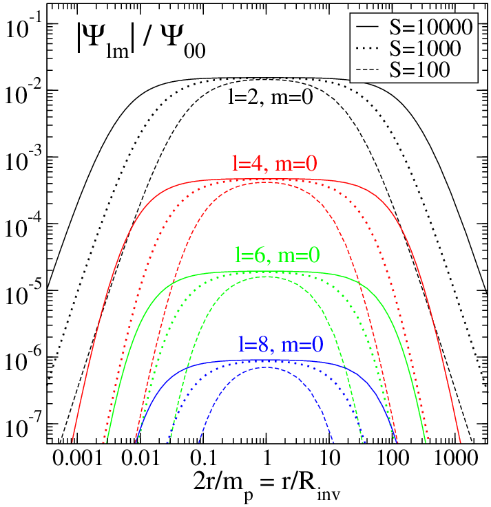
To close this section, we present numerical evidence that indeed $\psi$ is approximately spherically symmetric, the assumption that entered into our derivation of Eq. (54). We decompose the conformal factor of the numerical puncture data solutions into spherical harmonics,

and plot in Fig. 5 the sizes of the $l\neq 0$ modes relative to the spherically symmetric mode $\psi_{00}$. Because of the symmetries of the problem, the only non-zero modes have $m=0$ and even $l$. In the throat region, the largest non-spherically symmetric mode $\psi_{20}$ is about a factor of 65 smaller than the spherically symmetric mode. With increasing $l$, $\psi_{lm}$ decays very rapidly. Also, in both asymptotically flat ends, the non-spherically symmetric modes decay more rapidly than the $l=0$ mode, as expected for asymptotically flat data. This figure again shows nicely the inversion symmetry of the data, under $r/R_{\rm inv}\to(r/R_{\rm inv})^{-1}$. Given the simple structure of the higher modes, it should be possible to extend the analytical analysis of the throat to include the non-spherical contributions. To do so, one would expand $\psi$ as a series in Legendre polynomials in $\theta$; the $\psi^{-7}$-term on the right hand side of Eq. (52) would result in a set of ordinary differential equations for those coefficients. In the throat region, the radial behavior of each mode should be $\propto 1/\sqrt{r}$, and the ordinary differential equations should simplify to algebraic relations.

We have seen in Sec. III.1 that puncture initial data for single, spinning black holes can be constructed for holes with initial spins of $\chi\leq 0.9837$. In this section, we address the analogous question for excision black-hole initial data: how rapid can the initial spin be for a single, spinning black hole constructed using quasiequilibrium, extended-conformal-thin-sandwich (QE-XCTS) initial data?

As noted previously, if the free data ${\tilde{g}}_{ij}$ and $K$ are chosen to agree with the analytic values for a Kerr black hole, $g_{ij}^{\rm Kerr}$ and $K^{\rm Kerr}$, then the QE-XCTS initial data can exactly represent a single Kerr black hole. In this case, $\chi=1$ is obtained trivially by choosing $\tilde{S}=\tilde{M}^{2}=1$, where $\tilde{M}$ and $\tilde{S}$ are the mass and spin, respectively, of the Kerr black hole described by the conformal metric.

Setting aside this trivial solution, we construct conformally-flat, maximally-sliced (CFMS) data for a single, spinning hole. We construct a family of QE-XCTS initial data sets for single spinning black holes by numerically solving the XCTS equations [in the form stated in Eqs. (37a)–(37c)] using the same spectral elliptic solver [64] as in Sec. III.1. The free data are given by Eqs. (41)–(42) and by Eqs. (36a)–(36b).

On the outer boundary $\mathcal{B}$, we impose Eqs. (38a)–(38c). So that the coordinates are asymptotically inertial, we choose $\Omega_{0}=\dot{a}_{0}=0$ in Eq. (38c).

We excise a coordinate sphere of radius $r_{\rm exc}$ about the origin, where

is chosen such that for zero spin $M=1$. On this inner boundary $\mathcal{S}$, we impose Eqs. (39)–(40) and Eq. (44). The spin is determined by Eq. (40): first, the vector $\xi^{i}$ is chosen to be the coordinate rotation vector $\partial_{\phi}$, making the spin point along the positive z axis; then, the rotation parameter $\Omega_{r}$ is varied while the other parameters are held fixed. The spin is measured on the apparent horizon using the approximate-Killing-vector spin (Appendix A); because in this case the space is axisymmetric, the “approximate” Killing vector reduces to the corresponding exact rotational Killing vector.

Figure 6 show how the mass $M$ and AKV spin $S$ depend on $\Omega_{r}$. At $\Omega_{r}=0$, we find the spherically-symmetric solution with $S=0$ and $M_{\text{irr}}=M=1$ (the mass is proportional to the excision radius, and Eq. (60) sets it to unity). Using this spherically-symmetric solution as an initial guess for the elliptic solver, we find solutions for increasing $\Omega_{r}$ with spin increasing initially linearly with $\Omega_{r}$ and with approximately constant mass. Beyond some critical $\Omega_{\rm r,crit}$, the elliptic solver fails to converge, and close to this point, all quantities vary in proportion to $\sqrt{\Omega_{r,{\rm crit}}-\Omega_{r}}$. These symptoms indicate a critical point where the solutions “turn over” and continue towards smaller $\Omega_{r}$. Analogous non-unique solutions of the XCTS equations have been discovered before in Ref. [34]. To construct solutions along the upper branch, one must choose a sufficiently close initial guess for the elliptic solver; we follow the steps outlined in Ref. [34] and are able to find solutions along the upper branch for a wide range of $\Omega_{r}<\Omega_{\rm r,crit}$. As Fig. 6 shows, mass and spin of the horizon in solutions along the upper branch increase with decreasing $\Omega_{r}$, analogous to the findings in [34, 35].

Figure 7 shows the dependence of $\chi=S/M^{2}$, $\varepsilon_{J}=J_{\rm ADM}/E_{\rm ADM}^{2}$, and $\zeta=S/\left(2M_{\text{irr}}^{2}\right)$ on $\Omega_{r}$. The curves reflect again the non-unique solutions. The dimensionless spin $\chi$ increases continuously along the lower branch, and reaches $\chi\approx 0.85$ at the critical point. As $\Omega_{r}$ is decreased along the upper branch, $\chi$ continues to increase, eventually reaching values larger than $0.99$. It appears $\chi$ continues to increase as $\Omega_{r}\to 0$. To find the limiting value, consider that the behavior of the extremality parameter $\zeta$ in the inset of Fig. 7. Assuming that $\zeta$ can be extrapolated to $\Omega_{r}\to 0$, we find a limiting value of $\zeta\approx 0.88$. By Eq. (9), this implies a maximal value of $\chi\approx 0.992$.

References

- [1] M. Volonteri, P. Madau, E. Quataert, and M. J. Rees, Astrophys. J. 620, 69 (2005).
- [2] C. F. Gammie, S. L. Shapiro, and J. C. McKinney, Astrophys. J. 602, 312 (2004).
- [3] S. L. Shapiro, Astrophys. J. 620, 59 (2005).
- [4] J.-M. Wang, Y.-M. Chen, L. C. Ho, and R. J. McLure, Astrophys. J. 642, L111 (2006).
- [5] J. E. McClintock, R. Shafee, R. Narayan, R. A. Remillard, S. W. Davis, and L.-X. Li, Astrophys. J. 652, 518 (2006).
- [6] A. R. King and J. E. Pringle, Monthly Notices of the Royal Astronomical Society: Letters 373, L90 (2006).
- [7] A. R. King, J. E. Pringle, and J. A. Hofmann, Monthly Notices of the Royal Astronomical Society 385, 1621 (2008).
- [8] E. Berti and M. Volonteri (2008), eprint arXiv:0802.0025v2.
- [9] M. Koppitz, D. Pollney, C. Reisswig, L. Rezzolla, J. Thornburg, P. Diener, and E. Schnetter, Phys. Rev. Lett. 99, 041102 (2007), eprint gr-qc/0701163.
- [10] M. Campanelli, C. O. Lousto, Y. Zlochower, and D. Merritt, Phys. Rev. Lett. 98, 231102 (2007a), eprint gr-qc/0702133.
- [11] J. A. Gonzalez, M. D. Hannam, U. Sperhake, B. Brügmann, and S. Husa, Phys. Rev. Lett. 98, 231101 (2007), eprint gr-qc/0702052.
- [12] F. Herrmann, I. Hinder, D. Shoemaker, P. Laguna, and R. A. Matzner, Astrophys. J. 661, 430 (2007a), eprint gr-qc/0701143.
- [13] D.-I. Choi, B. J. Kelly, W. D. Boggs, J. G. Baker, J. Centrella, and J. van Meter, Phys. Rev. D 76, 104026 (2007), eprint gr-qc/0702016.
- [14] M. Campanelli, C. O. Lousto, Y. Zlochower, and D. Merritt, Astrophys. J. Lett. 659, L5 (2007b).
- [15] B. Brügmann, J. A. González, M. Hannam, S. Husa, and U. Sperhake, Phys. Rev. D 77, 124047 (2008), eprint arXiv:0707.0135.
- [16] J. G. Baker, W. D. Boggs, J. Centrella, B. J. Kelly, S. T. McWilliams, M. C. Miller, and J. R. van Meter, Astrophys. J. 668, 1140 (2007), eprint astro-ph/0702390.
- [17] J. D. Schnittman, A. Buonanno, J. R. van Meter, J. G. Baker, W. D. Boggs, J. Centrella, B. J. Kelly, and S. T. McWilliams, Phys. Rev. D 77, 044031 (2008), eprint arXiv:0707.0301v2.
- [18] M. Campanelli, C. O. Lousto, Y. Zlochower, B. Krishnan, and D. Merritt, Phys. Rev. D 75, 064030 (2007c), eprint gr-qc/0612076.
- [19] M. Campanelli, C. O. Lousto, and Y. Zlochower, Phys. Rev. D 74, 084023 (2006a), eprint astro-ph/0608275.
- [20] M. Campanelli, C. O. Lousto, and Y. Zlochower, Phys. Rev. D 74, 041501(R) (2006b), eprint gr-qc/0604012.
- [21] F. Herrmann, I. Hinder, D. M. Shoemaker, P. Laguna, and R. A. Matzner, Phys. Rev. D 76, 084032 (2007b), eprint arXiv:0706.2541v2.
- [22] P. Marronetti, W. Tichy, B. Brügmann, J. González, and U. Sperhake, Phys. Rev. D 77, 064010 (2008).
- [23] E. Berti, V. Cardoso, J. A. Gonzalez, U. Sperhake, and B. Brügmann, Class. Quantum Grav. 25, 114035 (2008), eprint arXiv:0711.1097v2.
- [24] S. Brandt and B. Brügmann, Phys. Rev. Lett. 78, 3606 (1997).
- [25] S. Dain, C. O. Lousto, and Y. Zlochower, Phys. Rev. D 78, 024039 (2008), eprint arXiv:0803.0351v2.
- [26] S. Dain, C. O. Lousto, and R. Takahashi, Phys. Rev. D 65, 104038 (2002).
- [27] G. B. Cook, Phys. Rev. D 65, 084003 (2002).
- [28] G. B. Cook and H. P. Pfeiffer, Phys. Rev. D 70, 104016 (2004).
- [29] M. Caudill, G. B. Cook, J. D. Grigsby, and H. P. Pfeiffer, Phys. Rev. D 74, 064011 (2006), eprint gr-qc/0605053.
- [30] E. Gourgoulhon, P. Grandclément, and S. Bonazzola, Phys. Rev. D 65, 044020 (2002).
- [31] P. Grandclément, E. Gourgoulhon, and S. Bonazzola, Phys. Rev. D 65, 044021 (2002).
- [32] J. W. York, Phys. Rev. Lett. 82, 1350 (1999).
- [33] H. P. Pfeiffer and J. W. York, Phys. Rev. D 67, 044022 (2003).
- [34] H. P. Pfeiffer and J. W. York Jr., Phys. Rev. Lett. 95, 091101 (2005).
- [35] T. W. Baumgarte, N. O’Murchadha, and H. P. Pfeiffer, Phys. Rev. D 75, 044009 (2007).
- [36] D. M. Walsh, Class. Quantum Grav. 24, 1911 (2007), eprint gr-qc/0610129.
- [37] R. A. Matzner, M. F. Huq, and D. Shoemaker, Phys. Rev. D 59, 024015 (1998).
- [38] P. Marronetti and R. A. Matzner, Phys. Rev. Lett. 85, 5500 (2000).
- [39] G. Lovelace, Ph.D. thesis, California Institute of Technology (2007), URL http://etd.caltech.edu/etd/available/etd-05232007-115433.
- [40] K. Taniguchi, T. W. Buamgarte, J. A. Faber, and S. L. Shapiro, Phys. Rev. D 74, 041502(R) (2006).
- [41] G. B. Cook and B. F. Whiting, Phys. Rev. D 76, 041501(R) (2007).
- [42] I. Booth and S. Fairhurst, Phys. Rev. D 77, 084005 (2008), eprint arXiv:0708.2209v3.
- [43] J. M. Bowen, Gen. Relativ. Gravit. 11, 227 (1979).
- [44] J. M. Bowen and J. W. York, Jr., Phys. Rev. D 21, 2047 (1980).
- [45] R. Arnowitt, S. Deser, and C. W. Misner, in Gravitation: An Introduction to Current Research, edited by L. Witten (Wiley, New York, 1962), pp. 227–265, eprint gr-qc/0405109.
- [46] A. Ashtekar, J. Engle, and D. Sloan, Class. Quantum Grav. 25, 095020 (2008).
- [47] G. Cook, Living Rev. Rel. 3 (2000), 5, URL http://www.livingreviews.org/lrr-2000-5.
- [48] J. W. York, Jr. and T. Piran, in Spacetime and Geometry, edited by R. A. Matzner and L. C. Shepley (University of Texas, Austin, 1982), pp. 147–176.
- [49] H. P. Pfeiffer, D. A. Brown, L. E. Kidder, L. Lindblom, G. Lovelace, and M. A. Scheel, Class. Quantum Grav. 24, S59 (2007), eprint gr-qc/0702106.
- [50] M. A. Scheel, H. P. Pfeiffer, L. Lindblom, L. E. Kidder, O. Rinne, and S. A. Teukolsky, Phys. Rev. D 74, 104006 (2006), eprint gr-qc/0607056.
- [51] M. A. Scheel, M. Boyle, T. Chu, L. E. Kidder, K. D. Matthews, H. P. Pfeiffer, and S. A. Teukolsky (2008), in preparation.
- [52] A. Garat and R. H. Price, Phys. Rev. D 61, 124011 (2000).
- [53] J. A. Valiente Kroon, Phys. Rev. Lett. 92, 041101 (2004).
- [54] J. W. York, Jr., in Essays in General Relativity, edited by F. J. Tipler (Academic, New York, 1980), pp. 39–58.
- [55] H. P. Pfeiffer, G. B. Cook, and S. A. Teukolsky, Phys. Rev. D 66, 024047 (2002).
- [56] W. Tichy, B. Brügmann, M. Campanelli, and P. Diener, Phys. Rev. D 67, 064008 (2003).
- [57] S. Nissanke, Phys. Rev. D 73, 124002 (2006).
- [58] N. Yunes, W. Tichy, B. J. Owen, and B. Brügmann, Phys. Rev. D 74, 104011 (2006).
- [59] N. Yunes and W. Tichy, Phys. Rev. D 74, 064013 (2006).
- [60] M. Hannam, S. Husa, B. Brügmann, J. González, and U. Sperhake, Class. Quantum Grav. 24, S15 (2007a).
- [61] B. J. Kelly, W. Tichy, M. Campanelli, and B. F. Whiting, Phys. Rev. D 76, 024008 (2007).
- [62] E. Bonning, P. Marronetti, D. Neilsen, and R. Matzner, Phys. Rev. D 68, 044019 (2003).
- [63] G. B. Cook and J. W. York, Jr., Phys. Rev. D 41, 1077 (1990).
- [64] H. P. Pfeiffer, L. E. Kidder, M. A. Scheel, and S. A. Teukolsky, Comput. Phys. Commun. 152, 253 (2003).
- [65] H. P. Pfeiffer, Ph.D. thesis, Cornell University (2003).
- [66] M. Hannam, S. Husa, B. Brügmann, J. A. Gonzalez, and U. Sperhake, Class. Quantum Grav. 24, S15 (2007b), eprint gr-qc/0612001.
- [67] M. Boyle, D. A. Brown, L. E. Kidder, A. H. Mroué, H. P. Pfeiffer, M. A. Scheel, G. B. Cook, and S. A. Teukolsky, Phys. Rev. D 76, 124038 (2007).
- [68] L. E. Kidder, Phys. Rev. D 52, 821 (1995).
- [69] L. Lindblom, M. A. Scheel, L. E. Kidder, R. Owen, and O. Rinne, Class. Quantum Grav. 23, S447 (2006).
- [70] F. Foucart, L. E. Kidder, H. P. Pfeiffer, and S. A. Teukolsky, Phys. Rev. D 77, 124051 (2008), eprint arXiv:0804.3787.
- [71] J. D. Brown and J. W. York, Phys. Rev. D 47, 1407 (1993).
- [72] A. Ashtekar, C. Beetle, and J. Lewandowski, Phys. Rev. D 64, 044016 (2001), eprint gr-qc/0103026.
- [73] A. Ashtekar and B. Krishnan, Phys. Rev. D 68, 104030 (2003).
- [74] O. Dreyer, B. Krishnan, D. Shoemaker, and E. Schnetter, Phys. Rev. D 67, 024018 (2003).
- [75] E. Schnetter, B. Krishnan, and F. Beyer, Phys. Rev. D 74, 024028 (2006), eprint gr-qc/0604015.
- [76] R. Owen, Ph.D. thesis, California Institute of Technology (2007), URL http://resolver.caltech.edu/CaltechETD:etd-05252007-143511.
- [77] M. Korzynski, Class. Quantum Grav. 24, 5935 (2007).
- [78] URL http://www.netlib.org/lapack.
- [79] E. Anderson, Z. Bai, C. Bischof, S. Blackford, J. Demmel, J. Dongarra, J. DuCroz, A. G. andS. Hammarling, A. McKenney, and D. Sorensen, LAPACK Users’ Guide (Society for Industrial and Applied Mathematics, Philadelphia, 1999).
- [80] P. Anninos, D. Bernstein, S. R. Brandt, D. Hobill, E. Seidel, and L. Smarr, Phys. Rev. D 50, 3801 (1994).
- [81] S. R. Brandt and E. Seidel, Phys. Rev. D 52, 870 (1995).
- [82] M. Alcubierre, B. Brügmann, P. Diener, F. Guzmán, I. Hawke, S. Hawley, F. Herrmann, M. Koppitz, D. Pollney, E. Seidel, et al., Phys. Rev. D 72, 044004 (2005).
- [83] L. Smarr, Phys. Rev. D 7, 289 (1973).
- [84] J. B. Hartle, Phys. Rev. D 9, 2749 (1974).
- [85] J. Massó, E. Seidel, W.-M. Suen, and P. Walker, Phys. Rev. D 59, 064015 (1999).
- [86] S. Carroll, Spacetime and Geometry: An Introduction to General Relativity (Addison Wesley, New York, 2003).