A model of a non-Fermi liquid with symmetry, AF order, and a d-wave SC gap
Abstract
Demanding a consistent quantum field theory description of spin particles near a circular Fermi surface in leads to a unique fermionic theory with relevant quartic interactions which has an emergent Lorentz symmetry and automatically has an internal symmetry. The interacting theory has a low-energy interacting fixed point and is thus a non-Landau/Fermi liquid. Anti-ferromagnetic (AF) and superconducting (SC) order parameters are bilinears in the fields and form the -dimensional vector representation of . An AF phase occurs at low doping which terminates in a first order transition. We incorporate momentum dependent scattering of Cooper pairs near the Fermi surface to 1-loop and derive a new kind of SC gap equation beyond mean field with a d-wave gap solution. Taking into account the renormalization group (RG) scaling properties near the low energy fixed point, we calculate the complete phase diagram as a function of doping, which shows some universal geometric features. The d-wave SC dome terminates on the over-doped side at the fixed point of the RG, which is a quantum critical point. Optimal doping is estimated to occur just below . The critical temperature for SC at optimal doping is set mainly by the universal nodal Fermi velocity and lattice spacing, and is estimated to average around for LSCO. The pseudogap energy scale is identified with the RG scale of the coupling.
I Introduction
In the renormalization group (RG) framework, Landau’s theory of Fermi liquids is characterized by the irrelevance of the interactions of particles near the Fermi surface, in other words the low energy fixed point is simply a free theory of fermions. The underlying reasons for the wide success of Landau/Fermi liquid theory are well-understood[1, 2, 3, 4, 5], and consequently the known models of non-Landau/Fermi liquids are relatively rare. (Henceforth referred to simply as non-Fermi liquids.) An important exception is the Luttinger liquid and other related models consisting of quartic interactions of Dirac fields in spatial dimension. Here the non-Fermi liquid behavior can be attributed to the fact that in , quartic interactions of Dirac fields are marginal operators in the RG sense. In higher dimensions quartic interactions of Dirac fermions are irrelevant and this is one of the reasons why candidate non-Fermi liquid models were not found in the previous works. Whereas more exotic non-Fermi liquid models have been proposed which typically involve gauge fields, the lack of non-Fermi liquid models in appears paradoxical when one considers even the simplest models of itinerant electrons with quartic interactions, such as the Hubbard or t-J model, which are believed to be at strong coupling. Since such models have been proposed as good starting points for thinking about high superconductivity in the cuprates[6, 7, 9], it is certainly worthwhile to continue to try and construct relatively non-exotic models of continuum fermions with quartic interactions that have some resemblance to the Hubbard model and have non-Fermi liquid behavior in the normal state.
Though the search for a novel kind of non-Fermi liquid in provided one of the main initial motivations for the formulation of the model that will be presented and analyzed in this work, the model turns out to have many unexpected bonus features, almost all of which are intrinsic to . We list the most prominent:
The 4-fermion interaction is unique for spin electrons and automatically has symmetry. In the interactions are relevant and the model has a low energy interacting fixed point with non-classical exponents which can be computed perturbatively.
The model generalizes to flavors, where corresponds to spin electrons, and has symmetry. Since this provides a underlying framework based on a microscopic theory for exploring the ideas of Zhang based on [10, 11]. In particular one can derive the effective Ginzburg-Landau theory.
Because of the symmetry the model naturally has both anti-ferromagnetic (AF) and superconducting (SC) order parameters that form the 5-dimensional vector representation of . For repulsive interactions the model has AF order and no SC order in mean field approximation.
When one incorporates momentum dependent scattering to 1-loop to go beyond mean field, an attractive d-wave channel opens up and the momentum dependence of the gap can be calculated. This d-wave SC phase terminates on the over-doped side at the RG fixed point, which is a quantum critical point. Due to mathematical properties of the d-wave gap equation, it also terminates on the under-doped side yielding a “dome”. Due to the properties of the RG flow, this attractive d-wave instability exists for arbitrarily strong repulsive interactions at short distances.
Although the model may be at arbitrarily strong coupling at short distances, the low energy fixed point is at a relatively small coupling , and this renders the model perturbatively calculable. We are thus able to calculate the main features of the complete phase diagram as a function of a doping variable, including the phase boundary of the d-wave superconducting dome and estimate the optimal doping fraction, which is near . This phase diagram depends on a single parameter which encodes the ratio of the strength of the coupling at short versus long distances. In the figure below, we summarize the results of our calculations for , which corresponds to infinite coupling at short distances. The overall scale of temperature is set by the universal nodal Fermi velocity and the lattice spacing.
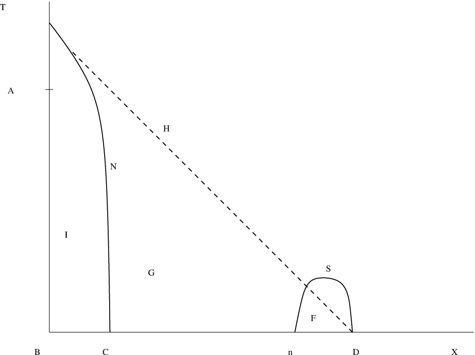
Many of the above properties were highlighted on a list of the most important features of high superconductivity compiled early on in the subject[6, 9]. Because of the importance of the planes, high is believed to be essentially a phenomenon. This, along with the detailed properties of the solution of our model, in particular the phase diagram, led us to propose it as a model of high superconductivity[12]. If our theory turns out to be the correct description, it reveals that the phenomenon of high superconductivity is remarkably universal, with a single energy scale, and its main features follow from the existence of the low energy fixed point in . It is truly a beautiful phenomenon that has managed to realize some subtle theoretical loopholes in the usual requirements of unitarity, the spin-statistics theorem, and the Mermin-Wagner theorem, which are only possible in . Our theory represents a significant departure from the models considered thus far in connection with high , which are reviewed in [13, 14, 16, 15], along with reviews of experimental results. On the other hand, we believe it represents a particular scaling limit of the Hubbard model at and just below half-filling, and is in this sense conservative in comparison with other more exotic ideas, and is thus in line with the early ideas concerning the rôle of AF order and the Heisenberg and Hubbard models[6, 7, 8]. However our model isn’t simply a direct scaling limit of the Hubbard model with no attention paid to the Fermi surface, since the latter only has an symmetry, whereas our theory has the symmetry. In our theory the “fermion sign” problem is solved by doing analytic, perturbative calculations in a fermionic theory from the beginning, and relatively simple 1-loop calculations already reveal the main features.
Irregardless of whether our model has been exactly realized in the laboratory, it can serve as a useful tool for exploring many of the paradigms in the area of strongly correlated electrons and also for developing new methods. For instance, we develop new gap equations that take into account higher order scattering of Cooper pairs near the Fermi surface. Our analysis shows clearly how in one can obtain a momentum dependent gap with a d-wave structure from a rotationally invariant continuum field theory, i.e. without an explicit lattice that breaks the rotational symmetry. This is interesting especially since the precise origin of the d-wave symmetry of the SC gap has been unclear. We also show how to introduce doping in terms of the coupling and RG scale, and a small non-zero temperature as a relativistic mass coupling.
For the remainder of this introduction we outline the organization of the paper and summarize our main results. In section II we motivate the model by showing how it can approximately describe particles and holes near a circular Fermi surface. The manner in which we expand around the Fermi surface is in the same spirit as in [1, 2, 3, 4, 5] but differs in some important ways. For a single spin-less fermion one thereby obtains a free hamiltonian of particles and holes with a massless, i.e. relativistic dispersion relation. In section III we insist on a local quantum field description of the effective theory near the Fermi surface with a consistent quantization. Since the particles are massless, the only known candidate field theories are either Dirac or “symplectic” fermions, which differ primarily by being first versus second order in space-time derivatives respectively. For the remainder of the paper we focus on symplectic fermions since unlike the Dirac fermions, the interactions are relevant. The model was first proposed in this context by one of us[17], where the groundwork was done on the low energy non-Fermi liquid fixed point and in part the AF properties; at the time the SC properties were unknown. As explained in the present paper, the central idea of this previous work, that the AF order parameter is bilinear in symplectic fermion fields and that the low energy RG fixed point describes a quantum critical point, appears to be correct; however as we will see, the quantum critical point terminates the SC rather than AF phase. Quantum critical points in the context of high were emphasized earlier by Vojta and Sachdev[19]. The issue of the unitarity of our theory was mostly resolved in [18] by noting that the hamiltonian is pseudo-hermitian and this is sufficient for a unitary time evolution. In this paper, the expansion around the Fermi surface provides a new view on the pseudo-hermiticity and it is explained how it is related to the kinematics of particles versus holes. The critical exponents were computed to 2-loops in [18], which corrected some errors in[17]. In this paper we analyze many more properties, in particular the AF and d-wave SC ordering properties for the first time.
Since the consistency of the quantization of a fermionic theory with a lagrangian that is second order in time derivatives is at the heart of the unitarity issue, in section IV we work out in detail the dimensional quantum mechanical case where all the subtle consistency issues are present. In this section we also construct the conserved charges for the symmetry. In section V the field theory version in spatial dimensions is defined and spin and charge are identified for the case of . In this section we also define the order parameters for AF and SC order.
In section VI we sketch an argument that the resistivity is linear in temperature in the limit of no interactions. In the next section we consider small thermal perturbations near . By comparing with the specific heat of a degenerate electron gas, we argue that a small non-zero temperature can be incorporated as a coupling in the lagrangian corresponding to relativistic mass and we estimate the constant .
In section VIII the mean field analysis is carried out with potential competition between AF and SC order. As we explain, these two phases actually do not compete in our model in this approximation. As a check of the formalism, we reproduce some of the basic features of the BCS theory for an s-wave gap in the case of an attractive coupling in section IX. For repulsive interactions we find only AF order is possible in mean field approximation and this is studied in section X. There we first argue that this phase must be anti-ferromagnetic by comparing our model with the low energy non-linear sigma model description of the Heisenberg anti-ferromagnet. This gives another motivation for our model at half-filling away from the circular Fermi surface, and explains how the same model can interpolate between a SC phase and an AF one. We argue that the AF phase terminates in a first-order phase transition. The AF gap is then the solution of a transcendental equation that is analyzed in various limits.
In section XI, orbital symmetries of momentum dependent gaps are studied in a model independent way and we explain how a d-wave gap can arise. This analysis is based on a gap equation which is derived in Appendix A. In section XII we compute the 1-loop contributions to the scattering of Cooper pairs and show that at low energies the d-wave channel is attractive if the number of components . Since the theory is free for , this means that only the physically relevant case has d-wave SC. This also means that the d-wave pairing cannot be studied with large methods.
Section XIII is devoted to describing our RG prescription which is specific to . This is necessary for a proper understanding of the phase diagram. In section XIV we present global features of the phase diagram, which is characterized by some universal geometric relations, and bears a striking resemblance to the cuprates. The SC phase terminates at a second order phase transition precisely at the low energy RG fixed point, and is thus a quantum critical point. We also estimate optimal hole doping. In section XV we present detailed numerical solutions to the AF and SC d-wave gap equations at non-zero temperature. For reasonable values of the lattice spacing and universal nodal Fermi velocity, we estimate on average for SC in LSCO. In section XVI we describe the interpretation of the pseudogap within our model.
Although we do not give a complete and rigorous derivation of our model from lattice fermion models, in order to motivate and point out relations, we have collected some known results about the latter in Appendix B.
II Expansion around the Fermi surface
II.1 Kinematics
Let us first ignore spin and consider a single species of fermion described by the free hamiltonian in momentum space
| (1) |
where is the chemical potential, we have defined , and
| (2) |
At finite density and zero temperature, all states with are filled, where the Fermi energy depends on the density, and at zero temperature . The Fermi surface is the manifold of points satisfying .
We wish to consider a band of energies near as shown in Figure 2 for . Let be any wave-vector in such a band, and let denote a ray from the origin to infinity along the direction of . We further assume that the Fermi surface is sufficiently smooth, such that intersects only once. The latter implies that can be uniquely expressed as
| (3) |
where is the vector from the origin to the intersection of with . Whereas the two vectors and are by construction parallel, the vector is either parallel or anti-parallel to . Let us fix to be a small vector parallel to , i.e. pointing radially outward, as shown in Figure 2. Since now is uniquely determined by , we may write . Furthermore, since the particles below the Fermi surface correspond to , the energies near the Fermi surface are approximately given by
| (4) |
where corresponds to above or below the Fermi surface, and
| (5) |
is the Fermi velocity normal to .

Let us now assume that the Fermi surface is rotationally invariant, i.e. depends only on . In the Fermi surface is thus a circle. This leads to the simplification that and are independent of . For any in the band,
| (6) |
where , and . Furthermore, since is normal to , the energies are linear in :
| (7) |
For non-relativistic particles with , .
Since the map from to is one-to-one, we can define the following operators:
| (8) |
where it is implicit that depends on . The above is a canonical transformation, since
| (9) |
After normal ordering, the hamiltonian for the particles in the band is defined to be
| (10) |
where is zero at zero temperature. For the remainder of this paper we mostly set . Since we are only interested in a band of energies near the Fermi surface, we have introduced a cut-off . The vacuum is defined to satisfy . This corresponds to , which correctly implies that all states with are filled. The and thus correspond to particles and holes respectively.
There is an approximation made in obtaining the above hamiltonian having to do with the density of states, and this is crucial to understanding how our expansion differs from previous works. In the rotationally invariant case, for particles above the Fermi surface:
| (11) |
where are angular integrals. Note that due to eq. (6), the angular integrals for and are identical. At least two approximations to the above are meaningful. The first favors low energies where one approximates . This is the approximation that is commonly made in the literature[1, 2]. One the other hand, expanding out the , at high energies the leading term is , and is the most sensitive to the short distance physics and spatial dimensionality. A possible short-coming of the first, low-energy approximation is that the high energy physics is discarded from the beginning. It cannot be recovered by the RG flow to low energies since the latter is irreversible. In the physical problem we are considering, the short-distance physics of the strong Coulomb repulsion is known to be important for understanding the AF phase, so it makes sense to adopt an approximation that favors high energies from the beginning and to then incorporate their effects by an RG flow to lower energies. We thus keep the most important term at short distances and set , i.e. . This is in line with the usual RG idea that it is important to fix the high-energy physics as accurately as possible, and then flow down to lower energies. Finally our choice is necessary for the effective field theory description in the next section. However one should not conclude that every theory with a circular Fermi surface can be described by a relativistic field theory. One signature of a relativistic description is a density of states that is linear in energy: .
The above expansion around the Fermi surface is thus not identical to the expansion in [1, 2, 3, 4, 5], where the integration over is taken to be normal to times the angular integrations, and it is assumed that . This leads to the choice , and the constant is absorbed into the definitions of the operators. Thus in the approach followed in [1, 2, 3, 4, 5], although the angular integrals obviously depend on , the scaling analysis of the dependence leads to marginal 4-fermion interactions for any , and the resulting theory is effectively -dimensional, or a collection of such theories, one for each angular direction. Notably, it was not possible to obtain a non-Fermi liquid based on 4-fermion interactions in this approach[2].
In contrast, in the approach developed in this paper there is a strong dependence on , as in other critical phenomena, and this will turn out to be very important. In particular, it leads to a non-Fermi liquid in . There are other important justifications for this choice. In particular, near half-filling where the interacting lattice model can be mapped to the Heisenberg anti-ferromagnet, there is known to be a relativistic description of the low energy, long wavelength limit in terms of the non-linear sigma model. It will be shown in section X that our choice of field theory near the circular Fermi surface can be extrapolated to half-filling in that an independent derivation of it can be provided exactly at half-filling.
For general processes, physical momentum conservation of the ’s is not equivalent to conservation. However, consider a zero-momentum process proportional to . If the ’s are all exactly on the Fermi surface, then this implies . For even numbers of particles, since all vectors on the Fermi surface have the same length, this is satisfied by pairs of particles with opposite . Allowing now small deviations from the Fermi surface, one has
| (12) |
Because of the particle/hole transformation for the ’s in eq. (8), this is equivalent to overall conservation. Note that by construction, it is not possible for the momentum of a particle and a hole to add up to zero, so in the above -function, holes are paired with other holes, and particles with other particles. Therefore, spatial translational invariance of our local field theory will ensure physical momentum conservation of the ’s for this class of processes.
The important allowed processes are shown in Figure 3. Examples of un-allowed process are shown in Figure 4. The distinction between allowed and un-allowed processes can be made explicit by introducing an operator that distinguishes particles and holes:
| (13) |
where is a unitary operator satisfying so that . An eigenstate with pairs of particles and/or pairs of holes is then required to have . We will return to this in connection with the pseudo-hermiticity of symplectic fermions in the sequel.


II.2 Lattice fermions
In the sequel, our field theory model will be related to lattice models of intinerant electrons such as the Hubbard model, although we do not claim a precise equivalence. The known square lattice model results we will need to make the comparison are all contained in Appendix B. In this section we consider only the free, hopping term. In momentum space the 1-particle energy is (190)
| (14) |
where is the lattice spacing. Equal energy contours in the first Brillouin zone are shown in Figure 5. The Fermi surface at half-filling is the square diamond with corners on the axes. Note that one does not have to be very far below half-filling for the contours to be approximately circular. The free local field theory model in the next section can thus be viewed as an approximate effective theory for free particles on the lattice below half-filling.
An important point is that our model is not simply a direct continuum limit of the lattice model since, without additional care, the latter does not take into account the Fermi surface at finite density. For instance, whereas the Hubbard model has at most an symmetry[36], our continuum model has the larger symmetry. Furthermore, as will be explained in section X, the success of our model can be attributed to the fact that an alternative justification of it can be given right at half-filling so that it can actually interpolate between half-filling and below.

III Requirements on the free local field theory
The main requirements we impose for a local field theory description of the last section are:
(i) The theory has a lagrangian description with a consistent quantization.
(ii) In momentum space the hamiltonian reduces to equation (10) for particles and holes of energy . The latter is a relativistic dispersion relation for massless particles.
In order to motivate our arguments, let us start from non-relativistic particles with . The second-quantized description consists of a single field with lagrangian
| (15) |
The field has the momentum space expansion
| (16) |
Expanding around the Fermi surface one finds
| (17) |
where
| (18) |
We wish to find an effective theory for , which satisfies the relativistic wave equation:
| (19) |
Thus, due to the kinematics of the expansion around the Fermi surface we identify an emergent Lorentz symmetry. In this Lorentz symmetry is . The case of is special in that the Fermi surface consists of only two disconnected points , and the decomposition (17) naturally separates into left and right movers. For higher dimensions there is no such separation since all points on the Fermi surface are related by spatial rotations and continuously connected. There are many additional reasons why is the exceptional case, and these will be pointed out where appropriate in the sequel since some of the literature attempts to draw analogies between and .
There are only two known candidate field theories which differ in whether the lagrangian is first or second order in derivatives. First consider the case of first-order. One then needs to factor the operator into two first-order multiples. The only way to accomplish this is to promote to a multi-component field and introduce a matrix representation , , of the Clifford algebra:
| (20) |
where . One then has
| (21) |
(We have adopted the relativistic notation and , and henceforth, repeated indices are implicitly summed over.) The lagrangian is then the standard first-order Dirac lagrangian:
| (22) |
where . The smallest representation of the Clifford algebra is two dimensional: , and where are the standard Pauli matrices. In this simplest case, although there is a doubling of components, they are constrained by the Dirac equation of motion and the spectrum still consists of one species of particles and holes with hamiltonian eq. (10).
Interactions are relevant to the low energy physics if the operator characterizing them has scaling dimension less than . The classical scaling dimension of the Dirac field is in spatial dimensions, thus a quartic interaction has dimension and is thus only relevant for . It is not even perturbatively renormalizable for . Thus, the Dirac theory should lead to ordinary Landau-Fermi liquid behavior in . It is noteworthy that once again is special, and this helps to explain how for instance the Hubbard model can be mapped onto interacting Dirac fermions, and the low energy fixed point found using special bosonization techniques and spin-charge separation[35]. Simply based on the fact that the interactions in the Hubbard model are strong in , one can rule out a description in terms of Dirac fields with quartic interactions since the latter are irrelevant. Furthermore, it is already understood that one normally needs additional special properties in order to obtain the first-order Dirac theory. For example, it is known to arise when one expands around special nodes (Dirac points) on the Fermi surface for a hexagonal lattice[21], as in graphene, and the multiple components of the Dirac field correspond to different sub-lattices. There is no reason to expect this here for a square lattice, as in the cuprates.
The other candidate field theory is second-order in derivatives, with kinetic term
| (23) |
For fermionic (Grassman) fields, this is a very unconventional theory, since it potentially has problems with the spin-statistics theorem and unitarity; in high energy elementary particle theory it usually corresponds to ghost fields. These issues will be discussed in detail and resolved completely in the next two sections. Here, let us give the main arguments for why this should be the right starting point:
(i) As shown in the next two sections, the free theory in momentum space corresponds precisely to the hamiltonian (10) for particles and holes near a circular Fermi surface. This is of course a perfectly hermitian theory with no negative norm states.
(ii) The fundamental field has scaling dimension and thus quartic interactions have dimension which is actually relevant for . Thus it can have non-Fermi liquid behavior.
(iii) Although we are led to consider this model for the nearly circular Fermi surface below half-filling, a simple argument leads to the same model at half-filling. It is well-known that a low-energy description of excitations above the staggered AF state is described by the non-linear sigma model for a field constrained to have constant length with the action
| (24) |
(See Appendix B.) In our model the anti-ferromagnetic order parameter is bilinear in the fields . The non-linear constraint on the fields follow from imposing a similar constraint on the fields: . This was pointed out in[17]. Inserting this into the above action one finds that one obtains the second order action (23) for the fields up to irrelevant operators (eq. (104) below). Thus the symplectic fermion model with interactions can in principle describe AF order, and in the sequel we will show that this is indeed the case. This is explained in greater detail in section X.
Since only serves to convert dimensions of time and space, it plays the rôle of the speed of light; we can set it to unity since it can always be restored by dimensional analysis. The important point here is that is fixed and universal in our model, in particular it does not depend on the coupling. In the sequel the doping will be related to the coupling, so does not depend on doping either. For high materials, we believe the “speed of light” has actually already been measured[20]. The Fermi surface at half-filling is closest to the nearly circular surface below it in the nodal to direction, so our should correspond to this nodal Fermi velocity. Remarkably, the latter was measured to be universal at low energies, i.e. independent of doping in [20]. Whereas this universality of has not been explained theoretically up to now, it is a necessary aspect of our theory. Taking the slope of the curves in[20] we estimate for LSCO. As we will show in section XV, this gives very reasonable estimates of . Another signature that the system may be in a relativistic regime is a density of states that is linear in energy, as explained in the last section.
IV Symplectic Fermion Quantum Mechanics
As stated above, symplectic fermions are primarily characterized by a lagrangian that is second-order in space and time derivatives. Since this is unfamiliar to most readers and there are some delicate issues in the quantization of such theories, let us first start with the simplest case of quantum mechanics.
IV.1 Canonical quantization
In order to draw comparisons, let us first consider a first order lagrangian as in the Dirac theory:
| (25) |
It is well-understood that this lagrangian has two consistent quantizations, i.e. one can impose either canonical commutation relations or canonical anti-commutation relations . In both cases the hamiltonian is . It’s clear that both options are possible since eq. (15) is a proper second quantized description of either bosons or fermions. For future reference we note that the model has a manifest symmetry.
The second order bosonic version of the above is just the ordinary harmonic oscillator with . Since the first-order lagrangian can be consistently quantized as a fermion or boson, one expects that the second-order case should also be quantizable as a fermion, and as we now describe, this is indeed the case. In order to have a fermionic version, we need at least 2 degrees of freedom since fermionic variables square to zero. Let us therefore consider the lagrangian
| (26) |
where are Grassman variables:
| (27) |
which implies , and we have defined . The canonical momenta are and , which leads to the canonical anti-commutation relations
| (28) |
The canonical hamiltonian is simply
| (29) |
The equation of motion is . Because this is second-order, the mode expansion involves both positive and negative frequencies:
| (30) |
The canonical anti-commutation relations (28) then require
| (31) |
with all other anti-commutators equal to zero. The hamiltonian is
| (32) |
IV.2 Pseudo-hermiticity
The only subtle aspect of the above quantization is the extra minus sign in the expansion of in eq. (30), which was necessary in order to have the canonical relations (31). This minus sign implies that is not the hermitian conjugate of . One can understand this feature more clearly, and also keep track of it, with the operator that distinguishes particles and holes in eq. (13):
| (33) |
In terms of the original variables, the hamiltonian is pseudo-hermitian, . However after using the equations of motion and expressing it in terms of ’s, since it is quadratic in ’s, the hamiltonian (32) is actually hermitian. This issue will be revisited when interactions are introduced in the next section.
IV.3 Symmetries
We now study the symmetries of the -copy theory. Introduce variables , , and define the lagrangian
| (34) |
where is the anti-symmetric matrix . The hamiltonian is
| (35) |
Arrange into a -component vector and consider the transformation , where is a dimensional matrix. Then the lagrangian is invariant if where , and is the transpose. This implies that is an element of the group of dimension . Interestingly, of the classical Lie groups, is the only one that doesn’t play any known rôle in elementary particle physics[25]. Note that the bosonic version of the theory with real components has the symmetry with dimension , thus the fermionic version always has a larger symmetry. The N-component symplectic fermion also has a larger symmetry than the N-component first order fermionic action which has a symmetry or an symmetry if the complex fermions are rewritten in terms of real fields.
The conserved charges that generate the dimensional Lie algebra of are easily constructed. Define
| (36) | |||||
One can easily verify that the hamiltonian commutes with all the charges using
| (37) |
In “momentum” space, the charges are
| (38) | |||||
and they satisfy the hermiticity properties
| (39) |
V Field theory version with spin and interactions
V.1 Lagrangian and Hamiltonian
The field theory version in spatial dimensions follows straightforwardly from the above case with the addition of spatial or momentum integrals. Introducing fields , the action is
| (40) |
and the equations of motion are
| (41) |
The momentum space expansion is
| (42) |
where and . (We do not display the indices since they just correspond to identical copies.) The canonical anti-commutation relations are
| (43) |
which in momentum space leads to
| (44) |
(All other anti-commutators are zero.)
The hamiltonian is
| (45) |
In the limit , we obtain the effective hamiltonian near the Fermi surface in eq. (10), as desired. The mass in this section is an infra-red regulator and is unrelated to the non-relativistic mass above. In section VII we will show that it can be viewed as proportional to the temperature.
The field theory has the same symmetry as the quantum mechanical version. The expressions for the conserved charges are identical to the eqs. (36,38) with additional integrals over or .
There is a unique 4-fermion interaction that preserves the symmetry:
| (46) |
(We have included an overall so that the RG equations below for have no ’s; our convention is the same as in [18].) For , even without imposing the symmetry, there is a unique interaction due to fermionic statistics since there are only independent fields, which implies that higher order terms beyond quartic interactions are zero by Fermi statistics. This interaction is automatically invariant. Positive corresponds to repulsive interactions. Since the field has classical scaling dimension , the interaction is a dimension operator which is relevant for as previously mentioned.
V.2 Pseudo-hermiticity
The symplectic fermion action (40) has a Lorentz invariance if is understood to be a Lorentz scalar. Since is fermionic, to a particle physicist this model would appear to violate the spin-statistics theorem. There are two separate aspects of this issue. First of all, in the condensed-matter context, rotational spin is an internal flavor symmetry (spin fermions corresponds to ) which is not viewed as embedded in the Lorentz group. This implies that spin particles are not forced to be described by the first-order Dirac theory. There is no violation of the spin-statistics connection in our theory since we are quantizing spin particles with fermionic fields. The potential problem rather has to do with unitarity, as explained in the quantum mechanical case studied in the last section, and is manifested in the pseudo-hermiticity property (33). This explains how the proof of the spin-statistics connection is circumvented: the proof assumes that the hamiltonian is built out of fields and their hermitian conjugates and thus doesn’t allow for different fields being related by pseudo-hermitian conjugation[5]. Furthermore, in the end the free hamiltonian in momentum space is a perfectly hermitian theory with no negative norm states.
Whereas the free theory is hermitian in momentum space, for the interacting theory, it follows from (33) that the hamiltonian is pseudo-hermitian:
| (47) |
where the unitary operator and . This sort of generalization of hermiticity was understood to give a consistent quantum mechanics long ago by Pauli[22], and more recently in connection with symmetric quantum mechanics[24, 23]. Let us summarize the main properties enjoyed by pseudo-hermitian hamiltonians:
(i) Define a C-hermitian conjugation as follows:
| (48) |
Then the usual rules are satisfied:
| (49) |
(ii) Define a -conjugate inner product:
| (50) |
Then time-evolution is unitary:
| (51) |
(iii) The eigenvalues of are real:
| (52) |
(iv) Diagonal matrix elements of -pseudo-hermitian operators are real. This will be important in the sequel since it guarantees the reality of vacuum expectation values of pseudo-hermitian order parameters. For our model
| (53) |
In the present work there is a new aspect of the pseudo-hermiticity that relates to the kinematics of the expansion around the Fermi surface. As explained in section II, for the 4-particle processes near the Fermi surface, conservation of relative to the Fermi surface is equivalent to conservation of the physical momentum if particles are paired with particles and holes with holes. Since for particles versus holes, on physical grounds we should restrict to eigenstates with even numbers of holes and even numbers of particles with . Let denote an eigenstate of which is also an eigenstate of . Then . Thus for the eigenstates of interest, .
V.3 Charge and Spin
In order to describe spin electrons, as usual we treat the spin as a flavor and thus consider the theory. The symmetry of the free theory is . A subgroup of this large (10-dimensional) symmetry can be identified with rotational spin and charge.
It was pointed out in [18] that there are potentially two ways to identify electronic spin, and the focus in that work was the subalgebra that exists for all and acts on the indices of . It turns out that the other identification is more natural in the present context since, as explained in section II, the two components corresponding to the indices are already necessary for the expansion of a single spinless fermion near the Fermi surface. There is actually an analog of the identification of spin and charge for arbitrary . Let be an element of the group in the defining dimensional representation. Using the relation
| (54) |
the elements of the Lie algebra satisfy
| (55) |
and a basis is the following: , where are the Pauli matrices, is an dimensional anti-symmetric matrix, and are symmetric matrices[25]. Clearly has an sub-algebra generated by where with the in the -th entry. For this corresponds to an symmetry. However since this sub-algebra does not mix the flavors, it is not the right sub-group for identification with spin as a flavor. The correct identification is the sub-algebra generated by and where now is also traceless. There is also a which commutes with the corresponding to . The is generated by the charges , which form a closed algebra:
| (56) |
The we identify with electric charge is generated by .
Let us now return to the physically interesting case of and label the two components as , corresponding to up and down spins. The spin symmetry is generated by
| (57) | |||||
satisfying the Lie algebra:
| (58) |
(As before .) The charge is generated by
| (59) | |||||
The conserved electric current corresponding to the above charge is
| (60) |
The fields have electric charge . Commutations of the fields with the generators shows that form a doublet whereas is the conjugate:
| (61) |
Note that the above identification is consistent with being particles and holes: whereas . Also, the -particles have whereas the have .
The additional conserved charges with electric charge that complete the Lie algebra are
| (62) | |||||
| (63) |
These symmetries flip the charge and spin of the fields, for instance:
| (64) |
There is no real separation of spin and charge degrees of freedom in our model at this stage, unlike Dirac fermions in , where this separation relies on bosonization. However as we explain in section VIII, the Goldstone bosons are electrically neutral but carry spin quantum numbers.
V.4 order parameters
The 4 fields are in the 4-dimensional spinor representation of . (See e.g. [25]). The important operators are bilinears, which decompose as , where is the singlet , the is the vector representation, and the adjoint. The corresponds to the currents constructed above. The will serve as the order parameters of our model in the sequel. A triplet of fields transforming under the 3-dimensional vector representation of the spin is the following:
| (65) |
where . Note that these fields are electrically neutral. Let us also define two singlets that carry electric charge :
| (66) |
Using the commutation relations of the charges with the -fields, one finds that the 5 order parameters
| (67) |
transform under the 5-dimensional vector representation of . For instance and . The ordering of fermionic operators was chosen such that , more precisely and , which guarantees that vacuum expectation values of are real and those of are complex conjugates. An invariant is the following
| (68) |
Finally the interaction lagrangian density eq. (46) can be expressed as
| (69) |
V.5 Low energy fixed point
The Feynman rules for the theory are the same as for a Lorentz invariant scalar with interaction, which in practice is quite simple[5, 26], except for some all important minus signs. In the sequel we mainly work in euclidean space since this simplifies solving the gap equations and is also appropriate for finite temperature. Where appropriate we will return to real time (Minkowski space) for certain physical quantities. In particular the propagators in euclidean space are
| (70) |
where , and they respect causality. In the usual euclidean conventions the 4-vertex for the interaction in (46) is . (See Figure 9.)
Our RG prescription will be specialized precisely to and is described in detail in section XIII after some 1-loop diagrams are explicitly calculated. In order to obtain a clear physical picture, it will turn out to be important to carry out the RG directly in . However the RG can also be studied perturbatively in an epsilon expansion around . For future reference we summarize the main results obtained in [17, 18] from the epsilon expansion. We will not use these results very much in the sequel; they are included as a guide to the sign and strength of the anomalous corrections to scaling. Since the perturbative expansion differs from that of bosonic scalars only by fermionic minus signs, the standard methods for the bosonic vector models apply. Specifically, these are models of an -vector of scalar fields with interaction . In , the low energy theory is the Wilson-Fisher fixed point[27] describing classical magnets. The anomalous dimensions of the most important operators were computed to 2-loops in [18]. As it turns out, most of the results can be obtained from known results for the models analytically continued to . Besides the field itself and mass term (which will be the thermal perturbation), an additional important class of operators are the bilinears that correspond to order parameters, in particular the of the order parameters when , of the form where is a Pauli matrix. These have no analog that is known to be physically meaningful for the models. It should be emphasized that the quantum critical exponents of our model are completely unrelated to the usual Wilson-Fisher exponents of the bosonic model, since here the vector is a composite bilinear operator and it’s scaling dimension must be calculated in the fundamental -theory.
Let denote the scaling dimension of in inverse length, i.e. energy units. One can also define a correlation length exponent based on the mass :
| (71) |
where :
| (72) |
Specializing the results in [18] to and one obtains
| (73) |
Note that whereas decreases in dimension from the classical value , increases.
Some remarks concerning the case are again appropriate. It is well-known that the low energy fixed points of the bosonic vector models do not extend down to , i.e. . For general this can be viewed as a manifestation of the Mermin-Wagner result[29], which states that spontaneous symmetry breaking in a -dimensional euclidean field theory is not possible in . On the other hand, the models do have a conformally invariant fixed point for in [28]. Since our -component symplectic fermion model is formally equivalent in perturbation theory to , this suggests that our models do not extend to except possibly for . This helps to explain why for instance it has never been considered before in connection with lattice fermion models in .
VI Resistivity in the normal state
In this section we give a rough calculation of the temperature dependence of the conductivity when the interactions are negligible. The rigorous study of this question requires a full finite temperature treatment of the Kubo formula, which is known to be quite subtle, and therefore beyond the scope of the present article. We hope to return to this in a future work, however in this section we present the following non-rigorous scaling argument.
Start with a version of the zero temperature Kubo formula
| (74) |
where are the spatial components of the currents given in (60).
It is well known that the frequency , which corresponds to the DC conductivity, is a delicate limit. Let us first set in the integrand. Using the propagators in eq. (70) one finds
| (75) |
where we have set . The above integral is proportional to . Since the conductivity is dimensionless in , one must have that it is proportional to where is the temperature. For reasons that are unclear, this apparently amounts to setting the overall in eq. (74) equal to . Taking into account the two spin components, and the 4 terms of the above form, one obtains
| (76) |
Therefore the resistivity () is linear in the temperature .
VII Thermal perturbations and anomalous specific heat
The parameters of our model thus far are the Fermi velocity , which we have set equal to , the cut-off , the coupling , and the infra-red regulator mass . The Fermi energy can be viewed as implicit in the cut-off if the latter is taken to be the frequency . The density of the free electron gas is only a function of :
| (77) |
Thus the density can be varied by varying the cut-off, and since is proportional to the cut-off in , equivalently by varying . (See the discussion of the RG in section XIII.)
In this section we suggest how to introduce a small non-zero temperature as the mass . This is similar to how temperature appears in the Landau theory for continuous phase transitions in magnets[30], where there also temperature corresponds to a coupling in an effective action. However there are some important differences, since in the latter the coupling is , whereas here it will be proportional to . Since we have built our model by expanding around the zero temperature Fermi surface, it is not obviously consistent to incorporate a finite temperature by starting over and formulating a finite-temperature version of the fields with Matsubara frequency summations, ignoring that they are effective fields. Rather, since a small non-zero temperature amounts to a small distortion of the Fermi surface, it could correspond to an additional coupling in the lagrangian. If this is correct, then it should be possible to obtain known results in the limit where the interaction is turned off. Suggestive of this possibility is the fact that in natural units the leading contribution to the specific heat of a degenerate electron gas can be expressed entirely in terms of and , i.e. the dependence on the electron mass is only through the Fermi velocity . We emphasize that this way of introducing temperature is expected to be valid for temperatures near zero, and cannot replace a full-fledged finite temperature formalism at arbitrary temperatures. It will however be useful for exploring the temperature dependence of low temperature gaps in the sequel.
In euclidean space, introducing a finite temperature is known to correspond to compactifying the euclidean time to a circle of circumference . Let us consider adding a thermal perturbation to the euclidean action of the form
| (78) |
where is a coupling and is the “thermal operator”. Since the euclidean functional integral is over , the correction to the free energy to lowest order in is . Since the euclidean space-time volume is where is the spatial volume, one finds
| (79) |
This leads us to identify the thermal perturbation with a mass term:
| (80) |
The above relation is consistent with dimensional analysis for a dimensionless parameter. The specific heat at constant volume is . Since the propagator goes as as (See eq. (70) above) one has
| (81) |
where the factor of comes from spin up and down. If the cut-off is equated with the frequency , then this leads to specific heat that is linear in :
| (82) |
(We have re-introduced the Fermi velocity for the sake of comparison.) The above dependence on and is the correct one, i.e. it is the same as for a non-relativistic degenerate electron gas near . Repeating the standard calculation of the specific heat of the electron gas to order (see for instance [30]) for arbitrary , expressing the result in terms of instead of the density, and requiring the result to match eq. (82) fixes the constant :
| (83) |
For , . The case is noteworthy since , and will be commented on below.
The dependence of the specific heat in eq. (82) is a direct consequence of the scaling dimension of , which is twice the scaling dimension of . When one includes the quartic interaction, at the low energy fixed point this scaling dimension has anomalous corrections and this should lead to anomalous dependence of the specific heat. The scaling dimension of was computed perburbatively in an epsilon-expansion [17, 18], and the results summarized in the last section for arbitrary . For , has scaling dimension approximately equal to in the epsilon expansion.
We can provide a naive estimate of the anomalous dependence of the specific heat. Let denote the scaling dimension of . Then if we assume the only effect of the anomalous corrections is to replace by , then since has scaling dimension , this requires . It is not clear that our previous assumption is correct however, since in general could contain terms with . Nevertheless, using our estimate of for the dimension of , this gives . Thus . Though the exponent should perhaps not be taken as very accurate, the general point is that since is shifted downward to from the classical value , this shows that should vanish as . This shift downward is entirely due to a fermionic minus sign[17]. We hope to study this more carefully in future work.
Finally it is important to note that the manner in which we have introduced temperature allows, at least computationally, for phase transitions that break the continuous and symmetries in . The Mermin-Wagner result[29] is the statement that spontaneous symmetry breaking is not possible in a dimensional (space plus time) quantum mechanical system at zero temperature because of infra-red divergences that plague the existence of Goldstone bosons. An example of such a divergence is in eq. (81) for . In the Matsubara approach to finite temperature, time is compactified into a circle of circumference and the discrete Matsubara frequencies are summed over. Thus the arguments of the theorem in principle apply to a finite temperature system in dimensions at each Matsubara frequency. On the other hand, in our model temperature appears as a coupling in the theory, as in classical statistical mechanics in . Furthermore, as discussed in section V, our model breaks down in , since the fixed point is lost, and a manifestation of this is the vanishing of in .
In the sequel, wherever is non-zero, it should be thought of as representing a small non-zero temperature.
VIII Mean field analysis
Because of the symmetry, the interaction term in the lagrangian can be expressed in terms of either the magnetic or electric order parameters:
| (84) |
This implies that magnetic and SC order may in principle compete. In this section we study this in mean field approximation.
Introduce auxiliary fields coupled to the order parameters with the action:
| (85) |
Variations imply
| (86) |
Plugging this back into the action, one finds that the interaction is recovered if
| (87) |
The effective action for the auxiliary fields follows from performing the fermionic gaussian integrals over the fields. Let us pass to euclidean space with the usual prescription , . We will refer to the euclidean coordinates as simply . Then the effective action is defined as
| (88) |
where is the free action for the fields. The result is
| (89) |
where the operator is a differential operator that depends on . For constant and , the can be computed in -dimensional euclidean momentum space since the derivatives are diagonal: . For constant fields it is meaningful to define the effective potential where is the -dimensional volume. At finite temperature for instance where is the usual dimensional volume and the inverse temperature. Using , one obtains
| (90) |
In the basis the anti-symmetric matrix is the following:
| (91) |
Using , one finds
| (92) |
The gap equations follow from setting the variation of with respect to and separately equal to zero. The result is the following for :
| (93) |
There is no simultaneous solution with both and non-zero unless one fine tunes to the invariant point . In fact, there is no true competition between AF and SC order in these equations, and the distinction between and is somewhat fictitious, since for one sign of the coupling there are AF solutions and no SC solutions, and visa-versa if the sign is flipped. We thus consider solutions with either pure SC order () or pure magnetic order (). To further clarify the structure of the gap equation in the sequel, let us separate the spatial and temporal parts of the -dimensional momentum vector as . (This notation is different from that of section II where there was a physical momentum; here and henceforth it is relative to the Fermi surface.) We also restore the mass . For pure SC order one then obtains the gap equation:
| (94) |
where . For pure magnetic order one instead has
| (95) |
It is important to note the asymmetry in the signs of the above SC versus magnetic gap equations, which is ultimately traced to the signs in the invariant (68). Thus, although the model has an symmetry that rotates the SC and magnetic order parameters, the gap equations are not invariant under the exchange of and . This implies that the AF gap is related by symmetry to a conventional s-wave gap obtained when one flips the sign of the coupling, described in the next section.
Let us consider now the implications of Goldstone’s theorem. A non-zero vacuum expectation value in any one direction of the 5-vector preserves an subgroup of . Since , there are potentially 4 Goldstone bosons. One of these is associated to the , and when coupled to the electromagnetic field is eaten up by the Anderson-Higgs mechanism. This leaves a spin-1 triplet of Goldstone bosons associated with the 3-vector , and these are the closest thing to spinons in our model. The effective theory for these modes follows from the above effective potential (92) for . For non-constant fields it contains the kinetic energy term .
IX Conventional s-wave superconductivity in for attractive interactions
It is well understood that a gap that spontaneously breaks the symmetry in the presence of electromagnetic gauge potential automatically has the characteristic electromagnetic properties of a superconductor, i.e. Meissner effect, etc. This precursor to the Higgs mechanism can be understood in the original Ginzburg-Landau theory[31]. A clear explanation of this can be found in Weinberg’s book[5].
We are primarily interested in positive coupling since this corresponds to repulsive interactions. (In the next section we describe how this should correspond to the positive Hubbard model.) However as a check of our formalism thus far, let us consider attractive interactions, i.e. negative , or negative Hubbard, which should reveal the usual s-wave SC instability of the BCS theory. As our analysis shows, symplectic fermions give a proper field theoretic description of conventional s-wave superconductivity which has not been considered before.
As expected there is no s-wave superconductivity for positive since the coupling is negative and the gap equation of the last section has no solutions. For pure SC at negative , equation (87) then implies is positive. Specializing to one should recover some of the basic features of the BCS theory. The gap equation reads
| (96) |
As the cut-off goes to infinity, the divergence can be absorbed into the coupling by defining . This gives the 1-loop correction to the RG beta function: and is consistent with the results in [17, 18]. A more complete RG prescription will be described in section XIII where 1-loop diagrams are computed. Note also that positive is marginally relevant, i.e. increases as the energy is lowered. Since has dimension two, let us define a gap with units of energy. When the cut-off is large compared to the solution to the gap equation is approximately
| (97) |
which is characteristic of the BCS theory, i.e. vanishes as goes to zero, and saturates at the cut-off when goes to infinity. The zero temperature gap as a function of behaves as in Figure 6.

Let us now restore the infra-red regulator mass and confirm the idea that it can be viewed as proportional to the temperature, as long as the latter is close enough to zero. As described in section VII, where in . Restoring the mass, the gap equation now reads in :
| (98) |
When is too large, the RHS can go through zero and change sign, at which point the solution is lost. Numerical solutions of the gap as a function of is shown for several values of in Figure 7.

Let denote the value of where the gap disappears. Then, one expects the critical temperature to be given by a formula of the form
| (99) |
where is the gap at and is a constant of order unity. This is similar to the relation in the BCS theory where . The constant can be estimated numerically and shows a weak dependence on , as Table I shows.
X Anti-ferromagnetic phase (Mott-Hubbard insulator)
X.1 Symplectic fermions from the Hubbard model at half-filling
As stated in the introduction, one cannot derive our model by taking a direct scaling limit of a lattice fermion model like the Hubbard model; this should be clear from the fact that they have different symmetries, i.e. versus . The main reason for this is that one needs to take special care of the Fermi surface in taking such a continuum limit. Nevertheless, we can further motivate our model by comparison with lattice models as follows. Since our model has no explicit lattice, the meaning of the phase can only be understood by comparing with low energy, continuum descriptions of magnetism. It is well-known[32, 35] that excitations above the anti-ferromagnetic Néel state of the Heisenberg model are described by the non-linear sigma-model. The basic facts about lattice models we need for this discussion are collected in Appendix B. Since the field corresponds to our vector of order parameters in eq. (65), let us use that notation.
At half-filling and strong coupling, the Hubbard model can be mapped to the Heisenberg model and the order parameter is constrained to have fixed length . In our model, the magnetic order parameter can be expressed as
| (100) |
where are the Pauli matrices. A fixed length constraint on is equivalent to a similar constraint on the ’s. Using
| (101) |
one can show
| (102) |
where . Therefore if one imposes
| (103) |
for some constant , then . (The is consistent with the propagators in Minkowski space, eq. ().)
At half-filling there is a simple argument that leads to symplectic fermions. Imposing the above half-filling constraints in the lagrangian:
| (104) |
where the additional irrelevant operators can be expressed in terms of dimension current-current interactions . Thus, due to the second-order nature of the non-linear sigma model, one obtains a fermionic theory that is second order in space and time derivatives. Furthermore, let us recall now that we showed in sections II and III how symplectic fermions also arise when one expands around a circular Fermi surface. Since for lattice fermions the nearly circular Fermi surface occurs inside the half-filling diamond, this shows how symplectic fermions can actually extend below half filling. Above half-filling (electron rather than hole doping) the same formalism applies where now one expands around the circular Fermi surface centered on the node .
Relaxing the constraint (103) moves us away from half filling. A meaningful measure of the degree of filling that we will utilize in the sequel is the following. Specializing the formula (81) to in euclidean space and with cut-offs, one finds to zero-th order:
| (105) |
Thus, increasing corresponds to lowering the density below half-filling, so that is a measure of hole doping. We will return to this point when we analyze the phase diagram as a function of doping in section XIV, and will also include 1-loop corrections.
The coupling should be proportional to the Hubbard coupling (See Appendix B). It can be estimated below half-filling near the circular Fermi surface. From the lattice kinetic energy eq. (14), for small , which gives a Fermi velocity . Since has inverse length units, has units of energy. This gives
| (106) |
where is the lattice spacing.
X.2 Solutions of the gap equation
We now study the solutions of the pure AF order gap equation (95) at , which should correspond to zero temperature. Because of the two additional minus signs in the AF gap equation in comparison with the attractive SC one studied in the last section, the interpretation of its solutions is somewhat subtle, and perhaps the most delicate point in this whole paper. First of all, the gap equation definitely has solutions for positive due to the two compensating minus signs. However because of the pole at we require that where is the upper momentum cut-off. A proper understanding of the solutions requires the introduction of both UV and IR cut-offs and to implement the RG directly in . The precise description of our RG prescription is postponed until we calculate some explicit Feynman diagrams and is described in section XIII.
When the equation (87) gives the relation between and and they are both positive. However the resulting relation is purely classical and specific to the auxiliary field construction. Instead we fix the relation between and by requiring consistency with the perturbative RG. To lowest order this requires , in order for eq. (110) to be consistent with eq. (141). The gap equation now reads
| (107) |
Let us define
| (108) |
The result of doing the integral is
| (109) |
Since the -term is positive in the above equation, there are solutions for . In fact, when the coupling is lowered, the term dominates, and the solution approaches and remains there for arbitrarily small . This behavior is not physically sensible since the gap should vanish as the coupling vanishes. To resolve this puzzle, first note that when the gap equation has IR divergences that need to be regulated. Let us therefore introduce a low-energy cut-off . Setting in eq. (107), the result can be written as
| (110) |
The left hand side is precisely an expansion of the running coupling , since by eq. (137), . Denoting the solution as ,
| (111) |
Our interpretation of this value of the coupling is that should vanish for since is a consistent solution at .
The value of the coupling is closely related, but not the same as the low-energy fixed point value of . (See in section XIII.) Namely, at 1-loop the fixed point is at where , thus the low energy fixed point occurs at . As we will see, the low energy quantum critical point at is a second-order continuous phase transition that terminates the super-conducting phase on the over-doped side. This leads us to propose that the termination point of the AF phase is a first-order transition, i.e. the gap drops discontinuously to zero.
Let us return now to solutions of the gap equation with . The solution in the two asymptotic limits have simple expressions. It is useful to use the identity . When , is large. Using , one obtains
| (112) |
As decreases, saturates to since the argument of the must be less than 1 otherwise the solution is complex. Where the solution starts to flatten out can be approximated by extrapolating eq. (112) down to , i.e. around . Using when , one obtains
| (113) |
This behavior is shown in Figure 8 where we have incorporated the drop to zero at .

XI d-wave gap equation in
In the last section we derived gap equations in the approximation that the gap has no momentum dependence. This is essentially equivalent to assuming the lowest order scattering of pairs is momentum independent. In Appendix A we show how to incorporate momentum dependent scattering and derive the following form of gap equation:
| (114) |
where the kernel is given by a Green function related to the scattering of pairs with momenta and . We have set the mass ; it can be restored by . (As explained in Appendix A, is not simply the Fourier transform of .)
For our model the kernel will be computed to 1-loop in the next section. In this section we analyze the orbital properties of the gap in in a model independent way based only on the structure of the gap equation and its symmetries. Similar arguments apply to a BCS type of gap equation.
Let us assume that is symmetric, . If is also rotationally invariant, then its angular dependence arises only through the dependence on . The kernel and gap can thus be expanded as follows:
| (115) |
Substituting the above expansions into the gap equation one sees that due to the non-linearity different can mix. For simplicity consider a single channel, i.e. assume has only one term in its expansion at fixed . The angular integral can be performed and turns out to be independent of :
| (116) |
The result is
| (117) |
It’s important to note that although varies in sign due to the oscillating cosine, the sign of is meaningful and determines whether the channel is attractive or repulsive. Negative corresponds to an attractive channel. Furthermore, any is in principle allowed.
The channel can arise rather naturally from a term in the kernel of the form for a constant, which gives rise to both with the same sign. As we will show in the next section, for our model is the first attractive channel. In particular has the form
| (118) |
with a positive constant which we will calculate in the next section. This leads to a solution of the pure d-wave gap equation of the form
| (119) |
where is a constant satisfying the integral equation:
| (120) |
The dependence on for is of the same form as a particular linear combination of spherical harmonics in , thus we refer to it as , or simply d-wave, as in the literature; can be referred to as and wave.
The above gap equation has some interesting properties, in particular, when is too small. Since this kind of gap equation must be regularized in the UV, we are led to define
| (121) |
where is dimensionless. To estimate the lowest value of with non-zero gap, the integrand in the above equation can be expanded in powers of . Keeping terms of order , one finds that for small it behaves as
| (122) |
where
| (123) |
Thus
| (124) |
For large, one finds
| (125) |
However as we will explain in section XIV, there will also be an upper threshold that comes about when the RG is properly implemented, and this leads to a SC dome.
XII 1-loop scattering and the gap equation kernel
XII.1 Feynman diagrams
In this section we derive the kernel for our model and show that it has an attractive d-wave channel. Let denote the 4-particle vertex function with the overall removed. (Apart from this overall factor, differs from in Appendix A by an overall sign since the Feynman rule vertex is defined to be negative in euclidean space.) The arrows in the figure indicate how the flavor indices are contracted. They also indicate the flow of charge since the interaction is proportional to . This structure is shown in Figure 9, which indicates the interaction of the euclidean space Feynman rules.

The 1-loop contributions to are displayed in Figure 10 and consist of 3 separate channels which differ in how the flavor indices are contracted and also in their momentum dependence. It is interesting to carry out this part of the calculation for arbitrary . The group theory factors are respectively for the three diagrams, where the dependence comes about from the closed loop and a fermionic minus sign.

To this order one thus has
| (126) |
where and is the function:
| (127) | |||||
Since we are interested in low energies, it is meaningful to expand the integrand in powers of . At zero temperature, we can also set . One finds
| (128) |
As explained in Appendix A, the gap equation kernel is obtained by specializing to pairs of opposite momenta. We thus fix
| (129) |
There are also 2 inequivalent ways in which to contract the vertex with external legs which leads us to define
| (130) |
The momentum independent part is the following:
| (131) |
The second term in the above equation can be absorbed into a redefinition of the coupling . It in fact is just the 1-loop contribution to the RG beta-function and we will return to it in section XIII where our RG prescriptions will be fixed.
The order term is
| (132) |
According to the derivation in Appendix A, for static gaps, the kernel in the gap equation is simply with the time components of disregarded, i.e. . This implies that though is closely related to the S-matrix, it is not identical since the external momenta are not on-shell. The above term is then a repulsive correction to the s-wave contribution, which is already repulsive at tree level.
Finally we come to the term:
| (133) |
Using
| (134) |
one sees that this term gives both s and d-wave contributions. Whether the channel is attractive depends on the sign of the factor . For , the above 1-loop s-wave correction is attractive but since the leading tree-level term is repulsive, it is unlikely that it could lead to s-wave pairing. The leading contribution to the d-wave term is attractive for . This is rather interesting since this d-wave instability is invisible to large methods. In the sequel we will make the approximation of the last section and not consider possible mixing of the s and d-wave gaps.
XIII Renormalization group specifically in
In the present context it is most appropriate to adopt the Wilsonian effective action view of the RG. In this approach there are two energy scales to consider, a fixed cut-off scale and a running scale . Integrating out high energy modes leads to couplings that depend on the running scale . Wherever possible, one lets the cut-off go to infinity.
For illustration, consider first the contribution of loop modes with to the momentum-independent part of in :
| (136) |
The effect of these high energy modes is to modify the coupling according to . The beta function is then , in agreement with results in[17, 18]. An equivalent manner to describe this RG prescription is to let and then set the cut-off and keep the dependence on the renormalization energy scale .
Let us now specialize this to . The momentum independent part of G is now the following
| (137) |
where we have sent the cut-off to . This gives , which is consistent with the fact that has units of energy. The latter is an important feature of our model, and in order to deal with it, we define a dimensionless coupling :
| (138) |
The beta function for is now
| (139) |
where the linear term just reflects the classical dimension 1 of . There is a fixed point at
| (140) |
where the above is only approximate due to corrections beyond 1-loop.
The solution to the RG flow equation is then
| (141) |
The fixed point value is reached irregardless of whether the initial coupling at the cut-off is large or small, as long as it is positive. This behavior is sketched in Figure 11.

The coupling that enters the d-wave gap equation can now be expressed as
| (142) |
where we have safely taken to in eq. (135) and set .
XIV Scaling and global features of the phase diagram
XIV.1 RG scaling
For the purposes of comparison with real compounds, our model has only two independent parameters. First is the strength of the coupling at the short distance scale . Second is the overall scale . The complete phase diagram falls into place when one takes into account the RG scaling. Throughout this section it is implicit that we are only working to 1-loop and all equalities should be taken as approximations.
The structure of the phase diagram is most transparent and the universal features more clearly revealed if one works with the dimensionless inverse couplings:
| (143) |
Throughout this section we fix where is the fixed point value. The scale of can now be expressed in a simple way in terms of using eq. (141):
| (144) |
The variable should not be confused with the conventional doping variable in the literature, although it is closely related; the hole doping is the variable below. The above linear relation is specific to and is crucial to understanding the overall structure of the phase diagram. Since the line represents the scale of the coupling, below this line energies are comparable to the coupling and the non-Fermi liquid properties begin to reveal themselves. We have labeled this region the pseudogap as in the literature and will return to it in section XVI. Note that when , .
As we defined them, both the AF and SC gaps and are in units of the cut-off . Since we have performed an RG transformation of the coupling from to , we must also scale the gaps as follows:
| (145) |
It will also be convenient to define the parameter which measures the distance to the fixed point at short distances:
| (146) |
where . The AF gap equation (109) should now be solved for where is replaced by
| (147) |
There are two cases to consider depending on whether the coupling is strong or weak at short distances, i.e. whether is above or below the fixed point value , corresponding to the two curves in Figure 11, which we will refer to as Type A and B.
Type A: strong coupling at short distances
Here we assume , which implies . The scale as a function of now has negative slope
| (148) |
and since the above ratio is by definition less than 1, we have . From eq. (111) the first-order transition that terminates the AF phase corresponds to which translates to
| (149) |
The value is always to the right of since .
Let us turn now to the SC phase. The d-wave gap equation (120) depends on , which by eqns. (121, 142) can be expressed as
| (150) |
The d-wave gap equation only has solutions if is positive, which requires . Furthermore, must be above the threshold by eq. (124). Thus the d-wave SC gap is non-zero in the range
| (151) |
where the lower threshold is a solution to
| (152) |
(The constant is defined in eq. (123).) It should be emphasized that, unlike the values of and which are determined by the low energy fixed point, the value is not universal, i.e. not predicted by the RG itself. Since the solution to the above equation is close to , one can estimate
| (153) |
In principle it is mathematically possible to have a non-zero solution to the d-wave gap for sufficiently small, but this will tend to be small and inside the AF phase.
The transition point is outside the SC dome in the approximation we have made, since would require . These features, and the geometrical relationships between the various transition points, are shown in Figure 12, which is not drawn to scale since the latter depends on .

In Figure 13 we display numerical solutions to the AF and d-wave SC gap equations for . Rough comparison with experimental results suggests the SC dome as we have calculated it is too narrow, which would imply that we overestimated . However as stated above, the value of is less universal than and , and could easily change by improving our approximations, for example taking into account s and d wave mixing, or incorporating other effects we have neglected, such as interplane coupling and disorder. The important point is that there is both an onset and termination of the SC phase, and the termination point on the overdoped side is what is universal since it corresponds precisely to a quantum critical point. Furthermore, since , AF and d-wave SC do not appear to compete so that the SC is robust.

Type B: weak coupling at short distances
In this case at short distances, and where in principle . Now the slope of versus is positive:
| (154) |
and . The AF transition point is at
| (155) |
Thus otherwise goes from to .
There are non-zero solutions to the d-wave gap equation in the range:
| (156) |
where is a solution to eq. (152) with and . An approximation of the form (153) also holds with . With the range of parameters of our model, lies outside the SC dome, so that the SC dome is completely inside the AF phase. These features are shown in Figure 14.

XIV.2 Doping: 1-loop corrections and optimal doping
The hole-doping variable defined in section X takes the simple form in terms of the variables:
| (157) |
Again, this linear dependence on is characteristic to . As argued in section X, since increasing decreases the density to below half filling, is a measure of doping, where should correspond to half-filling. Thus apart from an overall scale of and a shift of the origin, our previous phase diagrams in terms of are effectively in terms of the doping .
Since both the AF and SC termination points and are closely related to the RG fixed point, the ratio of doping at these two values should be universal. Let and . Expressed in terms of one has
| (158) |
which gives the ratio .
The above formula for is from eq. (105) where only the zero-th order contribution was calculated. We can easily include the first order correction in , which is the 1-loop self-energy diagram shown in Figure 15. This leads to the following correction:
| (159) |
There is an important fermionic minus sign in the above expression coming from the fermion loop. Expressing the result of doing the above integral in terms of using eq. (144) one obtains
| (160) |
The corrections to the formula (158) are then
| (161) |
The optimal doping fraction can be estimated as follows. Recall that for Type A, the SC phase occurs for . Evaluating at the lower limit one finds a weak dependence on :
| (162) |
One thus concludes that optimal doping occurs in the tight range:
| (163) |
This leads to
| (164) |
For this gives .

XV Details on the AF and d-wave SC gaps and critical temperatures
In this section we provide detailed numerical solutions to the gap equations for a variety of and also reintroduce the mass to incorporate a temperature.
XV.1 AF gap

To study finite temperature, we introduce a mass where was introduced in section VII. The gap equation becomes
| (165) |
where . Since we have RG scaled the gaps, in order to make comparisons on the same scale we need to also define a scaled mass:
| (166) |
Numerical study of eq. (165) shows that the solution vanishes when is too large, consistent with identification of with temperature, as in conventional superconductivity discussed in section IX. Let denote the value of where the solution vanishes. This leads us to define a Néel temperature where the gap vanishes. As in the BCS theory, is expected to be proportional to the zero temperature gap. Let us define then
| (167) |
where
| (168) |
and in these equations is the zero temperature gap. Inspection of the finite temperature gap equation (165) shows that the solution should disappear when the argument of the square-root is negative, i.e. when , and . This is a delicate limit, however we have verified that this is approximately correct numerically.
XV.2 SC gap
Numerical solutions to the d-wave gap equation (120) expressed in terms of are shown in Figure 17 for . One sees that the peak value of the gap is not very sensitive to .

Let us now introduce a temperature by letting in the gap equation (120) where as before . The behavior of the gap as a function of is shown in Figure 18 for . Let denote the value of where the gap vanishes. One sees from the figure that here there is a somewhat stronger dependence of on the inverse coupling than for the AF gap.

The critical temperature can now be defined as
| (169) |
where
| (170) |
is a dimensionless constant. In this final formula, we have restored fundamental constants and the Fermi velocity . Above, is the zero temperature gap, which depends on as does .
Let denote the value of with the largest gap. The constant for various at the corresponding are shown in Table 2. One sees that is of order 1 and has only a weak dependence on the couplings.
We can estimate now the critical temperature at optimal doping. The above table shows that depends relatively weakly on . Furthermore, at optimal doping is also relatively constant . Thus the scale of the critical temperature (169) is set primarily by and , i.e. it is only weakly dependent on the coupling or the Hubbard couplings by eq. (106); this is the beauty of having a low energy fixed point. The scale is an inverse length , which should be on the order of the lattice spacing.
To give a rough estimate of , let us take the lattice spacing to be that of the square lattice . For we use the universal nodal Fermi velocity from[20], which we estimated to be in section III for LSCO. The most unknown quantity is that sets the relation between temperature and mass; let use the estimate of from section VII. With the average values , , from the above table, this gives , which is quite reasonable considering all of the order constants we have approximated. Note that this result relies on the relatively small value of we found from numerical solutions of the d-wave gap equation; a value of order would give higher by an order of magnitude.
A useful form of the above equation for is
| (171) |
where is in and in , and we have set to its estimated value . For the range of shown in the above table, . The maximum occurs around . Since this is on the high side, this is perhaps because we underestimated in our simplified inclusion of temperature. Another possibility is that should instead be set by the average separation of holes. At doping this increases by a factor of about leading to .
The above formula gives some hints on how to increase : shorten the lattice spacing, increase the Fermi velocity by somehow modifying the effective electron mass , or tuning the material to , which would require screening the Coulomb potential at short distances. In particular should increase with pressure if the main effect of higher pressure is to reduce the lattice spacing.
XVI The pseudogap region
It is often suggested in the literature that the pseudogap is the key to understanding high since the AF and SC order condense out of it, and there has been much speculation about its nature. (For a review of the experimental data see[33].) In this section we briefly discuss the insights on the pseudogap furnished by our model thus far.
As stressed throughout this paper, the essential ingredient is the non-Fermi liquid at higher temperatures before condensation. The pseudogap is the region where the energy scales are such that this non-Fermi liquid behavior is visible, i.e. there are strong correlations of the electrons described by our fields , but the energy is not low enough for them to condense into an AF or SC ordered state. The relevant energy scale is of the coupling , thus it is natural to define a pseudogap temperature :
| (172) |
where we have used eq. (147). Thus, as defined, is proportional the coupling and below this scale the order corrections are relatively large. corresponds to the dashed line in the figures of section XIV, and this line is seen in measurements of various properties on the underdoped side. Our model predicts that the line runs between the top of the AF gap to precisely the quantum critical point which terminates the SC phase on the overdoped side, and the experiments support this[33].
Since the dashed line in the figures simply represents the relevant energy scale where the interactions become strong, it does not represent a phase transition. There are thus no spontaneously broken or symmetries just below . The field with non-zero expectation value is the invariant which by eq. (105) is related to . The spectrum still consists of particles and holes with charge , just strongly coupled. Any experiment performed at energies comparable to the scale of the coupling is sensitive to the quantum corrections in our theory, thus there are a wide variety of probes of .
A possible concrete manifestation of the above pseudogap scale is a dynamically generated mass at zero temperature, since such a mass is necessarily proportional to . At finite temperature this mass will typically lead to thermal suppression factors at low temperatures. This idea will be investigated in forthcoming work.
XVII Concluding remarks
To summarize, we have constructed a relativistic model with 4-fermion interactions and analyzed in detail many of its properties which revealed a striking resemblance with the known features of high superconductivity in the cuprates. Apart from the overall scale , the phase diagram can be calculated as a function of a single parameter , and gives a very good first draft of what is observed in experiments. Since these features of the model were outlined in the introduction, we conclude by summarizing the main theoretical aspects that are new and responsible for the model’s properties.
In the approach we have taken for expanding around a circular Fermi surface, there is essentially a unique non-Fermi liquid in for spin electrons. The requirements of a local, rotationally invariant quantum field theory in a sense make this theory inevitable. The rotational invariance is not in conflict with the existence of a lattice if the wavelengths at low energies are long compared with the lattice spacing, in fact it is already known that the non-linear sigma model description of the Heisenberg magnet is rotationally invariant.
Our model has a low energy fixed point for the same reason that the vector models have the Wilson-Fisher fixed point, since the perturbative expansion differs from the latter only by some fermionic minus signs. The model is perturbatively tractable since the low energy value of the coupling is relatively small , even for arbitrarily strong interactions at short distances.
The kind of theory considered here, namely a Lorentz scalar fermion with interactions, has only recently been considered in this context[17, 18] because it was previously thought to be inconsistent with the spin-statistics theorem and unitarity. In fact, the free version arises as Faddeev-Popov ghosts in gauge theory. As explained in [18], since the theory turns out to be pseudo-hermitian, , it still defines a unitary time evolution and has real eigenvalues. The non-interacting theory is actually a perfectly hermitian description of particles and holes near the Fermi surface. In this paper we further elaborated on this issue, noting that the operator simply distinguishes between particles and holes. Furthermore, the kinematic constraints coming from the expansion around the Fermi surface require eigenstates of that are also eigenstates of , and for such states is actually hermitian. Finally, the model is consistent with spin-statistics since spin is a flavor symmetry and we are still quantizing spin particles as fermions.
A small non-zero temperature can be introduced as a relativistic mass term in the lagrangian. Thus, in euclidean space, the theory is dimensional and spontaneous symmetry breaking is possible, in accordance with the Mermin-Wagner theorem.
Our model gives a new quantum field theoretic treatment of conventional s-wave superconductivity for attractive interactions in and can be extended down to .
The same model can be motivated from the Hubbard model at half-filling. Thus, the model can interpolate between the nearly circular Fermi surface just below and up to half-filling. This analysis shows how to vary the hole doping by varying the cut-offs, or equivalently the inverse coupling, and leads to a calculable phase diagram. The phase diagram has some universal geometrical features that depend on the strength of the coupling at short distances. In order to properly understand the phase diagram, it was essential to recognize that hole doping was proportional to the inverse coupling and to implement certain RG scaling relations.
It was necessary to derive a new kind of momentum-dependent gap equation that incorporates the scattering of Cooper pairs near the Fermi surface. Only then can one see that there is an attractive d-wave channel even if the original interactions that led to AF order were repulsive. This d-wave channel is only attractive for , so it cannot be understood using large methods.
Although the symmetry helps to explain the existence of both AF and SC order since order parameters for both are present, since the AF gap is s-wave and the SC gap is d-wave, they are not simply related by symmetry. In particular the d-wave gap equation is second order in the coupling whereas the AF one is first order. What is related by symmetry to the AF phase is a conventional s-wave SC obtained when one flips the sign of the interaction to make it attractive.
The pseudogap is the region where the energy scales are comparable to the scale of the dimensionfull coupling , but not low enough for the particles to condense.
Our theory certainly reproduces all of the qualitative features of high materials and we believe also explains the universal nodal Fermi velocity observed in [20]. On the quantitative side, the 1-loop calculation of the optimal doping fraction is in good agreement with experimental results, as is our estimate of . It is beyond the scope of this article to present additional detailed comparisons with the many impressive experimental results obtained over the past 2 decades.
XVIII Acknowledgments
We wish to thank Seamus Davis, Jim Sethna, Kyle Shen, and Henry Tye for discussions. This work is supported in part by the National Science Foundation.
XIX Appendix: Derivation of the momentum dependent gap equation
In order to consistently incorporate higher order scattering, one can start with the so-called 1PI effective action with the usual definition as the sum of 1-particle irreducible vertices[5]. Throughout this section we work in euclidean space. Since we are only interested in gaps that depend on the spatial component of , one should start with a 4-particle term of the form:
| (173) |
where all are at the same time: . However in order to streamline the derivation, and also to more clearly express the result in terms of the usual momentum-space Green functions, we treat space and time on equal footing and make the above reduction at the end. The 4-particle term in our model then has the form
where and is the Fourier transform of . The function is a 4-point correlation function of ’s and by translational invariance has an overall -function:
| (174) |
where we have included the tree-level contribution and represents loop corrections.
To derive the gap equation we follow the auxiliary field method of section VIII and introduce momentum dependence in the manner described by Weinberg[4, 5]. Introduce pair fields and the auxiliary action
| (175) | |||||
The equations of motion for give and and substituting back into recovers the correct quartic interaction of ’s.
We now specialize to Cooper pairs with total momentum zero:
| (176) |
Define the kernel as follows:
| (177) |
Then the auxiliary action becomes
| (178) | |||||
where is the -dimensional volume.
The free field kinetic term is the following
| (179) |
The gaussian functional integral over the fields can now be performed to give an effective potential . To describe in a compact form it is convenient to define
| (180) |
One then finds
| (181) |
where is of the same form as in eq. (91) with and . Above, is the inverse of as an integral operator, and not simply .
In order to understand how one recovers the constant gap equation, let us pass to position space where
| (182) |
For a constant kernel, it can be redefined to , and one sees that
| (183) |
thus a constant corresponds to a constant in position space. Thus, where there is no time dependence in the gap, one can let and define
| (184) |
where now is the same kernel but with the time Fourier transform disregarded. In other words, is simply with and .
XX Appendix B: relevant aspects of lattice fermions
In this appendix we collect some known features of lattice fermion models that are referred to in the paper. All are contained in the reviews[35, 34].
Let denote the positions of sites of a 2-dimensional square lattice with lattice spacing . Nearest neighbors and are related by with where , . Introduce fermion operators where represents spin and define the hamiltonian
| (186) |
where
| (187) |
The hamiltonian is hermitian due to .
Introduce the momentum space expansion
| (188) |
Using , the hamiltonian becomes
| (189) |
where
| (190) |
Define the local spin operators:
| (191) |
The conserved spin charges are and satisfy the algebra with the convention in eq. (58).
The Hubbard interaction is essentially unique up to shifts of the chemical potential as a consequence of the Fermi statistics:
| (192) |
where are local number operators. The interaction can also be written as a spin-spin interaction since
| (193) |
In addition to the above spin symmetry, there is another commuting symmetry so that the largest symmetry of the Hubbard model is [36]. The latter is intrinsic to the lattice and does not obviously have a continuum limit.
At half-filling there is one fermion per site, which implies and . Thus at half-filling one sees from eq. (193)
| (194) |
Equating the above with , one sees that at half-filling the local spin operators form the 2-dimensional spin representation of . Away from half filling the constraint needs to be relaxed.
At large and half-filling, the Hubbard model can be formulated as an effective spin Heisenberg model[37, 7]:
| (195) |
where .
In the continuum limit an effective theory for fluctuations above the AF state is the non-linear sigma model[32]. One starts from a staggered configuration
| (196) |
where is for even/odd sublattices. In the continuum limit the effective theory for the field is second-order in space and time derivatives with lagrangian density
| (197) |
where is constrained due to eq. (194)
| (198) |
The topological term has the form . In the topological term is known to serve an important rôle in determining the low energy fixed point[32]. In the topological term is not known to play an analogous rôle; in fact it is an RG irrelevant operator of dimension and we ignore it.
References
- [1] G. Benfatto and G. Gallavotti, J. Stat. Phys. 59 (1990) 541; Phys. Rev. B42 (1990) 9967.
- [2] R. Shankar, Physica A177 (1991) 530; Rev. Mod. Phys. 66 (1994) 129 [cond-mat/9307009].
- [3] J. Polchinski, Effective Field Theory and the Fermi Surface, TASI 1992 lecture [hep-th/9210046]
- [4] S. Weinberg, Nucl. Phys. B413 (1994) 567.
- [5] S. Weinberg, The Quantum Theory of Fields, vols. I and II, Cambridge Univ. press 1996.
- [6] P. W. Anderson, Science 256 (1992) 1526.
- [7] G. Baskaran, Z. Zou and P. W. Anderson, Sol. State. Commun. 63 (1987) 973.
- [8] D. J. Scalapino, J. E. Loh and J. E. Hirsch, Phys. Rev. B34 (1986) 8190.
- [9] P. W. Anderson, The theory of superconductivity in the high cuprates, Princeton University Press 1997.
- [10] S. C. Zhang, Science 275 (1997) 1089.
- [11] E. Demler, W. Hanke and S. C. Zhang, [arXiv:cond-mat/0405038].
- [12] E. Kapit and A. LeClair, arXiv:0805.2951.
- [13] E. W. Carlson, V. J. Emery, S. A. Kivelson and D. Orgad, [arXiv:cond-mat/0206217].
- [14] J. Annett, N. Goldenfeld and A. Leggett, arXiv:cond-mat/9601060.
- [15] M. R. Norman, D. Pines and C. Kallin, Adv. Phys. 54 (2005) 715 [arXiv:cond-mat/0507031].
- [16] P. A. Lee, N. Nagaosa and X.-G. Wen, [arXiv:cond-mat/0410445].
- [17] A. LeClair, arXiv:cond-mat/0610639, arXiv:cond-mat/0610816.
- [18] A. LeClair and M. Neubert, JHEP 10 (2007) 027 [arXiv:0705.4657].
- [19] M. Vojta and S. Sachdev, Phys. Rev. Lett. 83 (1999) 3916.
- [20] X. J. Zhou et. al. Nature 423 (2003) 398.
- [21] G. W. Semenoff, Phys. Rev. Lett. 53 (1984) 2449.
- [22] W. Pauli, Rev. Mod. Phys. 15 (1943) 175.
- [23] C. M. Bender, Rev. Mod. Phys. 70 (2007) 947 [hep-th/0703096].
- [24] A. Mostafazadeh, J. Math. Phys. 43 (2002) 205.
- [25] H. Georgi, Lie algebras in Particle Physics, Frontiers in Physics vol 54, Benjamin/Cummings 1982.
- [26] M. E. Peskin and D. V. Schroeder, An Introduction to Quantum Field Theory, Addison-Wesley 1995.
- [27] K. G. Wilson and M. E. Fisher, Phys. Rev. Lett. 28 (1972) 240; K. G. Wilson and J. Kogut, Phys. Rep. 12 (1974) 75.
- [28] B. Nienhuis, J. Stat. Phys. 34 (1984) 731.
- [29] N. D. Mermin and H. Wagner, Phys. Rev. Lett. 17 (1966) 1133; P.C. Hohenberg, Phys. Rev. 158 (1967) 383; S. Coleman, Comm. Math. Phys. 31 (1973) 259.
- [30] L. D. Landau and E. M. Lifshitz, Statistical Physics, Pergamon press 1980.
- [31] V. L. Ginzburg and L. D. Landau, JETP (USSR) 20 (1950) 1064.
- [32] F. D. M. Haldane, Phys. Lett. 93A (1983) 464; Phys. Rev. Lett. 50 (1983) 1153.
- [33] S. Hüfner, M. A. Hossain, A. Damascelli and G. A. Sawatzky, Rep. Prog. Phys. 71 (2008) 062501 [arXiv:0706.4282].
- [34] E. Fradkin, Field Theories of Condensed Matter Systems, Frontiers in Physics vol. 82, Addison-Wesley 1991.
- [35] I. Affleck, Field Theory Methods and Quantum Critical Phenomena, Les Houches lectures 1988, North-Holland.
- [36] C. N. Yang and S. C. Zhang, Mod. Phys. Lett. B4 (1990) 759.
- [37] P. W. Anderson in “Solid State Physics”, ed. F. Seitz and D. Turnbull (Academic, N.Y. 1963) vol 14, 99.