跳到论文正文
W Papers独立论文阅读器 arXiv:0805.4074 论文正文 计算阅读时间 · 0%
引用这篇论文根据当前论文元数据生成,正式投稿前建议核对。


License: arXiv.org perpetual non-exclusive license
arXiv:0805.4074v6 [hep-ph] 26 Feb 2009

Semileptonic decays of Bs​1B_{s1}, Bs​2∗B_{s2}^{*}, Bs​0B_{s0} and Bs​1′B_{s1}^{\prime}

Zhi-Gang Luo1 Affiliation: 1Department of Physics, Peking University, Beijing 100871, China
2Centro de Física Teórica, Departamento de Física, Universidade de Coimbra, P-3004-516 Coimbra, Portugal
   Xiao-Lin Chen1 Affiliation: 1Department of Physics, Peking University, Beijing 100871, China
2Centro de Física Teórica, Departamento de Física, Universidade de Coimbra, P-3004-516 Coimbra, Portugal
   Xiang Liu1,2 Email: liuxiang@teor.fis.uc.pt Affiliation: 1Department of Physics, Peking University, Beijing 100871, China
2Centro de Física Teórica, Departamento de Física, Universidade de Coimbra, P-3004-516 Coimbra, Portugal
   Shi-Lin Zhu1 Email: zhusl@phy.pku.edu.cn Affiliation: 1Department of Physics, Peking University, Beijing 100871, China
2Centro de Física Teórica, Departamento de Física, Universidade de Coimbra, P-3004-516 Coimbra, Portugal
August 24, 2026
Abstract

Stimulated by recent observations of the excited bottom-strange mesons Bs​1B_{s1} and Bs​2∗B_{s2}^{*}, we calculate the semileptonic decays Bs​0,Bs​1′,Bs​1,Bs​2∗→[Ds​(1968),Ds∗​(2112),Ds​J​(2317),Ds​J​(2460)]​ℓ​ν¯B_{s0},\,B_{s1}^{\prime},\,B_{s1},\,B_{s2}^{*}\to[D_{s}(1968),\,D_{s}^{*}(2112),\,D_{sJ}(2317),\,D_{sJ}(2460)]\ell\bar{\nu}, which is relevant for the exploration of the potential of searching these semileptonic decays in experiment.

pacs
12.38.Lg, 12.39.Fe, 12.39.Hg

I introduction

Recently, the CDF collaboration announced the observation of two orbitally excited narrow BsB_{s} mesons. Their masses are mBs​1=5829.4±0.7m_{B_{s1}}=5829.4\pm 0.7 MeV and mBs​2∗=5839.6±0.7m_{B_{s2}^{*}}=5839.6\pm 0.7 MeV [1]. Later the D0 collaboration confirmed the Bs​2∗B_{s2}^{*} state with mBs​2∗=5839.6±1.1(stat.)±0.7(syst.)m_{B_{s2}^{*}}=5839.6\pm 1.1(\mathrm{stat}.)\pm 0.7(\mathrm{syst}.) MeV [2]. Meanwhile, the D0 collaboration indicated that Bs​1B_{s1} was not observed with the available data set [2]. In the heavy quark effective theory (HQET), the charmed or bottom mesons can be categorized into doublets since the angular momentum of the light components jℓj_{\ell} is a good quantum number in the mQ→∞m_{Q}\to\infty limit. They are jℓP=12−j_{\ell}^{P}=\frac{1}{2}^{-}, the HH doublet (0−,1−)(0^{-},1^{-}) with the orbital angular monument L=0L=0, jℓP=12+j_{\ell}^{P}=\frac{1}{2}^{+}, the SS doublet (0+,1+)(0^{+},1^{+}) and jℓP=32+j_{\ell}^{P}=\frac{3}{2}^{+}, the TT doublet (1+,2+)(1^{+},2^{+}) with L=1L=1. The recently observed Bs​1B_{s1} and Bs​2∗B_{s2}^{*} mesons belong to the TT doublet [1, 2].

The observations of Bs​1B_{s1} and Bs​2∗B_{s2}^{*} [1, 2] not only enrich the mass spectrum of the bottom-strange system11 1 Besides Bs​1B_{s1} and Bs​2∗B_{s2}^{*} observed by CDF and D0, there are only two established bottom-strange states (BsB_{s} and Bs∗B_{s}^{*}) listed in Particle Data group (PDG) so far [3]. but also inspire our interest in these two unobserved P-wave bottom-strange mesons. Since Bs​1B_{s1} and Bs​2∗B_{s2}^{*} lie above the thresholds of B​KBK and B∗​KB^{*}K, their strong decay is dominant. In our recent work [4], we calculated the strong decays of Bs​1B_{s1} and Bs​2∗B_{s2}^{*} with the P03{}^{3}P_{0} model. Our result indicates that the two-body strong decay widths of Bs​1B_{s1} and Bs​2∗B_{s2}^{*} can reach up to 98 keV and 5 MeV, respectively. In contrast, Bs​0B_{s0} and Bs​1′B_{s1}^{\prime} were generally speculated to lie below the threshold of B​KBK and B∗​KB^{*}K in Ref. [5]. In fact, they are expected to be narrow resonances with a width around several tens of keV [6] since their main decay modes are the isospin-violating strong decays and electromagnetic decays. These two states are still missing in the experiments. Up to now, they have not been observed experimentally.

The semileptonic decays of Bs​0,Bs​1′,Bs​1,Bs​2∗B_{s0},\,B_{s1}^{\prime},\,B_{s1},\,B_{s2}^{*} have not been explored. In this work, we will calculate the semileptonic decays Bs​0,Bs​1′,Bs​1,Bs​2∗→[Ds​(1968),Ds∗​(2112),Ds​J​(2317),Ds​J​(2460)]​ℓ​ν¯B_{s0},\,B_{s1}^{\prime},\,B_{s1},\,B_{s2}^{*}\to[D_{s}(1968),\,D_{s}^{*}(2112),\,D_{sJ}(2317),\,D_{sJ}(2460)]\ell\bar{\nu} in the framework of the constituent-quark meson (CQM) model, where (Ds​(1968),Ds∗​(2112))(D_{s}(1968),D_{s}^{*}(2112)) and (Ds​J​(2317),Ds​J​(2460))(D_{sJ}(2317),D_{sJ}(2460)) belong to HH and SS doublets of the bottom-strange meson respectively.

Through the present investigation, we want to learn the potential of searching the semileptonic decays of Bs​1B_{s1}, Bs​2∗B_{s2}^{*}, Bs​0B_{s0} and Bs​1′B_{s1}^{\prime} in future experiments such as CDF, D0 and the forthcoming Large Hadron Collider beauty (LHCb). If these semileptonic decays can be reached by the future experiments, one may compare the bottom-strange mesons with these two exotic charm-strange states Ds​J​(2317)D_{sJ}(2317) and Ds​J​(2460)D_{sJ}(2460) through the semileptonic decays. The observations of the above narrow charm-strange mesons have resulted in an extensive study of their properties in the past five years22 2 Ds​J​(2317)D_{sJ}(2317) and Ds​J​(2460)D_{sJ}(2460) with spin parity structures JP=0+J^{P}=0^{+} and JP=1+J^{P}=1^{+} [7, 8, 9] have inspired heated debates about their structures. A detailed review can be found in Ref. [10]. Possible interpretations include the (0+,1+)(0^{+},1^{+}) chiral partners of DsD_{s} and Ds∗D_{s}^{*} [11], P-wave excited states of DsD_{s} and Ds∗D_{s}^{*} [12], coupled-channel effects between c​s¯c\bar{s} states and the D​KDK continuum [13], conventional c​s¯c\bar{s} states [14, 15], four-quark states [17, 18, 19] etc. Considering the large contribution of the S-wave D​KDK continuum in the QCD sum rule (QSR) approach, the mass of Ds​J∗​(2317)D_{sJ}^{*}(2317) agrees well with the experimental value [16]. Therefore, Ds​J∗​(2317)D_{sJ}^{*}(2317) and Ds​J​(2460)D_{sJ}(2460) are very probably conventional c​s¯c\bar{s} states with JP=0+J^{P}=0^{+} and JP=1+J^{P}=1^{+} [10]..

This work is organized as follows. After the introduction, we briefly introduce the theoretical framework, i.e. the CQM model. In Section III, the formulation relevant to the semileptonic decays of Bs​1B_{s1}, Bs​2∗B_{s2}^{*}, Bs​0B_{s0} and Bs​1′B_{s1}^{\prime} will be given. In Section IV, we present the numerical results with all input parameters. The last section is a short discussion. The detailed expressions are collected in the appendix.

II The CQM model

We first give a brief review of the CQM model [20, 21]. The effective Lagrangian of the CQM model incorporates both the heavy-quark spin-flavor symmetry and the chiral symmetry [20]

ℒC​Q​M\displaystyle\mathcal{L}_{CQM} =\displaystyle= χ¯[γ⋅(i∂+𝒱)]χ+χ¯γ⋅𝒜γ5χ−mqχ¯χ+fπ28Tr[∂μΣ∂μΣ+]+h¯v(iv⋅∂)hv\displaystyle\bar{\chi}[\gamma\cdot(i\partial+\mathcal{V})]\chi+\bar{\chi}\gamma\cdot\mathcal{A}\gamma_{5}\chi-m_{q}\bar{\chi}\chi+\frac{f^{2}_{\pi}}{8}Tr[\partial^{\mu}\Sigma\partial_{\mu}\Sigma^{+}]+\bar{h}_{v}(iv\cdot\partial)h_{v} (1)
−[χ¯(H¯+S¯+iT¯μ∂μΛ)hv+h.c.]+12​G3Tr[(H¯+S¯)(H−S)]+12​G4Tr[T¯μTμ].\displaystyle-[\bar{\chi}(\bar{H}+\bar{S}+i\bar{T}^{\mu}\frac{\partial_{\mu}}{\Lambda})h_{v}+h.c.]+\frac{1}{2G_{3}}Tr[(\bar{H}+\bar{S})(H-S)]+\frac{1}{2G_{4}}Tr[\bar{T}^{\mu}T_{\mu}].

Here HH, SS and TT denote the super-fields corresponding to the (0−,1−0^{-},1^{-}), (0+,1+0^{+},1^{+}) and (1+,2+1^{+},2^{+}) doublets respectively, whose explicit matrix representations are [22]

H\displaystyle H =\displaystyle= 1+v/2​[Pμ∗​γμ−P​γ5],\displaystyle\frac{1+v\!\!\!/\penalty}{2}[P_{\mu}^{*}\gamma^{\mu}-P\gamma_{5}], (2)
S\displaystyle S =\displaystyle= 1+v/2​[P1′μ∗​γμ​γ5−P0],\displaystyle\frac{1+v\!\!\!/\penalty}{2}[{P_{1}^{\prime}}_{\mu}^{*}\gamma^{\mu}\gamma_{5}-P_{0}], (3)
Tμ\displaystyle T^{\mu} =\displaystyle= 1+v/2​{P2∗μ​ν​γν−32​P1​ν∗​γ5​[gμ​ν−13​γν​(γμ−vμ)]}.\displaystyle\frac{1+v\!\!\!/\penalty}{2}\bigg\{P_{2}^{*\mu\nu}\gamma_{\nu}-\sqrt{\frac{3}{2}}P_{1\nu}^{*}\gamma_{5}\big[g^{\mu\nu}-\frac{1}{3}\gamma^{\nu}(\gamma^{\mu}-v^{\mu})\big]\bigg\}. (4)

PP, P∗μP^{*\mu}, P0P_{0} and P1′∗{P_{1}^{\prime}}^{*} correspond to the annihilation operators of the pseudoscalar, vector, scalar and axial vector mesons respectively. They are normalized as

⟨0|P|M⁡(0−)⟩\displaystyle\langle 0|P|M(0^{-})\rangle =\displaystyle= MH,⟨0|P∗μ|M⁡(1−)⟩=MH​ϵμ,\displaystyle\sqrt{M_{H}},\quad\quad\quad\langle 0|P^{*\mu}|M(1^{-})\rangle=\sqrt{M_{H}}\epsilon^{\mu},
⟨0|P0|M⁡(0+)⟩\displaystyle\langle 0|P_{0}|M(0^{+})\rangle =\displaystyle= MS,⟨0|P1′∗μ|M⁡(1+)⟩=MS​ϵμ,\displaystyle\sqrt{M_{S}},\quad\quad\quad\langle 0|{P_{1}^{\prime}}^{*\mu}|M(1^{+})\rangle=\sqrt{M_{S}}\epsilon^{\mu},
⟨0|P1∗μ|M⁡(1+)⟩\displaystyle\langle 0|P_{1}^{*\mu}|M(1^{+})\rangle =\displaystyle= MT​ϵμ,⟨0|P2∗μ​ν|M⁡(2+)⟩=MT​ημ​ν.\displaystyle\sqrt{M_{T}}\epsilon^{\mu},\quad\quad\langle 0|P_{2}^{*\mu\nu}|M(2^{+})\rangle=\sqrt{M_{T}}\eta^{\mu\nu}.

In Eq. (1), the fifth term represents the kinetic term of heavy quarks with /v​hv=hv/\penalty\!\!\!vh_{v}=h_{v}. χ=ξ​q​(q=u,d,s)\chi=\xi q(q=u,d,s) denotes the light-quark field with ξ=ei​ℳfπ\xi=e^{\frac{i\mathcal{M}}{f_{\pi}}} and ℳ\mathcal{M} is the octet pseudoscalar matrix. 𝒱μ\mathcal{V}^{\mu} and 𝒜μ\mathcal{A}^{\mu} are defined as

𝒱μ=12​(ξ†​∂μξ+ξ​∂μξ†),\displaystyle\mathcal{V}^{\mu}=\frac{1}{2}(\xi^{{\dagger}}\partial^{\mu}\xi+\xi\partial^{\mu}\xi^{{\dagger}}), (5)
𝒜μ=−i2​(ξ†​∂μξ−ξ​∂μξ†).\displaystyle\mathcal{A}^{\mu}=\frac{-i}{2}(\xi^{{\dagger}}\partial^{\mu}\xi-\xi\partial^{\mu}\xi^{{\dagger}}). (6)

An important feature of the effective Lagrangian in Eq. (1) is that ℒC​Q​M\mathcal{L}_{CQM} describes the interaction vertex of the heavy-meson with heavy and light quarks, which makes the study of the phenomenology of heavy-meson physics at the quark level feasible. The CQM model has been applied to study the heavy meson phenomenology [23, 24, 25, 26, 27]. In Ref. [26], the semileptonic decays Bs→Ds​J​(2317,2460)​ℓ​ν¯B_{s}\to D_{sJ}(2317,2460)\ell\bar{\nu} have been studied in the CQM model. In this work, we extend the same formalism to the semileptonic decays of Bs​1B_{s1} and Bs​2∗B_{s2}^{*}. The interested readers may also consult the review paper of the CQM model in [20].

III The semileptonic decays of Bs​1B_{s1}, Bs​2∗B_{s2}^{*}, Bs​0B_{s0} and Bs​1′B_{s1}^{\prime}

In this section, we calculate the semileptonic decays of Bs​1B_{s1}, Bs​2∗B_{s2}^{*}, Bs​0B_{s0} and Bs​1′B_{s1}^{\prime} in the CQM model. We are interested in the semileptonic decay modes of Bs​1B_{s1}, Bs​2∗B_{s2}^{*}, Bs​0B_{s0} and Bs​1′B_{s1}^{\prime} including Ds​(1968)​ℓ​ν¯D_{s}(1968)\ell\bar{\nu}, Ds∗​(2112)​ℓ​ν¯D_{s}^{*}(2112)\ell\bar{\nu}, Ds​J​(2317)​ℓ​ν¯D_{sJ}(2317)\ell\bar{\nu} and Ds​(2460)​ℓ​ν¯D_{s}(2460)\ell\bar{\nu}, which are depicted in Fig. 1.

Refer to caption
Figure 1: The Feynman diagram depicting the semileptonic decays of Bs​1​(Bs​2∗)→Ds​ℓ​ν¯B_{s1}(B_{s2}^{*})\rightarrow D_{s}\ell\bar{\nu}. Here the thick-line denotes the heavy-quark propagator.

The four-fermion operator describing b→c+ℓ​ν¯b\to c+\ell\bar{\nu} is

𝒪=GF​Vc​b2​c¯​γμ​(1−γ5)​b​ν¯​γμ​(1−γ5)​ℓ.\displaystyle\mathcal{O}=\frac{G_{F}V_{cb}}{\sqrt{2}}\bar{c}\gamma^{\mu}(1-\gamma_{5})b\bar{\nu}\gamma_{\mu}(1-\gamma_{5})\ell. (7)

Thus the general decay amplitudes of Bs​1​(Bs​2∗,Bs​0,Bs​1′)→Ds​(Ds∗,Ds​J​(2317,2460))​ℓ​ν¯B_{s1}(B_{s2}^{*},B_{s0},B_{s1}^{\prime})\to D_{s}(D_{s}^{*},D_{sJ}(2317,2460))\ell\bar{\nu} read

ℳ[(bs¯)→(cs¯)+ℓν¯]\displaystyle\mathcal{M}[(b\bar{s})\to(c\bar{s})+\ell\bar{\nu}]
=GF​Vc​b2​⟨(c​s¯)|c¯​γμ​(1−γ5)​b|(b​s¯)⟩​⟨ℓ​ν¯|ν¯​γμ​(1−γ5)​ℓ|0⟩,\displaystyle=\frac{G_{F}V_{cb}}{\sqrt{2}}\langle(c\bar{s})|\bar{c}\gamma^{\mu}(1-\gamma_{5})b|(b\bar{s})\rangle\langle\ell\bar{\nu}|\bar{\nu}\gamma_{\mu}(1-\gamma_{5})\ell|0\rangle, (8)

where we use (c​s¯)(c\bar{s}) and (b​s¯)(b\bar{s}) to denote the charm-strange and bottom-strange mesons, respectively. The hadronic matrix element ⟨(c​s¯)|c¯​γμ​(1−γ5)​b|(b​s¯)⟩\langle(c\bar{s})|\bar{c}\gamma^{\mu}(1-\gamma_{5})b|(b\bar{s})\rangle has to be calculated using phenomenological models, such as QSR and the CQM model. Here we adopt the CQM model to calculate the hadronic matrix element. Figure 1 illustrates the semileptonic decays Bs​1​(Bs​2∗)→Ds​ℓ​ν¯B_{s1}(B_{s2}^{*})\to D_{s}\ell\bar{\nu} in the CQM model.

Interaction Vertex
b−Bs​1−s¯b-B_{s1}-\bar{s} (iΛ)32mBs​1​ZT1+v/2γ5[ϵ⋅k−ϵ/3(k/−v⋅k)](\frac{i}{\Lambda})\sqrt{\frac{3}{2}}\sqrt{m_{B_{s1}}Z_{T}}\;\frac{1+v\!\!\!/\penalty}{2}\gamma_{5}[\epsilon\cdot k-\frac{\epsilon\!\!\!/\penalty}{3}(k\!\!\!/\penalty-v\cdot k)]
b−Bs​2∗−s¯b-B_{s2}^{*}-\bar{s} (−iΛ)​mBs​2∗​ZT​1+v/2​kμ​ημ​ν​γν(-\frac{i}{\Lambda})\sqrt{m_{B_{s2}^{*}}Z_{T}}\;\frac{1+v\!\!\!/\penalty}{2}k_{\mu}\eta^{\mu\nu}\gamma_{\nu}
b−Bs​0−s¯b-B_{s0}-\bar{s} i​mBs​0∗​ZS​1+v/2i\sqrt{m_{B_{s0}^{*}}Z_{S}}\;\frac{1+v\!\!\!/\penalty}{2}
b−Bs​1′−s¯b-B_{s1}^{\prime}-\bar{s} −imBs​1′​ZSϵ/∗2γ51+v/2-i\sqrt{m_{B_{s1}^{\prime}}Z_{S}}\;\epsilon\!\!\!/\penalty^{*}_{2}\gamma_{5}\;\frac{1+v\!\!\!/\penalty}{2}
c−Ds−s¯c-D_{s}-\bar{s} −i​mDs​ZH​γ5​1+v/′2-i\sqrt{m_{D_{s}}Z_{H}}\;\gamma_{5}\frac{1+v\!\!\!/\penalty^{\prime}}{2}
c−Ds∗−s¯c-D_{s}^{*}-\bar{s} −imDs​ZHϵ/∗11+v/′2-i\sqrt{m_{D_{s}}Z_{H}}\;\epsilon\!\!\!/\penalty^{*}_{1}\frac{1+v\!\!\!/\penalty^{\prime}}{2}
c−Ds​0−s¯c-D_{s0}-\bar{s} i​mDs​0∗​ZS​1+v/′2i\sqrt{m_{D_{s0}^{*}}Z_{S}}\;\frac{1+v\!\!\!/\penalty^{\prime}}{2}
c−Ds​1′−s¯c-D_{s1}^{\prime}-\bar{s} −imDs​1′​ZSϵ/∗2γ51+v/′2-i\sqrt{m_{D_{s1}^{\prime}}Z_{S}}\;\epsilon\!\!\!/\penalty^{*}_{2}\gamma_{5}\;\frac{1+v\!\!\!/\penalty^{\prime}}{2}
Table 1: The interaction vertex for the semileptonic decays of Bs​1B_{s1}, Bs​2∗B_{s2}^{*}, Bs​0B_{s0} and Bs​1′B_{s1}^{\prime}.

According to Eq. (1), we give the interaction vertices in Table 1, which are related to the semileptonic decays of Bs​1B_{s1}, Bs​2∗B_{s2}^{*}, Bs​0B_{s0} and Bs​1′B_{s1}^{\prime}. Here ϵ\epsilon, η\eta, ϵ1\epsilon_{1} and ϵ2\epsilon_{2} denote the polarization vectors of the heavy mesons. Note that we use Ds​0D_{s0} and Ds​1′D_{s1}^{\prime} to denote Ds​J​(2317)D_{sJ}(2317) and Ds​J​(2460)D_{sJ}(2460) respectively. The normalization constants ZH,S,TZ_{H,S,T} are given in Ref. [20]:

ZH−1\displaystyle Z_{H}^{-1} =\displaystyle= (ΔH+ms)​∂ℐ3​(ΔH)∂ΔH+ℐ3​(ΔH),\displaystyle(\Delta_{H}+m_{s})\frac{\partial\mathcal{I}_{3}(\Delta_{H})}{\partial\Delta_{H}}+\mathcal{I}_{3}(\Delta_{H}), (9)
ZS−1\displaystyle Z_{S}^{-1} =\displaystyle= (ΔS−ms)​∂ℐ3​(ΔS)∂ΔS+ℐ3​(ΔS),\displaystyle(\Delta_{S}-m_{s})\frac{\partial\mathcal{I}_{3}(\Delta_{S})}{\partial\Delta_{S}}+\mathcal{I}_{3}(\Delta_{S}), (10)
ZT−1\displaystyle Z_{T}^{-1} =\displaystyle= 13​Λ2{(ΔT2−ms2)[ℐ3(ΔT)+(ms+ΔT)∂ℐ3​(ΔT)∂ΔT]\displaystyle\frac{1}{3\Lambda^{2}}\bigg\{(\Delta_{T}^{2}-m_{s}^{2})[\mathcal{I}_{3}(\Delta_{T})+(m_{s}+\Delta_{T})\frac{\partial\mathcal{I}_{3}(\Delta_{T})}{\partial\Delta_{T}}] (11)
+(ms+ΔT)[ℐ1+2ΔTℐ3(ΔT)+∂ℐ0​(ΔT)∂ΔT]+ℐ0(ΔT)+ΔTℐ1}\displaystyle+(m_{s}+\Delta_{T})[\mathcal{I}_{1}+2\Delta_{T}\mathcal{I}_{3}(\Delta_{T})+\frac{\partial\mathcal{I}_{0}(\Delta_{T})}{\partial\Delta_{T}}]+\mathcal{I}_{0}(\Delta_{T})+\Delta_{T}\mathcal{I}_{1}\bigg\}

with the definitions of I0,1,3I_{0,1,3} listed in the appendix.

In terms of the above expressions, we can write the general expression of the hadronic matrix element ⟨(c​s¯)|c¯​γμ​(1−γ5)​b|(b​s¯)⟩\langle(c\bar{s})|\bar{c}\gamma^{\mu}(1-\gamma_{5})b|(b\bar{s})\rangle in the CQM model

⟨(c​s¯)|c¯​γμ​(1−γ5)​b|(b​s¯)⟩\displaystyle\langle(c\bar{s})|\bar{c}\gamma^{\mu}(1-\gamma_{5})b|(b\bar{s})\rangle
=−i​Nc16​π4∫d4lT​r​[γμ​(1−γ5)​Γa​(γ⋅l+ms)​Γb](l2−ms2)​(v⋅l+α)​(v′⋅l+β),\displaystyle=-\frac{iN_{c}}{16\pi^{4}}\int\mathrm{d}^{4}l\frac{Tr[\gamma^{\mu}(1-\gamma_{5})\Gamma_{a}(\gamma\cdot l+m_{s})\Gamma_{b}]}{(l^{2}-m_{s}^{2})(v\cdot l+\alpha)(v^{\prime}\cdot l+\beta)},

where Γa\Gamma_{a} corresponds to the vertex of the interaction of Bs​1​(Bs​2∗,Bs​0,Bs​1′)B_{s1}(B_{s2}^{*},B_{s0},B_{s1}^{\prime}) with bb and s¯\bar{s}. Γb\Gamma_{b} is the vertex describing the interaction of charm-strange meson with cc and s¯\bar{s} quarks. NcN_{c} denotes the colors degrees of freedom and Nc=3N_{c}=3. α⁡(β)=ΔH,S,T\alpha(\beta)=\Delta_{H,S,T} denotes the mass difference between the heavy mesons and the heavy quark [20].

In the following, by substituting Γa\Gamma_{a} and Γb\Gamma_{b} with the expression listed in Table 1, one obtains the hadron matrix elements relevant to the semileptonic decays of Bs​1B_{s1} and Bs​2∗B_{s2}^{*} with the transitions of Bs​1​(Bs​2∗)→Ds​0​(Ds​1′)B_{s1}(B_{s2}^{*})\to D_{s0}(D_{s1}^{\prime}):

⟨Ds​0​(v′)|γμ​(1−γ5)|Bs​1​(v,ϵ)⟩\displaystyle\langle D_{s0}(v^{\prime})|\gamma^{\mu}(1-\gamma_{5})|B_{s1}(v,\epsilon)\rangle
=mBs​1​mDs​0​ζ​(ω)​[f​ϵμ+(ϵ⋅v′)​(h1​vμ+h2​v′μ)+i​h3​εμ​δ​λ​ρ​vδ′​vλ​ϵρ],\displaystyle=\sqrt{m_{B_{s1}}m_{D_{s0}}}\zeta(\omega)\Big[f\epsilon^{\mu}+(\epsilon\cdot v^{\prime})(h_{1}v^{\mu}+h_{2}{v^{\prime}}^{\mu})+ih_{3}\varepsilon^{\mu\delta\lambda\rho}v^{\prime}_{\delta}v_{\lambda}\epsilon_{\rho}\Big], (13)
⟨Ds​1′​(v′,ϵ2)|γμ​(1−γ5)|Bs​1​(v,ϵ)⟩\displaystyle\langle D_{s1}^{\prime}(v^{\prime},\epsilon_{2})|\gamma^{\mu}(1-\gamma_{5})|B_{s1}(v,\epsilon)\rangle
=mBs​1​mDs​1′ζ(ω)[f1(v⋅ϵ2∗)ϵμ+f2(v′⋅ϵ)ϵ2∗μ+h1(ϵ2∗⋅ϵ)vμ+h2(ϵ2∗⋅ϵ)v′μ+h2′(v′⋅ϵ)(v⋅ϵ2∗)v′μ\displaystyle=\sqrt{m_{B_{s1}}m_{D_{s1}^{\prime}}}\zeta(\omega)\Big[f_{1}(v\cdot\epsilon_{2}^{*})\epsilon^{\mu}+f_{2}(v^{\prime}\cdot\epsilon)\epsilon_{2}^{*\mu}+h_{1}(\epsilon_{2}^{*}\cdot\epsilon)v^{\mu}+h_{2}(\epsilon_{2}^{*}\cdot\epsilon){v^{\prime}}^{\mu}+h_{2}^{\prime}(v^{\prime}\cdot\epsilon)(v\cdot\epsilon_{2}^{*}){v^{\prime}}^{\mu}
+ih3εμ​δ​λ​ρϵ2​δ∗vλϵρ+ih4εμ​δ​λ​ρϵ2​δ∗vλ′ϵρ+ih(v′⋅ϵ)εμ​δ​λ​ρϵ2​δ∗vλ′vρ]\displaystyle\quad+ih_{3}\varepsilon^{\mu\delta\lambda\rho}\epsilon_{2\delta}^{*}v_{\lambda}\epsilon_{\rho}+ih_{4}\varepsilon^{\mu\delta\lambda\rho}\epsilon_{2\delta}^{*}v_{\lambda}^{\prime}\epsilon_{\rho}+ih(v^{\prime}\cdot\epsilon)\varepsilon^{\mu\delta\lambda\rho}\epsilon_{2\delta}^{*}v_{\lambda}^{\prime}v_{\rho}\Big] (14)

for the semileptonic decays of Bs​1B_{s1},

⟨Ds​0​(v′)|γμ​(1−γ5)|Bs​2∗​(v,η)⟩\displaystyle\langle D_{s0}(v^{\prime})|\gamma^{\mu}(1-\gamma_{5})|B_{s2}^{*}(v,\eta)\rangle
=mBs​2∗​mDs​0​ζ​(ω)​[f​v′α​gβ​μ+g​v′α​vμ​v′β+i​h​εβ​μ​δ​λ​vδ​vλ′​v′α]​ηα​β,\displaystyle=\sqrt{m_{B_{s2}^{*}}m_{D_{s0}}}\zeta(\omega)\Big[f{v^{\prime}}^{\alpha}g^{\beta\mu}+g{v^{\prime}}^{\alpha}v^{\mu}{v^{\prime}}^{\beta}+ih\varepsilon^{\beta\mu\delta\lambda}v_{\delta}v_{\lambda}^{\prime}{v^{\prime}}^{\alpha}\Big]\eta_{\alpha\beta}, (15)
⟨Ds​1′​(v′,ϵ2)|γμ​(1−γ5)|Bs​2∗​(v,η)⟩\displaystyle\langle D_{s1}^{\prime}(v^{\prime},\epsilon_{2})|\gamma^{\mu}(1-\gamma_{5})|B_{s2}^{*}(v,\eta)\rangle
=mBs​2∗​mDs​1′ζ(ω)[fv′αv′βϵ2∗μ+f1v′αϵ2∗βvμ+f2v′αϵ2∗βv′μ\displaystyle=\sqrt{m_{B_{s2}^{*}}m_{D_{s1}^{\prime}}}\zeta(\omega)\Big[f{v^{\prime}}^{\alpha}{v^{\prime}}^{\beta}\epsilon_{2}^{*\mu}+f_{1}{v^{\prime}}^{\alpha}\epsilon_{2}^{*\beta}v^{\mu}+f_{2}{v^{\prime}}^{\alpha}\epsilon_{2}^{*\beta}{v^{\prime}}^{\mu}
+ggβ​μ(ϵ2∗⋅v)v′α+ih1εβ​μ​δ​λϵ2​δ∗vλv′α+ih2εβ​μ​δ​λϵ2​δ∗v′λv′α]ηα​β\displaystyle\quad+g\;g^{\beta\mu}(\epsilon_{2}^{*}\cdot v){v^{\prime}}^{\alpha}+ih_{1}\varepsilon^{\beta\mu\delta\lambda}\epsilon_{2\delta}^{*}v_{\lambda}{v^{\prime}}^{\alpha}+ih_{2}\varepsilon^{\beta\mu\delta\lambda}\epsilon_{2\delta}^{*}{v^{\prime}}_{\lambda}{v^{\prime}}^{\alpha}\Big]\eta_{\alpha\beta} (16)

for the semileptonic decays of Bs​2∗B_{s2}^{*}. Here ω=v⋅v′\omega=v\cdot v^{\prime}.

Bs​1→B_{s1}\to 6​f\sqrt{6}f 6​f1\sqrt{6}f_{1} 6​f2\sqrt{6}f_{2} 6​h1\sqrt{6}h_{1} 6​h2\sqrt{6}h_{2} 6​h2′\sqrt{6}h_{2}^{\prime} 6​h3\sqrt{6}h_{3} 6​h4\sqrt{6}h_{4} 6​h\sqrt{6}h
DsD_{s} −(ω2−1)-(\omega^{2}-1) - - ω−2\omega-2 −3-3 - −(ω+1)-(\omega+1) - -
Ds​0D_{s0} −(ω2−1)-(\omega^{2}-1) - - ω+2\omega+2 −3-3 - −(ω−1)-(\omega-1) - -
Ds∗D_{s}^{*} - ω+1\omega+1 2​(ω+1)2(\omega+1) −(ω+1)-(\omega+1) ω+1\omega+1 −3-3 ω+1\omega+1 −(ω+1)-(\omega+1) 33
Ds​1′D_{s1}^{\prime} - −(ω−1)-(\omega-1) 2​(ω−1)2(\omega-1) ω−1\omega-1 ω−1\omega-1 −3-3 −(ω−1)-(\omega-1) −(ω−1)-(\omega-1) 33
Table 2: The coefficients relevant to the transitions of Bs​1→Ds,Ds∗,Ds​0,Ds​1′B_{s1}\to D_{s},D_{s}^{*},D_{s0},D_{s1}^{\prime}.
Bs​2∗→B_{s2}^{*}\to ff f1f_{1} f2f_{2} gg hh h1h_{1} h2h_{2}
DsD_{s} ω+1\omega+1 - - −1-1 11 - -
Ds​0D_{s0} ω−1\omega-1 - - −1-1 11 - -
Ds∗D_{s}^{*} −1-1 11 11 −1-1 - 11 11
Ds​1′D_{s1}^{\prime} −1-1 −1-1 11 11 - −1-1 11
Table 3: The coefficients relevant to the transitions of Bs​2∗→Ds,Ds∗,Ds​0,Ds​1′B_{s2}^{*}\to D_{s},D_{s}^{*},D_{s0},D_{s1}^{\prime}.

It is worth noting that the Lorentz structures of the matrix elements Bs​1​(Bs​2∗)→DsB_{s1}(B_{s2}^{*})\to D_{s} and Bs​1​(Bs​2∗)→Ds∗B_{s1}(B_{s2}^{*})\to D_{s}^{*} are similar to those of the transitions of Bs​1​(Bs​2∗)→Ds​0B_{s1}(B_{s2}^{*})\to D_{s0} and Bs​1​(Bs​2∗)→Ds​1′B_{s1}(B_{s2}^{*})\to D_{s1}^{\prime} respectively. For different semileptonic decay, the coefficients fif_{i}, hi(′)h_{i}^{(^{\prime})}, gg, hh are different; they are given in Tables 2-3. Meanwhile, the form factor ζ⁡(ω)\zeta(\omega) for Bs​1​(Bs​2∗)→Ds​0​(Ds​1′)B_{s1}(B_{s2}^{*})\to D_{s0}(D_{s1}^{\prime}) should be replaced by ξ⁡(ω)\xi(\omega) for Bs​1​(Bs​2∗)→Ds​(Ds∗)B_{s1}(B_{s2}^{*})\to D_{s}(D_{s}^{*}). In the above expressions of the hadron element matrices, there exist two independent form factors ξ⁡(ω)\xi(\omega) and ζ⁡(ω)\zeta(\omega):

ξ⁡(ω)\displaystyle\xi(\omega) =\displaystyle= Λ−1​ZT​ZH​[𝒜2+𝒜3−ℬ2​ms]α=ΔT,β=ΔH,\displaystyle\Lambda^{-1}\sqrt{Z_{T}Z_{H}}\big[\mathcal{A}_{2}+\mathcal{A}_{3}-\mathcal{B}_{2}m_{s}\big]_{\alpha=\Delta_{T},\beta=\Delta_{H}},
ζ⁡(ω)\displaystyle\zeta(\omega) =\displaystyle= Λ−1​ZT​ZS​[𝒜2−𝒜3+ℬ2​ms]α=ΔT,β=ΔS.\displaystyle\Lambda^{-1}\sqrt{Z_{T}Z_{S}}\big[\mathcal{A}_{2}-\mathcal{A}_{3}+\mathcal{B}_{2}m_{s}\big]_{\alpha=\Delta_{T},\beta=\Delta_{S}}.

Equations (13)-(16) are consistent with the heavy-quark spin-flavor symmetry. The expressions of 𝒜2\mathcal{A}_{2}, 𝒜3\mathcal{A}_{3} and ℬ2\mathcal{B}_{2} are given in the appendix. Finally, the differential rates of the semileptonic decays of Bs​1B_{s1} and Bs​2∗B_{s2}^{*} are

d​Γd​ω​(Bs​J→Ds​J′​ℓ​ν¯)=GF2​|Vc​b|2(2​J+1)​48​π3​mBs​J​r2​(ω2−1)1/2​Θ​[Bs​J,Ds​J′]\displaystyle\frac{d\Gamma}{d\omega}(B_{sJ}\to D_{sJ^{\prime}}\ell\bar{\nu})=\frac{G_{F}^{2}|V_{cb}|^{2}}{(2J+1)48\pi^{3}}m_{B_{sJ}}r^{2}(\omega^{2}-1)^{1/2}\Theta[B_{sJ},D_{sJ^{\prime}}]

with

Θ⁡[Bs​J,Ds​J′]=(qμ​qν−q2​gμ​ν)​WJμ​ν​(Ds​J′),\displaystyle\Theta[B_{sJ},D_{sJ^{\prime}}]=(q_{\mu}q_{\nu}-q^{2}g_{\mu\nu})W_{J}^{\mu\nu}(D_{sJ^{\prime}}), (20)

where

WJμ​ν​(Ds​J′)=∑s​p​i​n​s⟨Ds​J′|γμ​(1−γ5)|Bs​J⟩​⟨Ds​J′|γν​(1−γ5)|Bs​J⟩∗,\displaystyle W_{J}^{\mu\nu}(D_{sJ^{\prime}})=\sum_{spins}\langle D_{sJ^{\prime}}|\gamma^{\mu}(1-\gamma_{5})|B_{sJ}\rangle\langle D_{sJ^{\prime}}|\gamma^{\nu}(1-\gamma_{5})|B_{sJ}\rangle^{*}, (21)

and r=mDs​J′/mBs​Jr={m_{D_{sJ^{\prime}}}}/{m_{B_{sJ}}}. The allowed integral range for ω\omega is

0≤ω−1≤(mBs​J−mDs​J′)22​mBs​J​mDs​J′.\displaystyle 0\leq\omega-1\leq\frac{(m_{B_{sJ}}-m_{D_{sJ^{\prime}}})^{2}}{2m_{B_{sJ}}m_{D_{sJ^{\prime}}}}. (22)

For the processes of Bs​1→Ds​ℓ​ν¯B_{s1}\to D_{s}\ell\bar{\nu}, Bs​1→Ds∗​ℓ​ν¯B_{s1}\to D_{s}^{*}\ell\bar{\nu}, Bs​1→Ds​0​ℓ​ν¯B_{s1}\to D_{s0}\ell\bar{\nu} and Bs​1→Ds​1′​ℓ​ν¯B_{s1}\to D_{s1}^{\prime}\ell\bar{\nu}, the expressions of Θ⁡[Bs​1,Ds​J′]\Theta[B_{s1},D_{sJ^{\prime}}] are respectively

Θ⁡[Bs​1,Ds​0​(Ds)]\displaystyle\Theta[B_{s1},D_{s0}(D_{s})]
=mBs​14​r​|ζ⁡(ω)|2​{[(r​ω−1)​f+(ω2−1)​(r​h1+h2)]2+2​(r2−2​r​ω+1)​[f2+(ω2−1)​h32]},\displaystyle=m_{B_{s1}}^{4}r|\zeta(\omega)|^{2}\Big\{\big[(r\omega-1)f+(\omega^{2}-1)(rh_{1}+h_{2})\big]^{2}+2(r^{2}-2r\omega+1)[f^{2}+(\omega^{2}-1)h_{3}^{2}]\Big\}, (23)
Θ⁡[Bs​1,Ds​1′​(Ds∗)]\displaystyle\Theta[B_{s1},D_{s1}^{\prime}(D_{s}^{*})]
=mBs​14r|ζ(ω)|2{(ω2−1){[(rω−1)f1−(r−ω)f2+ω(rh1+h2)+(ω2−1)h2′]2+2(rh1+h2)2\displaystyle=m_{B_{s1}}^{4}r|\zeta(\omega)|^{2}\Big\{(\omega^{2}-1)\{[(r\omega-1)f_{1}-(r-\omega)f_{2}+\omega(rh_{1}+h_{2})+(\omega^{2}-1)h_{2}^{\prime}]^{2}+2(rh_{1}+h_{2})^{2}
+2(1+r2−2rω)(f12+f22)}+2[(rω−1)h3+(r−ω)h4]2+2(1+r2−2rω){(ωh3+h4)2\displaystyle\quad+2(1+r^{2}-2r\omega)(f_{1}^{2}+f_{2}^{2})\}+2[(r\omega-1)h_{3}+(r-\omega)h_{4}]^{2}+2(1+r^{2}-2r\omega)\{(\omega h_{3}+h_{4})^{2}
+[h3+ωh4+(ω2−1)h]2}}.\displaystyle\quad+[h_{3}+\omega h_{4}+(\omega^{2}-1)h]^{2}\}\Big\}. (24)

For the semileptonic decays of Bs​2∗B_{s2}^{*}, the Θ⁡[Bs​1,Ds​J′]\Theta[B_{s1},D_{sJ^{\prime}}] read

Θ⁡[Bs​2∗,Ds​0​(Ds)]\displaystyle\Theta[B_{s2}^{*},D_{s0}(D_{s})]
=mBs​24​r​|ζ⁡(ω)|2​(ω2−1)​{23​[(r​ω−1)​f+r⁡(ω2−1)​g]2+(1+r2−2​r​ω)​[f2+(ω2−1)​h2]},\displaystyle=m_{B_{s2}}^{4}r|\zeta(\omega)|^{2}(\omega^{2}-1)\Big\{\frac{2}{3}[(r\omega-1)f+r(\omega^{2}-1)g]^{2}+(1+r^{2}-2r\omega)[f^{2}+(\omega^{2}-1)h^{2}]\Big\}, (25)
Θ⁡[Bs​2∗,Ds​1′​(Ds∗)]\displaystyle\Theta[B_{s2}^{*},D_{s1}^{\prime}(D_{s}^{*})]
=mBs​24r|ζ(ω)|2(ω2−1){(ω2−1){23[−(r−ω)f+ω(rf1+f2)+(rω−1)g]2+(rf1+f2)2\displaystyle=m_{B_{s2}}^{4}r|\zeta(\omega)|^{2}(\omega^{2}-1)\Big\{(\omega^{2}-1)\{\frac{2}{3}[-(r-\omega)f+\omega(rf_{1}+f_{2})+(r\omega-1)g]^{2}+(rf_{1}+f_{2})^{2}
+(rh1+h2)2+(1+r2−2rω)(43f2+g2+h12−2h22)}+103(1+r2−2rω)(h1+ωh2)2}.\displaystyle\quad+(rh_{1}+h_{2})^{2}+(1+r^{2}-2r\omega)(\frac{4}{3}f^{2}+g^{2}+h_{1}^{2}-2h_{2}^{2})\}+\frac{10}{3}(1+r^{2}-2r\omega)(h_{1}+\omega h_{2})^{2}\Big\}. (26)
Bs​0→B_{s0}\to ff h1h_{1} h2h_{2} h3h_{3}
DsD_{s} - 11 −1-1 -
Ds​0D_{s0} - −1-1 −1-1 -
Ds∗D_{s}^{*} 1−ω1-\omega 00 11 11
Ds​1′D_{s1}^{\prime} ω+1\omega+1 00 −1-1 11
Table 4: The coefficients relevant to the transitions of Bs​0→Ds,Ds∗,Ds​0,Ds​1′B_{s0}\to D_{s},D_{s}^{*},D_{s0},D_{s1}^{\prime}.
Bs​1′→B_{s1}^{\prime}\to ff f1f_{1} f2f_{2} h1h_{1} h2h_{2} h2′h_{2}^{\prime} h3h_{3} h4h_{4} hh
DsD_{s} ω−1\omega-1 - - −1-1 00 - 11 -
Ds​0D_{s0} ω+1\omega+1 - - 11 00 - 11 - -
Ds∗D_{s}^{*} - −1-1 11 11 −1-1 00 −1-1 11 00
Ds​1′D_{s1}^{\prime} - −1-1 −1-1 11 11 00 −1-1 −1-1 00
Table 5: The coefficients relevant to the transitions of Bs​1′→Ds,Ds∗,Ds​0,Ds​1′B_{s1}^{\prime}\to D_{s},D_{s}^{*},D_{s0},D_{s1}^{\prime}.

In this work, we also calculate the semileptonic decays of the Bs​0B_{s0} and Bs​1′B_{s1}^{\prime} mesons in the SS doublet, i.e. Bs​0​(Bs​1′)→Ds​(Ds∗,Ds​0,Ds​1′)​ℓ​ν¯B_{s0}(B_{s1}^{\prime})\to D_{s}(D_{s}^{*},D_{s0},D_{s1}^{\prime})\ell\bar{\nu}. For Bs​0→Ds​0​(Ds​1′)​ℓ​ν¯B_{s0}\to D_{s0}(D_{s1}^{\prime})\ell\bar{\nu}, we have

Θ⁡[Bs​0,Ds​0]=mBs​04​r​|χ⁡(ω)|2​(ω2−1)​(r​h1+h2)2,\displaystyle\Theta[B_{s0},D_{s0}]=m_{B_{s0}}^{4}r|\chi(\omega)|^{2}(\omega^{2}-1)(rh_{1}+h_{2})^{2}, (27)
Θ⁡[Bs​0,Ds​1′]\displaystyle\Theta[B_{s0},D_{s1}^{\prime}]
=mBs​04​r​|χ⁡(ω)|2​{[(ω−r)​f+(ω2−1)​(r​h1+h2)]2+2​(r2−2​r​ω+1)​[f2+(ω2−1)​h32]},\displaystyle=m_{B_{s0}}^{4}r|\chi(\omega)|^{2}\{[(\omega-r)f+(\omega^{2}-1)(rh_{1}+h_{2})]^{2}+2(r^{2}-2r\omega+1)[f^{2}+(\omega^{2}-1)h_{3}^{2}]\}, (28)

where

χ⁡(ω)=ZS​[ℬ1+ℬ2+ms]α=ΔS,β=ΔS.\displaystyle\chi(\omega)=Z_{S}[\mathcal{B}_{1}+\mathcal{B}_{2}+m_{s}]_{\alpha=\Delta_{S},\beta=\Delta_{S}}. (29)

The Θ⁡[Bs​1′,Ds​0]\Theta[B_{s1}^{\prime},D_{s0}] and Θ⁡[Bs​1′,Ds​1′]\Theta[B_{s1}^{\prime},D_{s1}^{\prime}] functions for the Bs​1′→Ds​0​(Ds​1′)​ℓ​ν¯B_{s1}^{\prime}\to D_{s0}(D_{s1}^{\prime})\ell\bar{\nu} decays are similar to Eqs. (23)-(24) where ζ⁡(ω)\zeta(\omega) has to be replaced by the new form factor χ⁡(ω)\chi(\omega). The corresponding parameters and coefficients are listed in Tables 4-5.

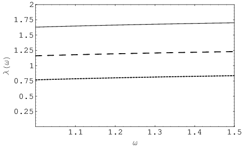
For Bs​0→Ds​(Ds∗)​l​ν¯B_{s0}\to D_{s}(D_{s}^{*})l\bar{\nu}, Θ⁡[Bs​0,Ds]\Theta[B_{s0},D_{s}] and Θ⁡[Bs​0,Ds∗]\Theta[B_{s0},D_{s}^{*}] can be obtained after replacing χ⁡(ω)\chi(\omega) by λ⁡(ω)\lambda(\omega) in Eq. (27)-(28), where

λ⁡(ω)=ZH​ZS​[ℬ1−ℬ2+ms]α=ΔS,β=ΔH.\displaystyle\lambda(\omega)=\sqrt{Z_{H}Z_{S}}[\mathcal{B}_{1}-\mathcal{B}_{2}+m_{s}]_{\alpha=\Delta_{S},\beta=\Delta_{H}}. (30)

Similarly, one gets the functions Θ⁡[Bs​1′,Ds]\Theta[B_{s1}^{\prime},D_{s}] and Θ⁡[Bs​1′,Ds∗]\Theta[B_{s1}^{\prime},D_{s}^{*}] for Bs​1′→Ds​(Ds∗)​ℓ​ν¯B_{s1}^{\prime}\to D_{s}(D_{s}^{*})\ell\bar{\nu} with the replacement ζ⁡(ω)→λ⁡(ω)\zeta(\omega)\to\lambda(\omega) in Eqs. (23)-(24).

IV Numerical results

We now collect the input parameters: GF=1.1664×10⁻⁵G_{F}=1.1664\times 10^{-5} GeV-2, Vc​b=0.043V_{cb}=0.043; MBs​1=5829.4M_{B_{s1}}=5829.4 MeV, MBs​2∗=5839.6M_{B_{s2}^{*}}=5839.6 MeV, MDs=1968.2M_{D_{s}}=1968.2 MeV, MDs∗=2112.0M_{D^{*}_{s}}=2112.0 MeV, MDs​J∗​(2317)=2317.3M_{D_{sJ}^{*}(2317)}=2317.3 MeV, MDs​J​(2460)=2458.9M_{D_{sJ}(2460)}=2458.9 MeV [3]. MBs​0=5718M_{B_{s0}}=5718 MeV and MBs​1′=5765M_{B_{s1}^{\prime}}=5765 [5]. ms=0.5m_{s}=0.5 GeV, Λ=1.25\Lambda=1.25 GeV, the infrared cutoff μ=0.593\mu=0.593 GeV and ΔS−ΔH=335±35\Delta_{S}-\Delta_{H}=335\pm 35 MeV [27].

In Table 6, we give the ranges of ΔH,S,T\Delta_{H,S,T} for the strange sector, which are given in Ref. [27, 28]. In terms of the definitions of ZH,S,TZ_{H,S,T} in Eqs. (9)-(11), we obtain the values of ZH,S,TZ_{H,S,T} listed in Table 6.

Type ΔH\Delta_{H} ΔS\Delta_{S} ΔT\Delta_{T} ZHZ_{H} ZSZ_{S} ZTZ_{T}
(a) 0.5 0.86 0.84 4.87 2.95 3.26
(b) 0.6 0.91 0.94 3.45 2.28 1.91
(c) 0.7 0.97 1.04 2.37 1.66 1.06
Table 6: The values of ΔH,S,T\Delta_{H,S,T} and the corresponding ZH,S,TZ_{H,S,T}. Here ΔH,S,T\Delta_{H,S,T} and ZH,S,TZ_{H,S,T} are in units of GeV and GeV-1, respectively.

With the above parameters, Fig. 2 illustrates the dependence of the form factors ξ⁡(ω)\xi(\omega), ζ⁡(ω)\zeta(\omega), χ⁡(ω)\chi(\omega) and λ⁡(ω)\lambda(\omega) on ω\omega.

Refer to caption
Refer to caption
(a) (b)
Refer to caption
Refer to caption
(c) (d)
Figure 2: (a) The dependence of ξ⁡(ω)\xi(\omega) on ω\omega. Here the solid, dashed and dotted lines correspond to the results with parameters (ΔT=0.84,ΔH=0.5)(\Delta_{T}=0.84,\Delta_{H}=0.5), (ΔT=0.94,ΔH=0.6)(\Delta_{T}=0.94,\Delta_{H}=0.6), (ΔT=1.04,ΔH=0.7)(\Delta_{T}=1.04,\Delta_{H}=0.7), respectively. (b) The variation of ζ⁡(ω)\zeta(\omega) with ω\omega. Here the solid, dashed and dotted lines correspond to the results with parameters (ΔT=0.84,ΔS=0.86)(\Delta_{T}=0.84,\Delta_{S}=0.86), (ΔT=0.94,ΔS=0.91)(\Delta_{T}=0.94,\Delta_{S}=0.91), (ΔT=1.04,ΔS=0.97)(\Delta_{T}=1.04,\Delta_{S}=0.97), respectively. (c) The dependence of χ⁡(ω)\chi(\omega) on ω\omega. Here the solid, dashed and dotted lines correspond to the results with parameters ΔS=0.86\Delta_{S}=0.86, ΔS=0.91\Delta_{S}=0.91, ΔS=0.97\Delta_{S}=0.97, respectively. (d) The variation of λ⁡(ω)\lambda(\omega) with ω\omega. Here the solid, dashing and dotted lines correspond to the results with parameters (ΔS=0.86,ΔH=0.5)(\Delta_{S}=0.86,\Delta_{H}=0.5), (ΔS=0.91,ΔH=0.6)(\Delta_{S}=0.91,\Delta_{H}=0.6), (ΔS=0.97,ΔH=0.7)(\Delta_{S}=0.97,\Delta_{H}=0.7), respectively.

In Tables 7 and 8, we give the decay widths of the semileptonic decays of Bs​1B_{s1}, Bs​2∗B_{s2}^{*}, Bs​0B_{s0} and Bs​1′B_{s1}^{\prime} with the three different choices of parameters ΔH,S,T\Delta_{H,S,T} listed in Table 6. Up to now, the CDF and D0 collaborations have not measured the decay widths of Bs​1B_{s1} and Bs​2∗B_{s2}^{*}.

Bs​1→B_{s1}\to Bs​2∗→B_{s2}^{*}\to
(a) (b) (c) (a) (b) (c)
Ds​ℓ​ν¯D_{s}\ell\bar{\nu} 2.1×10−152.1\times 10^{-15} 1.8×10−151.8\times 10^{-15} 1.6×10−151.6\times 10^{-15} 2.1×10−152.1\times 10^{-15} 1.8×10−151.8\times 10^{-15} 1.6×10−151.6\times 10^{-15}
Ds∗​ℓ​ν¯D_{s}^{*}\ell\bar{\nu} 4.9×10−154.9\times 10^{-15} 4.4×10−154.4\times 10^{-15} 3.9×10−153.9\times 10^{-15} 5.0×10−155.0\times 10^{-15} 4.5×10−154.5\times 10^{-15} 3.9×10−153.9\times 10^{-15}
Ds​0​ℓ​ν¯D_{s0}\ell\bar{\nu} 8.7×10−208.7\times 10^{-20} 4.7×10−204.7\times 10^{-20} 6.9×10−206.9\times 10^{-20} 5.6×10−205.6\times 10^{-20} 3.0×10−203.0\times 10^{-20} 4.5×10−204.5\times 10^{-20}
Ds​1′​ℓ​ν¯D_{s1}^{\prime}\ell\bar{\nu} 1.0×10−191.0\times 10^{-19} 8.7×10−208.7\times 10^{-20} 1.5×10−191.5\times 10^{-19} 1.2×10−191.2\times 10^{-19} 1.0×10−191.0\times 10^{-19} 1.8×10−191.8\times 10^{-19}
Table 7: The decay widths of the semileptonic decays of Bs​1B_{s1} and Bs​2∗B_{s2}^{*}. Here columns (a), (b), (c) correspond to the results with the three parameter combinations listed in Table 6. The decay widths are in units of GeV.
Bs​0→B_{s0}\to Bs​1′→B_{s1}^{{}^{\prime}}\to
(a) (b) (c) (a) (b) (c)
Ds​ℓ​ν¯D_{s}\ell\bar{\nu} 2.5×10−142.5\times 10^{-14} 1.3×10−141.3\times 10^{-14} 5.9×10−155.9\times 10^{-15} 1.2×10−141.2\times 10^{-14} 6.4×10−156.4\times 10^{-15} 2.9×10−152.9\times 10^{-15}
Ds∗​ℓ​ν¯D_{s}^{*}\ell\bar{\nu} 2.5×10−152.5\times 10^{-15} 1.3×10−141.3\times 10^{-14} 5.9×10−155.9\times 10^{-15} 3.8×10−143.8\times 10^{-14} 2.0×10−142.0\times 10^{-14} 9.1×10−159.1\times 10^{-15}
Ds​0​ℓ​ν¯D_{s0}\ell\bar{\nu} 1.6×10−151.6\times 10^{-15} 3.9×10−163.9\times 10^{-16} 2.8×10−152.8\times 10^{-15} 4.9×10−164.9\times 10^{-16} 9.6×10−169.6\times 10^{-16} 3.7×10−153.7\times 10^{-15}
Ds​1′​ℓ​ν¯D_{s1}^{\prime}\ell\bar{\nu} 1.5×10−151.5\times 10^{-15} 3.3×10−153.3\times 10^{-15} 1.3×10−141.3\times 10^{-14} 2.1×10−152.1\times 10^{-15} 2.7×10−152.7\times 10^{-15} 1.2×10−141.2\times 10^{-14}
Table 8: The decay widths of the semileptonic decays of Bs​0B_{s0} and Bs​1′B_{s1}^{\prime}. Here columns (a), (b), (c) correspond to the results with the three parameter combinations listed in Table 6. The decay widths are in units of GeV.
Refer to caption
Refer to caption
(a) (b)
Refer to caption
Refer to caption
(c) (d)
Figure 3: (a), (b), (c) and (d) illustrate the dependence of the differential rates of the semileptonic decays of Bs​1B_{s1} on ω\omega. Here the solid, dashed and dotted lines correspond to type (a), (b) and (c) in Table 6.

Using the semileptonic decays of Bs​1B_{s1} as an example, we show the variation of the differential rates of the semileptonic decays of Bs​1B_{s1} with ω\omega in Fig. 3. The differential rates of Bs​1→Ds​ℓ​ν¯B_{s1}\to D_{s}\ell\bar{\nu} and Bs​1→Ds∗​ℓ​ν¯B_{s1}\to D_{s}^{*}\ell\bar{\nu} increase with ω\omega monotonically. In contrast, the variation of the differential rates of Bs​1→Ds​0​ℓ​ν¯B_{s1}\to D_{s0}\ell\bar{\nu} and Bs​1→Ds​1′​ℓ​ν¯B_{s1}\to D_{s1}^{\prime}\ell\bar{\nu} with ω\omega are not monotonic. The different line shapes of the differential rates of the semileptonic decays of Bs​1B_{s1} account for the results of the decay widths in Table 7, i.e. it tells us why the decay rates for type (c) are not always larger than the results for the other types. The same observation holds for the semileptonic decays of Bs​2∗B_{s2}^{*}, Bs​0B_{s0}, Bs​1′B_{s1}^{\prime}.

V Discussion

The semileptonic decay of the bottom-strange meson is an interesting topic. Due to the lack of experimental information of the excited bottom-strange mesons, theorists mainly focused on the semileptonic decay of BsB_{s} using theoretical approaches such as the QCD sum rule approach [29] and the quark model [26]. The observations of Bs​1B_{s1} and Bs​2∗B_{s2}^{*} [1, 2] enrich the mass spectrum of the bottom-strange system greatly. In this work, in order to explore the possibility of searching the semileptonic decays of the excited bottom-strange states in the experiments, we have calculated Bs​0,Bs​1′,Bs​1,Bs​2∗→[Ds​(1968),Ds∗​(2112),Ds​J​(2317),Ds​J​(2460)]​ℓ​ν¯B_{s0},\,B_{s1}^{\prime},\,B_{s1},\,B_{s2}^{*}\to[D_{s}(1968),\,D_{s}^{*}(2112),\,D_{sJ}(2317),\,D_{sJ}(2460)]\ell\bar{\nu} in the framework of the CQM model.

Our numerical results indicate that (1) the decay width of Bs​1​(Bs​2∗)→Ds​(Ds∗)​ℓ​ν¯B_{s1}(B_{s2}^{*})\to D_{s}(D_{s}^{*})\ell\bar{\nu} is around 10−1510^{-15} GeV, which is 4∼54\sim 5 orders of magnitude larger than that of Bs​1​(Bs​2∗)→Ds​J​(2317,2460)​ℓ​ν¯B_{s1}(B_{s2}^{*})\to D_{sJ}(2317,2460)\ell\bar{\nu}; (2) the decay width of Bs​0​(Bs​1′)→Ds​(Ds∗,Ds​J​(2317,2460))​ℓ​ν¯B_{s0}(B_{s1}^{\prime})\to D_{s}(D_{s}^{*},D_{sJ}(2317,2460))\ell\bar{\nu} is 10−14∼10−1510^{-14}\sim 10^{-15} GeV.

Although the CDF and D0 experiments did not measure the decay widths of Bs​1B_{s1} and Bs​2∗B_{s2}^{*} and the experiments did not observe Bs​0B_{s0} and Bs​1′B_{s1}^{\prime}, we can roughly estimate the branching ratio of the semileptonic decay of Bs​1B_{s1}, Bs​2B_{s2}, Bs​0B_{s0} and Bs​1′B_{s1}^{\prime}. In Ref. [4], one obtains the two-body strong decay widths of Bs​1B_{s1} and Bs​2∗B_{s2}^{*} as 98 keV and 5 MeV respectively. Bs​0B_{s0} and Bs​1′B_{s1}^{\prime} are expected to be narrow resonances with a width around several tens of keV33 3 In Ref. [6], authors calculated the isospin-violating strong decay widths of Bs​0B_{s0} and Bs​1′B_{s1}^{\prime}, which are 35 keV and 38 keV, respectively. [6], since their main decay modes are the isospin violating strong decays and electromagnetic decays. Thus it is reasonable to take the strong decay width as the total width approximately for Bs​1B_{s1}, Bs​2B_{s2}, Bs​0B_{s0} and Bs​1′B_{s1}^{\prime}. We further show the order of magnitude of the semileptonic decay of Bs​1B_{s1}, Bs​2B_{s2}, Bs​0B_{s0} and Bs​1′B_{s1}^{\prime} in Table 9, which is convenient for the experimentalist to conclude whether the current and future experiments can reach these semileptonic decays.

Bs​0→B_{s0}\to Bs​1′→B_{s1}^{\prime}\to Bs​1→B_{s1}\to Bs​2∗→B_{s2}^{*}\to
Ds​ℓ​ν¯D_{s}\ell\bar{\nu} 10−9∼10−1010^{-9}\sim 10^{-10} 10−9∼10−1010^{-9}\sim 10^{-10} ∼10−11\sim 10^{-11} ∼10−13\sim 10^{-13}
Ds∗​ℓ​ν¯D_{s}^{*}\ell\bar{\nu} 10−9∼10−1010^{-9}\sim 10^{-10} 10−9∼10−1010^{-9}\sim 10^{-10} ∼10−11\sim 10^{-11} ∼10−13\sim 10^{-13}
Ds​0​ℓ​ν¯D_{s0}\ell\bar{\nu} 10−10∼10−1110^{-10}\sim 10^{-11} 10−10∼10−1110^{-10}\sim 10^{-11} ∼10−16\sim 10^{-16} ∼10−18\sim 10^{-18}
Ds​1′​ℓ​ν¯D_{s1}^{\prime}\ell\bar{\nu} 10−9∼10−1010^{-9}\sim 10^{-10} 10−9∼10−1010^{-9}\sim 10^{-10} ∼10−16\sim 10^{-16} ∼10−17\sim 10^{-17}
Table 9: The estimation of the branching fractions of the semileptonic decays of Bs​0B_{s0}, Bs​1′B_{s1}^{\prime}, Bs​1B_{s1} and Bs​2∗B_{s2}^{*} according to our numerical result shown in Table 7 and 8.

From Table 9, we can exclude the possibility of finding the semileptonic decay of Bs​2∗→[Ds,Ds∗,Ds​0,Ds​1′]​ℓ​ν¯B_{s2}^{*}\to[D_{s},\,D_{s}^{*},\,D_{s0},\,D_{s1}^{\prime}]\ell\bar{\nu} and Bs​1→[Ds​0,Ds​1′]​ℓ​ν¯B_{s1}\to[D_{s0},\,D_{s1}^{\prime}]\ell\bar{\nu} in experiments. However, for Bs​1→[Ds,Ds∗]​ℓ​ν¯B_{s1}\to[D_{s},\,D_{s}^{*}]\ell\bar{\nu} and the semileptonic decays of Bs​0B_{s0} and Bs​1′B_{s1}^{\prime}, the upper limit of the branching ratio can reach to 10−910^{-9}. The present precision of the experimental measurement of the branching fraction of the BB mesons has reached up to 10−7∼10−810^{-7}\sim 10^{-8} [3]. The decays Bs​1→[Ds,Ds∗]​ℓ​ν¯B_{s1}\to[D_{s},\,D_{s}^{*}]\ell\bar{\nu} and the semileptonic decays of Bs​0B_{s0} and Bs​1′B_{s1}^{\prime} may be observed in future experiments. Especially, the forthcoming LHCb experiments will produce an enormous amount of data of heavy-flavor hadrons, which is one of the potential experiments in which to search the Bs​1→[Ds,Ds∗]​ℓ​ν¯B_{s1}\to[D_{s},\,D_{s}^{*}]\ell\bar{\nu} and the semileptonic decays of Bs​0B_{s0} and Bs​1′B_{s1}^{\prime}. Then these semileptonic decays will be helpful to further test the structure of Ds​J​(2317)D_{sJ}(2317) and Ds​J​(2460)D_{sJ}(2460). In our calculation, we have assumed Ds​J​(2317)D_{sJ}(2317) and Ds​J​(2460)D_{sJ}(2460) as the charm-strange mesons with JP=0+J^{P}=0^{+} and 1+1^{+}. If the experimental measurement of these semileptonic decays are consistent with our prediction, it will provide strong support of the c​s¯c\bar{s} structure for Ds​J​(2317)D_{sJ}(2317) and Ds​J​(2460)D_{sJ}(2460).

Acknowledgments

This project was supported by the National Natural Science Foundation of China under Grants 10625521, 10721063, 10705001. X.L. was also supported by the Fundação para a Ciência e a Tecnologia of the Ministério da Ciência, Tecnologia e Ensino Superior of Portugal (SFRH/BPD/34819/2007).

Appendix

The definitions of ℐ0​(α)\mathcal{I}_{0}(\alpha), ℐ1\mathcal{I}_{1}, ℐ5​(α,β,ω)\mathcal{I}_{5}(\alpha,\beta,\omega), ℐ6​(α,β,ω)\mathcal{I}_{6}(\alpha,\beta,\omega), ℐ3​(α)\mathcal{I}_{3}(\alpha), 𝒜2​(α,β,ω)\mathcal{A}_{2}(\alpha,\beta,\omega), 𝒜3​(α,β,ω)\mathcal{A}_{3}(\alpha,\beta,\omega),ℬ1(α,β.ω)\mathcal{B}_{1}(\alpha,\beta.\omega) and ℬ2​(α,β,ω)\mathcal{B}_{2}(\alpha,\beta,\omega) are [20]

𝒜2​(α,β,ω)\displaystyle\mathcal{A}_{2}(\alpha,\beta,\omega)
=[(ω2−1)T(α,β,ω)−6ωU(α,β,ω)\displaystyle=[(\omega^{2}-1)T(\alpha,\beta,\omega)-6\omega U(\alpha,\beta,\omega)
+(2ω2+1)S(α,β,ω)+3S(β,α,ω)]/[2(ω2−1)2],\displaystyle\quad+(2\omega^{2}+1)S(\alpha,\beta,\omega)+3S(\beta,\alpha,\omega)]/[2(\omega^{2}-1)^{2}],
(31)
𝒜3​(α,β,ω)\displaystyle\mathcal{A}_{3}(\alpha,\beta,\omega)
=[−ω(ω2−1)T(α,β,ω)+2(2ω2+1)U(α,β,ω)\displaystyle=[-\omega(\omega^{2}-1)T(\alpha,\beta,\omega)+2(2\omega^{2}+1)U(\alpha,\beta,\omega)
−3ω(S(α,β,ω)+S(β,α,ω))]/[2(ω2−1)2]\displaystyle\quad-3\omega(S(\alpha,\beta,\omega)+S(\beta,\alpha,\omega))]/[2(\omega^{2}-1)^{2}] (32)
ℬ1​(α,β,ω)=[ω​X​(β,α,ω)−X⁡(α,β,ω)]/[ω2−1],\displaystyle\mathcal{B}_{1}(\alpha,\beta,\omega)=[\omega X(\beta,\alpha,\omega)-X(\alpha,\beta,\omega)]/[\omega^{2}-1], (33)
ℬ2​(α,β,ω)=[ω​X​(α,β,ω)−X⁡(β,α,ω)]/[ω2−1],\displaystyle\mathcal{B}_{2}(\alpha,\beta,\omega)=[\omega X(\alpha,\beta,\omega)-X(\beta,\alpha,\omega)]/[\omega^{2}-1], (34)

with

T⁡(α,β,ω)=ℐ6​(α,β,ω)+ms2​ℐ5​(α,β,ω),\displaystyle T(\alpha,\beta,\omega)=\mathcal{I}_{6}(\alpha,\beta,\omega)+m_{s}^{2}\mathcal{I}_{5}(\alpha,\beta,\omega), (35)
U⁡(α,β,ω)=ℐ1+α​ℐ3​(α)+β​ℐ3​(β)+α​β​ℐ5​(α,β,ω),\displaystyle U(\alpha,\beta,\omega)=\mathcal{I}_{1}+\alpha\mathcal{I}_{3}(\alpha)+\beta\mathcal{I}_{3}(\beta)+\alpha\beta\mathcal{I}_{5}(\alpha,\beta,\omega), (36)
S⁡(α,β,ω)=ω⁡[ℐ1+β​ℐ3​(β)]+α​ℐ3​(β)+α2​ℐ5​(α,β,ω),\displaystyle S(\alpha,\beta,\omega)=\omega[\mathcal{I}_{1}+\beta\mathcal{I}_{3}(\beta)]+\alpha\mathcal{I}_{3}(\beta)+\alpha^{2}\mathcal{I}_{5}(\alpha,\beta,\omega),
X⁡(α,β,ω)=−ℐ3​(β)−α​ℐ5​(α,β,ω),\displaystyle X(\alpha,\beta,\omega)=-\mathcal{I}_{3}(\beta)-\alpha\mathcal{I}_{5}(\alpha,\beta,\omega), (38)
ℐ0​(α)\displaystyle\mathcal{I}_{0}(\alpha) =\displaystyle= Nc16​π3/2​∫1/Λ21/μ2d​yy3/2​e−y⁡(ms2−α2)​(32​y+ms2−α2)\displaystyle\frac{N_{c}}{16\pi^{3/2}}\int_{1/\Lambda^{2}}^{1/\mu^{2}}\frac{dy}{y^{3/2}}e^{-y(m_{s}^{2}-\alpha^{2})}\left(\frac{3}{2y}+m_{s}^{2}-\alpha^{2}\right)
×[1+erf⁡(α​y)]−α​Nc​ms216​π2​Γ​(−1,ms2Λ2,ms2μ2),\displaystyle\times\left[1+\mathrm{erf}(\alpha\sqrt{y})\right]-\alpha\frac{N_{c}m_{s}^{2}}{16\pi^{2}}\Gamma\left(-1,\frac{m_{s}^{2}}{\Lambda^{2}},\frac{m_{s}^{2}}{\mu^{2}}\right),
ℐ1\displaystyle\mathcal{I}_{1} =\displaystyle= Nc​ms216​π2​Γ​(−1,ms2Λ2,ms2μ2),\displaystyle\frac{N_{c}m_{s}^{2}}{16\pi^{2}}\Gamma\left(-1,\frac{m_{s}^{2}}{\Lambda^{2}},\frac{m_{s}^{2}}{\mu^{2}}\right), (40)
ℐ3​(α)\displaystyle\mathcal{I}_{3}(\alpha) =\displaystyle= Nc16​π3/2​∫1/Λ21/μ2d​yy3/2​exp⁡[−y⁡(ms2−α2)]​(1+erf⁡(α​y)),\displaystyle\frac{N_{c}}{16\pi^{3/2}}\int^{1/\mu^{2}}_{1/\Lambda^{2}}\frac{dy}{y^{3/2}}\exp[-y(m_{s}^{2}-\alpha^{2})]\left(1+\mathrm{erf}(\alpha\sqrt{y})\right), (41)
ℐ5​(α,β,ω)\displaystyle\mathcal{I}_{5}(\alpha,\beta,\omega)
=∫01dx11+2​x2​(1−ω)+2​x​(ω−1)[2​Nc16​π3/2∫1/Λ21/μ2dyσe−y⁡(ms2−σ2)y−1/2(1+erf(σy))\displaystyle=\int_{0}^{1}dx\frac{1}{1+2x^{2}(1-\omega)+2x(\omega-1)}\Big[\frac{2N_{c}}{16\pi^{3/2}}\int_{1/\Lambda^{2}}^{1/\mu^{2}}dy\sigma e^{-y(m_{s}^{2}-\sigma^{2})}y^{-1/2}(1+\mathrm{erf}(\sigma\sqrt{y}))
+2​Nc16​π2∫1/Λ21/μ2dye−y​ms2y−1],\displaystyle+\frac{2N_{c}}{16\pi^{2}}\int_{1/\Lambda^{2}}^{1/\mu^{2}}dye^{-ym_{s}^{2}}y^{-1}\Big],
(42)
ℐ6​(α,β,ω)\displaystyle\mathcal{I}_{6}(\alpha,\beta,\omega)
=ℐ1​∫01d​x​σ1+2​x2​(1−ω)+2​x​(ω−1)−Nc16​π3/2​∫01d​x​11+2​x2​(1−ω)+2​x​(ω−1)\displaystyle=\mathcal{I}_{1}\int_{0}^{1}dx\frac{\sigma}{1+2x^{2}(1-\omega)+2x(\omega-1)}-\frac{N_{c}}{16\pi^{3/2}}\int_{0}^{1}dx\frac{1}{1+2x^{2}(1-\omega)+2x(\omega-1)}
×∫1/Λ21/μ2dyy−3/2e−y⁡(ms2−σ2){σ[1+erf(σy)][1+2y(ms2−σ2)]+2yπ[32​y+(ms2−σ2)]},\displaystyle\quad\times\int_{1/\Lambda^{2}}^{1/\mu^{2}}dyy^{-3/2}e^{-y(m_{s}^{2}-\sigma^{2})}\Big\{\sigma[1+\mathrm{erf}(\sigma\sqrt{y})][1+2y(m_{s}^{2}-\sigma^{2})]+2\sqrt{\frac{y}{\pi}}\left[\frac{3}{2y}+(m_{s}^{2}-\sigma^{2})\right]\Big\},

where

σ⁡(α,β,ω)=(1−x)​α+x​β1+2​x2​(1−ω)+2​x​(ω−1).\sigma(\alpha,\beta,\omega)=\frac{(1-x)\alpha+x\beta}{\sqrt{1+2x^{2}(1-\omega)+2x(\omega-1)}}.

References

  • [1] CDF Collaboration, T. Aaltonen et al., Phys. Rev. Lett. 100, 082001 (2008).
  • [2] D0 Collabotation, V.M. Abazov et al., arXiv:0711.0319 [hep-ex].
  • [3] W.M. Yao et al., Particle Data Group, J. Phys. G 33, 1 (2006).
  • [4] Z.G. Luo, X.L. Chen and X. Liu, arXiv:0901.0505 [hep-ph].
  • [5] W.A. Bardeen, E.J. Eichten and C.T. Hill, Phys. Rev. D 68, 054024 (2003); P. Colangelo, F. De Fazio and R. Ferrandes, Nucl. Phys. Proc. Suppl. 163, 177 (2007).
  • [6] J. Lu, W.Z. Deng, X.L. Chen, and S.-L. Zhu, Phys. Rev. D 73, 054012 (2006).
  • [7] The Babar Collaboration, B. Aubert et al., Phys. Rev. Lett. 90, 242001 (2003); F. Porter, Eur. Phys. J. C33, 219 (2004).
  • [8] The Belle Collaboration, P. Krokovny et al., Phys. Rev. Lett. 91, 262002 (2003).
  • [9] The CLEO Collaboration, D. Besson et al., Phys. Rev. D 68, 032002 (2003).
  • [10] S.L. Zhu, Int. J. Mod. Phys. E 17, 283-322 (2008).
  • [11] W.A. Bardeen, E.J. Eichten and C.T. Hill, Phys. Rev. D 68, 054024 (2003); M.A. Nowak, M. Rho and I. Zahed, Acta Phys. Polon. B 35, 2377 (2004); E. Kolomeitsev and M. Lutz, Phys. Lett. B 582, 39 (2004).
  • [12] K.T. Chao, Phys. Lett. B 599, 43 (2004).
  • [13] E. van Beveren and G. Rupp, Phys. Rev. Lett. 91, 012003 (2003); E. van Beveren and G. Rupp, Eur. Phys. J. C 32, 493 (2004).
  • [14] Y. B. Dai, C. S. Huang, C. Liu, S. L. Zhu, Phys. Rev. D 68, 114011 (2003).
  • [15] S. Narison, Phys. Lett. B 605, 319 (2005).
  • [16] Y. B. Dai, X. Q. Li, S. L. Zhu and Y. B. Zuo, Eur. Phys. J. C 55, 249 (2008), arXiv: hep-ph/0610327.
  • [17] Y.Q. Chen and X.Q. Li, Phys. Rev. Lett. 93, 232001 (2004); A.P. Szczepaniak, Phys. Lett. B 567, 23 (2003); T.E. Browder, S. Pakvasa and A.A. Petrov, Phys. Lett. B 578, 365 (2004).
  • [18] H.Y. Cheng and W.S. Hou, Phys. Lett. B 566, 193 (2003).
  • [19] T. Barnes, F.E. Close and H.J. Lipkin, Phys. Rev. D 68 054006 (2003); A.P. Szczepaniak, Phys. Lett. B 567, 23 (2003).
  • [20] A. Deandrea, N. Di Bartolomeo, R. Gatto, G. Nardulli and A. D. Polosa, Phys. Rev. D 58, 034004 (1998); A.D. Polosa, Riv. Nuovo Cim. 23N11, 1, 2000.
  • [21] D. Ebert, T. Feldmann and H. Reinhardt, Phys. Lett. B 388, 154 (1996); T. Feldmann, arXiv: hep-ph/9606451; D. Ebert, T. Feldmann, R. Friedrich and H. Reinhardt, Nucl. Phys. B 434 619 (1995).
  • [22] A.F. Falk and M.E. Luke, Phys. Lett. B 292, 119 (1992).
  • [23] A. Deandrea, N. Di Bartolomeo, R. Gatto, G. Nardulli and A.D. Polosa, Phys. Rev. D 58, 034004 (1998); A. Deandrea, R. Gatto, G. Nardulli and A.D. Polosa, Phys.Rev. D 59, 074012 (1999); A. Deandrea, R. Gatto, G. Nardulli and A.D. Polosa, J. High Energy Phys. 02, 021 (1999); A. Deandrea, R. Gatto, G. Nardulli and A.D. Polosa, Phys. Rev. D 61, 017502 (1999); A.D. Polosa, arXiv: hep-ex/9909371.
  • [24] X.H. Guo, H.W. Ke, X.Q. Li, X. Liu and S.M. Zhao, Commun. Theor. Phys. 48, 509-518 (2007), arXiv:hep-ph/0510146.
  • [25] X. Liu, Y.M. Yu, S.M. Zhao and X.Q. Li, Eur. Phys. J. C 47, 445 (2006), arXiv:hep-ph/0510146.
  • [26] S.M. Zhao, X. Liu and S.J. Li, Eur. Phy. J. C 51, 601-606 (2007), arXiv:hep-ph/0612008.
  • [27] A. Deandrea, G. Nardulli and A.D. Polosa, Phys. Rev. D 68, 097501 (2003).
  • [28] A.Deandrea, R.Gatto, G.Nardulli and A.D.Polosa, JHEP 9902 021 (1999).
  • [29] M.Q. Huang, Phys. Rev. D 69, 114015 (2004); T.M. Aliev and M. Savci, Phys. Rev. D 73 114010 (2006); T.M. Aliev, K. Azizi and A. Ozpineci, Eur. Phys. J. C 51, 593-599 (2007), arXiv: hep-ph/0608264.