Department of Physics \degreeDoctor of Philosophy in Physics \degreemonthApril \degreeyear2008 \thesisdateApril 24, 2008
Peter FisherProfessor of Physics
Thomas GreytakAssociate Department Head for Education
Model Independent Search For New Physics At The Tevatron
The Standard Model of elementary particles can not be the final theory. There are theoretical reasons to expect the appearance of new physics, possibly at the energy scale of few TeV. Several possible theories of new physics have been proposed, each with unknown probability to be confirmed. Instead of arbitrarily choosing to examine one of those theories, this thesis is about searching for any sign of new physics in a model-independent way. This search is performed at the Collider Detector at Fermilab (CDF).
The Standard Model prediction is implemented in all final states simultaneously, and an array of statistical probes is employed to search for significant discrepancies between data and prediction. The probes are sensitive to overall population discrepancies, shape disagreements in distributions of kinematic quantities of final particles, excesses of events of large total transverse momentum, and local excesses of data expected from resonances due to new massive particles.
The result of this search, first in 1 fb-1 and then in 2 fb-1, is null, namely no considerable evidence of new physics was found.
| Στους γονείς μου, Χρήςτο ϰαι Ευαγγελία, ςτην αδελφή μου Σοφία, ϰαι ςτον Επίϰουρο. | To my parents, Christos and Evangelia, my sister Sophia, and to Epicurus. |
Acknowledgments
I am indebted to my advisor, Bruce Knuteson. He has been extremely supportive, and mentored me optimally from the first day. I was given the opportunity to participate in many conferences, seminars and summer schools. He offered me space to develop initiative and apply my own ideas. For anyone who knows Bruce, he can only be a paradigm of perseverance and brightness.
It has been a big pleasure to work with Conor Henderson, our post-doc, on both hardware and analysis. Conor has been to me a resourceful teacher, and effective project leader. My classmate, Si Xie, who joined CDF later, has been a great person to work with, and I wish him the best as he may continue this project after I graduate. With Khaldoun Makhoul, Si, Conor, Bruce, and Markus Klute for a while, we advanced Level3 and Event Builder to their best. For this I also thank Ron Rechenmacher, who at times saved the day like deus ex machina.
Ray Culbertson contributed to this analysis both technically and mentally. His office has the heaviest traffic in CDF, to which I contributed with my visits for questions, so my thanks are due. The same for Stephen Mrenna, who has been very helpful as a theorist and event generator expert.
I thank for their support the CDF spokesmen, Rob Roser and Jaco Konigsberg; the Physics Coordinator, Doug Glenzinski; our godparents, Louis Lyons, Andy Hocker, Guillelmo Gomez-Ceballos, and Michael Schmidt who passed away prematurely; our reviewers, Al Goshaw, Sergey Klimenko and Mario Martinez-Perez; our conveners, Ben Brau and Chris Hays. They all worked very hard to bring this analysis to the community.
It is an honor to have my thesis evaluated by Physicists of the caliber of Jerry Friedman, Roman Jackiw and Peter Fisher.
I wish to thank many distinguished scientists at MIT for inviting me to their elite company. I may name indicatively Wit Busza, Bolek Wyslouch, Christoph Paus, Bernd Surrow, Gabriella Sciolla, and Richard Yamamoto. Finally, I warmly thank Steve Pavlon, the sweetest person I met in America.
Chapter 1 Introduction
1.1 The Standard Model
Our current understanding of nature on its most fundamental level is encoded in the “Standard Model” of elementary particles.
The building blocks of matter are categorized into three families of fermions and four gauge bosons, shown in Fig. 1.1.

The Standard Model is a local gauge invariant quantum field theory, which describes electromagnetic, weak and strong interactions. Interactions are introduced for free with the assumption that nature is symmetric under local gauge transformations of the group [1]. Electromagnetic and weak interactions are aspects of a unified electroweak interaction, which are distinguishable in result of electroweak symmetry breaking via the Higgs mechanism. Elementary particles acquire bare mass by coupling to the same Higgs field that is responsible for the electroweak symmetry breaking. The success of this model of electroweak interactions in describing experimental data from the last 35 years builds confidence in the existence of the Higgs boson, though it has not been directly observed as of today.
The Standard Model carries 26 free parameters, which are determined experimentally. Depending on how one counts, they are the 6 lepton masses, the 6 quark masses, 4 parameters from CKM plus 4 from PMNS matrix, the strong coupling , the QCD angle , the electromagnetic coupling , Weinberg angle , the vacuum expectation value () and the mass () of the Higgs.
The success of the Standard Model is certainly among the greatest achievements in physics. At the same time, it is bound to not be the final theory. Some reasons are explained in Section 1.1.1.
1.1.1 Limitations
The most obvious shortcoming of the Standard Model, as it stands, is that it does not describe gravity [2, 3]. Its domain is limited to energies much smaller than Planck mass (), where from dimensional analysis gravity is expected to be comparable to the other three known interactions.
Another nuisance is the presence of 26 free parameters. Past successful theories have established in our minds some notion of scientific aesthetics, according to which the fundamental theory should be able to derive, from first principles, numbers such as the mass of the electron, or the amount of CP violation observed in systems like and mesons. Otherwise one can not claim to understand those effects. Grand Unification Theories try to address these issues by embedding the Standard Model into larger symmetry groups (Sec. 1.2.1).
There is overwhelming evidence (from observations of the cosmic microwave background radiation, galaxy rotations, gravitational lensing, spectroscopy of clusters and super-novae) that dark matter and dark energy dominate the mass-energy density of the universe [4]. Currently, the Standard Model fails to provide a good candidate for either.
Another puzzle is the so-called “hierarchy problem”, namely why the electroweak symmetry is broken at energy 1 TeV, so much smaller than , where gravity becomes significant. Theories involving extra dimensions propose some answers (Sec. 1.2.3).
Related to hierarchy is the the problem of “naturalness” in the Standard Model. A small parameter in a theory is “natural” when setting it to zero increases some symmetry of the theory, therefore its smallness can be attributed to that very symmetry. For instance, the masslessness of a vector field such as the photon can be related to the gauge invariance of the theory. However, for a scalar field, such as the Standard Model Higgs, no symmetry is there to protect its mass from acquiring quadratically divergent corrections at the loop level (Fig. 1.3), unless the theory is highly fine-tuned (Fig. 1.2). The required precision of fine-tuning depends on how far one wishes to extend the validity of the Standard Model. If one wishes it account for loop corrections up to the Planck scale, while keeping the Higgs lighter than 1 TeV, as required by electroweak measurements, then the required fine-tuning is so precise that it seems unnatural (hence the connection between naturalness and hierarchy). A solution to this can be either to abandon the concept of fundamental scalars, as in technicolor models (Sec. 1.2.4), or to search for a theory where quadratic divergences cancel, as in Supersymmetry (Sec. 1.2.2).

 |
 |
| (a) | (b) |
1.2 Beyond the Standard Model
Let me summarize the main proposals which address the limitations explained in Sec. 1.1.1, and what observable implications each suggests.
1.2.1 Grand Unification
The motivation behind Grand Unification Theories (GUTs) [6, 7] are questions such as “why protons and electrons have exactly opposite charge”, or “why have three generations of fermions and three interactions”. These questions could become less thorny if instead of many we had just one symmetry group, which would make all particles look like components of just one particle, and all interactions like aspects of one force. Such a theory wouldn’t only satisfy common taste, but more importantly could derive from mathematical principles the values of some constants, such as , which would be a significant advancement in our understanding nature from a reductionist’s point of view.
Several Lie algebras have been studied; notably , , and more [2, 3]. Phenomenology varies significantly depending on the assummed symmetry. An effect predicted typically is proton decay, as new gauge bosons such as the one in Fig. 1.4, are predicted in breaking these hyper-symmetries at some large energy, typically GeV.
1.2.2 Supersymmetry
| Particle | Spin | Superpartner | Spin |
|---|---|---|---|
| Photon | 1 | Photino | 1/2 |
| Gluon | 1 | Gluino | 1/2 |
| 1 | Wino | 1/2 | |
| 1 | Zino | 1/2 | |
| 0 | Higgsino | 1/2 | |
| Graviton | 2 | Gravitino | 3/2 |
| Electron | 1/2 | Selectron | 0 |
| Muon | 1/2 | Smuon | 0 |
| Tau | 1/2 | Stau | 0 |
| Neutrino | 1/2 | Sneutrino | 0 |
| Quark | 1/2 | Squark | 0 |
Supersymmetric theories take the approach of solving the problem of naturalness (Sec. 1.1.1), by having a bosonic loop for each fermionic one, thus canceling out the quadratically divergent loop corrections.
SUSY introduces boson partners to Standard Model fermions, and fermion partners to gauge bosons. It introduces operators which transform fields into “superpartners” which differ from the original particles by half a unit of spin [8]. The superpartners of gauge bosons are called “gauginos”, those of leptons “sleptons” and those of quarks “squarks” (Table 1.1).
SUSY can have additional favorable features, which increase interest in it. With the extra assumption of a conserved multiplicative quantum number (R-parity), which is +1 for ordinary particles and -1 for superpartners, the lightest superpartner becomes stable, serving as a cold dark matter candidate [9]. Furthermore, a theory of local supersymmetry should lead to invariance under general coordinate transformations, which may be the road to incorporating General Relativity into the Standard Model. Finally, SUSY can affect the running of couplings to make them exactly equal at some energy, in compliance with Grand Unification Theories.
If supersymmetry were exact, then each Standard Model particle would have a superpartner of equal mass. Since this is not observed, SUSY has to be broken at some energy scale [3]. It is non-trivial to construct models where SUSY is broken in ways that avoid contradicting observation, and simultaneously do not destroy its desirable features.
Higgs mass is predicted to be of order GeV, so for SUSY to secure it from divergences it has to be introduced at energy 1 TeV. That happens to be also the energy scale where it needs to be introduced in order to equalize couplings at the scale of GeV, associated with Grand Unification. These elements hint that, if SUSY is a correct theory, it may be within reach for current experiments.
Most SUSY signatures involve large missing energy accompanied by multiple leptons and jets. Missing energy would be the effect of stable and elusive superpartners, while jets and leptons would result from long decay chains of unstable ones.
1.2.3 Extra Dimensions
Theories of extra dimensions are motivated by the hierarchy problem.
One hypothesis is that of large extra dimensions, where the known 4 dimensions, i.e. our “brane”, are embedded in a manifold of higher dimensionality, and gravity only appears to be feeble because part of it is projected onto our brane, while the rest propagates in the extra dimensions, often referred to as “the bulk”. By adjusting the number of extra dimensions and their radius of curvature, one can make gravity appear significant at and still lower its natural scale down to the electroweak scale [10].
Theories with universal extra dimensions exist too, where fermions and/or gauge bosons also propagate in the bulk [11].
Other theories assume wrapped extra dimensions. Hierarchy then emerges by exploiting the metric of the bulk space itself. For example, with one wrapped extra dimension periodically bounded by two 3-dimensional branes, Einstein’s equations result in an anti de Sitter metric, whose exponential factor makes gravity appear feeble on one of the 3-branes, where the Standard Model fields are supposed to be confined [12].
If at small distances gravity is not as feeble as suggested macroscopically by , then collider experiments could reveal the coupling of gravitons. For example, a signature could be , i.e. mono-jet events with large missing energy due to the graviton escaping in the bulk (Fig. 1.5). Another signature of the graviton could be the Standard-Model-forbidden [3]. In the case of universal extra dimensions one may observe the Kaluza-Klein higher states of fermions and bosons, through for instance.
1.2.4 Technicolor
An alternative approach to electroweak symmetry breaking, which avoids the introduction of fundamental scalar fields, is new strong dynamics. With the introduction of a new non-abelian gauge symmetry and additional fermions (“technifermions”) which have this new interaction, it becomes possible to form a technifermion condensate that can break the chiral symmetry of fermions, in a way analogous to QCD where the condensate breaks the approximate symmetry down to . The breaking of global chiral symmetries implies the existence of Goldstone bosons, the “technipions” (), in analogy with QCD pions. Three of the Goldstone bosons are absorbed through the Higgs mechanism to become the longitudinal components of the and , which then acquire mass proportional to the technipion decay constant.
Experimental signatures of technicolor are model dependent. For example, they can be the resonance of a Standard Model gauge boson into an excited technivector meson, like a technirho (), which subsequently decays into and , with possibly decaying to regular quarks [3]. For example, assuming that couples preferably to the third generation, such a process could be , or .
1.2.5 Compositeness
Compositeness is the idea that the Higgs and possibly other bosons and fermions contain substructure. Compositeness addresses the problem or naturalness similarly with technicolor, namely by avoiding the assumption of a fundamental scalar particle.
If quarks and leptons are not elementary, then they are predicted to have excited states (). For example, excited leptons could appear via or .
More importantly, if quarks and leptons have structure, new interactions should appear between them at the energy scale of their binding energy. They would be contact interactions, allowing processes such as and to occur in ways additional to those of the SM (Fig. 1.6) [13, 3].
| (a) | (b) |
1.3 Current standpoint - Motivation
In 1995, the discovery of the top quark was announced [14], leaving Higgs as the only unobserved Standard Model particle. We now enter the Large Hadron Collider (LHC) era with some confidence that the Higgs will be observed to complete the Standard Model pantheon of particles. At the same time, there is hope that even what has to lie beyond the Standard Model will be revealed soon. If such a groundbreaking discovery is made, it will be different from the top quark or even a possible Higgs discovery, in the sense that it will signify the opening to a new continent of unexplored physics.
Nature has proven its capacity to surprise us. There are many ideas of what the new physics may be, but there is no need for any of them to be right. So, especially in this historical time when we expect to overcome the current impasse, it makes sense to search for any sign of discrepancy between the data and the Standard Model, without introducing any bias in what it may look like. This is the motivation behind performing a model-independent and global search.
Tevatron stands at the current high energy frontier, producing collisions at energy 1.96 TeV and constantly increasing luminosity. Although the size and reach of the Tevatron are inferior to those of LHC, there is still a window of opportunity in the former, until the latter has collected data and understood systematic effects specific to it. It would be undesirable to discover something at the LHC and then look back only to realize that it had been overlooked at the Tevatron. On the other hand, performing a global, model-independent analysis of the Tevatron data has the potential of revealing evidence of new physics that can be cross-checked at the LHC. This hope motivates the present work.
Chapter 2 Experimental apparatus
The present search for new physics is performed in data collected with Collider Detector at Fermilab (CDF), a general scope detector for particles generated at high energy collisions produced by the Tevatron accelerator. Tevatron and the Fermi National Accelerator Laboratory (FNAL) are shown in Fig. 2.1.
This chapter describes the production of collisions and the CDF detector. For the many acronyms used, please consult Appendix D.

2.1 Beam Production
Either due to CP violation or some other unknown reason, free protons outnumber antiprotons, which makes it easier to obtain the former, and use them to generate the latter. In this section, the procedure leading to the production of the and beams is outlined.
2.1.1 Source
The production starts with storing hydrogen gas () in a Cockroft-Walton chamber [15], in which a 750 kV DC voltage causes electric discharges which produce negative hydrogen ions (). The are separated from the rest of the gas by use of a magnetic transport system and are channeled to the Linac.
The Linac [16] is a 130 m long Alvarez linear accelerator that transfers the from the Cockroft-Walton to the Booster, accelerating them from 750 keV to 400 MeV.
The Booster [17] is a 475 m long synchrotron that accelerates the from 400 MeV to 8 GeV in just 67 ms, hence its name. One Linac load is 40 s long and the rotation period of the beam in the Booster during injection is 2.22 s, which means that in principle it could take of the Linac’s load in 18 turns. Operationally however, only 5 or 6 turns get used for maximum intensity, and the rest (66.7%) of the Linac’s load is dumped. At the entrance, the ions pass through a carbon foil, which strips off the electrons, transforming into , viz. protons. It is important that the pass through the carbon foil at their entrance to the ring, as they meet with the circulating . This technique, named CEI, allows for higher beam brightness, avoiding limitations that would have otherwise followed from Liouville’s theorem [18]. A full Booster “batch” contains a maximum of protons at 8 GeV, coalesced into 84 bunches, ready to be delivered to the Main Injector.
2.1.2 Main Injector
The Main Injector [19] is a 3.319 km long non-circular synchrotron, serving not only the Tevatron, but also providing protons for the production of the NuMI neutrino beam and the proton beam in the Fixed Target area. Its operations that relate to the Tevatron are:
- 1.
production: A single Booster batch is injected into the MI at 8 GeV. These protons are accelerated to 120 GeV and extracted in a single turn for delivery to the production target. The produced antiprotons will eventually return to the MI for acceleration to 150 GeV, before they are delivered to the Tevatron.
- 2.
Collider mode: Accelerate protons or antiprotons to 150 GeV and deliver them to the Tevatron.
- 3.
End of store: Accept 150 GeV antiprotons and decelerate them to 8 GeV for storage in the Recycler.
2.1.3 Source
At the production area, the 120 GeV protons coming from the MI are directed onto a nickel target [20]. Before the collision, the bunch undergoes some modulation called RF bunch rotation, so as to be shorter in time and, in agreement with Liouville’s theorem, contain a wider spectrum of momenta. Its being more sudden maximizes the phase-space density of antiprotons produced as secondary products of the collision with the nickel target. First, the cone of particles produced at the collision is rendered parallel by means of a lithium lens [21]. Then, a dipole magnet selects 8 GeV antiprotons, as that is the standard MI injection energy, and directs them into the Debuncher.
At the Debuncher [20], which is a “ring” of rounded triangular shape, the 8 GeV antiprotons are subjected to a RF bunch rotation, this time in the reverse direction, so that their beam contains a narrower spectrum of momenta and, in agreement with Liouville’s theorem, spans a longer time interval. This reduction in momentum spread is done to improve the Debuncher-to-Accumulator transfer, because of the limited momentum aperture of the Accumulator at injection. The Debuncher makes use of the time between MI cycles to reduce the beam transverse size and longitudinal momentum spread through betatron and momentum stochastic cooling respectively. This further improves the efficiency of the Debuncher-to-Accumulator transfer.
The Accumulator [20] is a rounded triangular “ring”, similar to the Debuncher. The reason for that is that it also applies stochastic cooling to the beam, which requires linear segments along the ring to accommodate pickups and kickers. The main purpose of the Accumulator is to hold antiprotons until they are needed by the Tevatron. The antiprotons are stored in the Accumulator for hours or days, while they augment as more are produced at the nickel target. When a new pulse of antiprotons enters the Accumulator, it circulates along a trajectory of greater “radius” than the antiprotons that have already been cooled down. The RF decelerates the recently injected pulses of antiprotons from the injection energy to the edge of the stack tail. The stack tail momentum cooling system sweeps the beam deposited by the RF away from the edge of the tail and decelerates it towards the dense portion of the stack, known as the core. Additional cooling systems keep the antiprotons in the core at the desired momentum and minimize the transverse beam size.
There is yet another ring, the Recycler [22], which has a role similar to that of the Accumulator. It is a 3.3 km long ring along the MI, being therefore much longer than the Accumulator, which means that if the Accumulator is getting full it can use the Recycler to hold some antiprotons too. Spread over a longer ring, the antiprotons in the Recycler are easier to maintain stable, since the beam is less dense and the dispersive forces weaker. In addition to being longer, the Recycler employs the electron cooling method to reduce the momentum spread of the antiprotons. Electron cooling is a more modern technique than stochastic cooling, in which a cold (small momentum spread) beam of electrons travels parallel to the hot antiproton beam, serving as a heat sink, where the heat of the antiproton beam is dumped, since the two beams interact electromagnetically and from thermodynamics it is known that heat goes from the hotter system to the cooler. Once the electron beam heats up, it is discarded for a new, cold electron beam to take over. The Recycler does not only accept antiprotons that the Accumulator can not hold, but also those that the Tevatron does not need any more. Since antiprotons are so hard to produce, the Recycler keeps them to be reused in the next “store”, hence its name. When the stored antiprotons reach adequate quantity, the Tevatron is ready to start collisions.
2.1.4 Tevatron
For over two decades, the Tevatron [23, 3] has been the largest hadron collider, to be soon succeeded by the Large Hadron Collider (LHC) at CERN. It is a synchrotron accelerator with radius 1 km. Along its ring are 774 dipole and 216 quadrupole superconductive magnets, providing magnetic field of intensity 4.4 T. The magnets operate in superconductive state, with cooling from liquid helium.
The Tevatron receives and bunches from the MI, where they have been accelerated from 8 to 150 GeV. The filling takes about 30 minutes, much longer than the acceleration period that is only 86 seconds. It accelerates the and the beam to the energy of GeV, producing head-on collisions at TeV in the reference frame of CDF [3]. The proton and antiproton beams are both separated in 3 trains, each containing 12 bunches, therefore there are 36 and 36 bunches traveling in opposite directions at the same energy. Each bunch is about 18 ns (57 cm) long, which is the length of one RF bucket11 1 A RF bucket is a slot defined by the RF electromagnetic waves, in which a bunch may be accommodated. at the Tevatron. The interval between successive bunch crossings is 396 ns (21 buckets), which is of course equal to the interval between successive bunches in a train. Successive trains are separated by longer (2621 ns or 139 buckets) intervals, called abort gaps.
2.2 The CDF detector
CDF is a 5,000 ton detector [26] enveloping the B0 collision point of the Tevatron (Fit. 2.1). Externally, it looks forward-backward symmetric (Fig 2.2), mostly made of steel, of dimensions that are approximately . It is underground, shielded behind tons of concrete, which keeps it somewhat insulated from environmental sources of noise and prevents potentially hazardous radiation from leaking into its immediate surroundings. A three story building houses in its basement the detector and its assembly site, while in the superjacent levels it accommodates the data acquisition devices and the Control Room, from where operations are managed.


The CDF detector allows for a broad range of physics searches, from heavy flavor physics to searches of exotic new phenomena. It combines a variety of features, i.e. tracking, timing, calorimetry and muon detection systems, all seamed together with powerful trigger and DAQ systems.
By 1996, when the Run I period of Tevatron was over, about 90 of data had been collected, in which the long-sought -quark had eventually been discovered [14]. In preparation for the even more ambitious Run II era, which started in 2001, CDF was decisively upgraded [26], with new tracking and calorimetry capabilities and a much more efficient muon detection system. The DAQ system had to be upgraded too, to respond to the expected instantaneous luminosity of up to . In the following sections, the current status of CDF will be described.
2.2.1 Coordinate Systems
Before describing the most important CDF components, it would be useful to present the established system of coordinates used at the experiment.
The Cartesian coordinate system has its axes starting at the detector’s center, where the beams of and are supposed to collide. The axis is defined to point vertically up, and the to be perpendicular to the beam pipe and pointing in the direction away from the center of the Tevatron ring. In terms of and , is , which approximately coincides with the direction in which the beam travels through the center of CDF.
The cylindrical coordinate system reflects the approximate axial symmetry of the tracker and the calorimeter around , which in cylindrical coordinates remains the same unit vector it was in Cartesian. The radial unit vector at each point is perpendicular to and pointing away from the axis. The azimuthal angle is by definition on the semi-infinite plane that contains the positive axis and increases in the direction of .
Spherical coordinates are used more often than the above two systems. The reason is that, to the physical event occurring in a scattering, the cylindrical or any other symmetry of the surrounding detector is irrelevant. The dynamics of the event recognize one special axis, viz. , along which the and were traveling right before their collision. It is therefore convenient to define the angles of all outcoming particles with respect to . For any point in space, a radial unit vector is defined to point in the direction away from the beginning of the coordinates. Also, a polar angle is defined, which is along the positive axis and increases in the direction of . Finally, the azimuthal angle is defined as in the cylindrical coordinates and increases along .
Since the and beams are unpolarized, has to be an axis of symmetry when examining a large set of events. In other words, based on the premise of isotropy of the universe which leaves as the only axis special to the scattering, there can be no law of physics that would cause a non-uniform distribution of the particles coming out of the scattering.
It is common to not mention the polar angle per se, but instead a dimensionless quantity called “pseudorapidity”, which is related to as
| (2.1) |
is the limit of the quantity called ‘‘rapidity’’, which is22 2 The rapidity may not be confused with the Cartesian coordinate .
| (2.2) |
and has the beautiful property that for any pair of rapidities, the difference is invariant under Lorentz boosts along the axis.
2.2.2 Tracking
Tracking is crucial for particle identification; it has been so since the first experiments with wire and bubble chambers. Though technology has advanced, the principles remain:
- •
Only ionizing particles leave tracks, which distinguishes them from neutral ones.
- •
The curvature of a track under the influence of Lorentz force in the presence of a magnetic field is a measure of the transverse momentum of the particle, namely of the projection of its momentum on the plane transverse to .
- •
The direction of the track can be used to estimate the direction (,) in which a particle is produced.
- •
Being able to observe tracks improves our intuitive understanding of what particles are produced in an event. For example, the assembly of tracks within a cone is indicative of hadronic jet showers, while isolated tracks are more likely leptons33 3 Even though is a lepton, it is common to include only electrons and muons in the term “leptons”, because they are easier to identify than which often decays hadronically, so they consist more “clear” leptons in the experimental sense..
- •
Extrapolating the tracks of an event down to their origin(s) indicates the position of the event. This can reveal the existence of displaced secondary vertices, indicative of the decay of a long-lived particle, such as a meson. It may also indicate the existence of multiple interactions in the same bunch crossing, by observation of multiple primary vertices in the same event.
Silicon Detector
The first tracking device particles pass through is the Silicon Detector. Silicon allows for a highly granular and radiation tolerant tracker that can survive as near as 1.5 cm from the collision point [26]. The operation principle of a silicon micro-strip is depicted in Fig. 2.4 [3, 27].
About 722,000 read-out channels come from the Silicon Detector [28], by far more than from any other CDF component. It is separated in three subsystems: L00, SVX and ISL (Fig. 2.5, 2.6).
L00 is a single layer of single-sided silicon built directly onto the beam pipe, at 1.5 cm radius. It provides precision position measurement before the particles undergo multiple scattering.
SVX is the heart of the Silicon Detector, consisting of 12 identical wedges in . Each wedge contains 5 layers of double-sided silicon, oriented parallel to the beam pipe at radii from 2.5 to 10.6 cm. On one side, the silicon strips are aligned axially. The other side has stereo strips for 3 of the layers, and stereo strips for the remaining 2 layers. Obviously, the choice of aligning some strips non-axially was made to allow for three-dimensional track reconstruction.
The ISL envelops SVX. It carries stereo double-sided silicon in a single layer for intermediate radius measurement of central44 4 Here and below the word “central” is used to describe objects with ; “plug” is used to describe objects with . tracks and in two layers for tracking in the region , which is not completely covered by the COT (Fig. 2.6).
The silicon embedded strips are 8 m wide [29], which brings the hit’s spatial resolution down to about 12 m. This resolution makes it possible to measure the impact parameter of a track to 40 m, with 30 m uncertainty due to the beam width. The , namely the -coordinate of the primary vertex, can be measured with 70 m accuracy.


Central Outer Tracker
The COT [30, 31] is a cylindrical multi-wire open-cell drift chamber surrounding the Silicon Detector (Fig. 2.6).
COT contains Argon-Ethane () in a 1:1 mixture. When charged particles traverse the gaseous mixture they leave a trail of ionization electrons, which drift under the influence of an 1.9 kV/cm electric field. The latter is produced by field planes and homogenized by potential and shaper wires. After some time that depends on the distance they travel, the ionization electrons are collected by sense wires immersed in the gas producing a detectable55 5 When an ionization electron approaches the 40m thick sense wire it is accelerated by its rapidly increasing () electric field, producing an “avalanche” of secondary ionization electrons and thus enhancing the signal. electric signal. The location of the track with respect to the sense wire is then estimated from the time it takes to detect the signal. The drift distance is less than 0.88 cm and is covered in less than 100 ns, which is less than the 396 ns between successive bunch crossings, therefore causes no pile-up of signals from different events.
The field panels, shape, potential and sense wires are all grouped in electrostatically shielded cells (Fig. 2.7). Each cell contains 12 sense, 13 potential and 4 shaper wires. Sense and potential wires alternate with successive sense wires being 7mm apart. Combining drift time information from several wires, the single hit resolution reduces to about 140 m.

Cells are arranged in 8 superlayers (Fig. 2.8). The wires in the and superlayer are not oriented axially, but at a stereo angle of . Similarly, there is a stereo angle of in superlayers 3 and 7. Like in the case of the Silicon Detector, the reason that 4 out of the 8 superlayers are oriented non-axially is to allow for tracking in the three dimensions66 6 If all COT wires were parallel to the axis, then the coordinate of hits would be unknown..

It was mentioned that ionization electrons drift under the influence of an electric field , but there is also a magnetic field parallel to the axis. So, as the force accelerates the electron, the force turns it on the plane (Fig. 2.9). At any time the velocity of the electron in the medium can be parametrized as , where is the mobility of the medium. Assuming that the field is homogeneous on the plane and the electron is non-relativistic, the equilibrium is at an angle with respect to that is . is called the Lorentz angle and for the COT it is about . The wires in the COT cells are then arranged along the direction determined by the Lorentz angle, to minimize the drift time and maximize the COT efficiency and resolution (Fig. 2.7).

Magnet
A 1.4 T magnetic field is produced in the direction by the superconductive solenoid surrounding the COT (Fig. 2.6 and 2.3).
The magnetic field is essential for the measurement of the transverse momentum () of ionizing particles. Greater magnetic field intensity and bigger tracking volume radius improve resolution, which on the other hand is limited by the spatial resolution of the tracker and multiple scattering [3]. At CDF, the resolution is .
Track reconstruction
The Silicon Detector and the COT record a large number of hits in each event, viz. discrete positions from which ionizing particles seem to have passed. But the hits alone do not suffice. In each event there are tens of charged particles, as well as false hits. What is needed is an algorithm to reconstruct tracks out of the thousands of hits of each event.
Every track is a helix that can be parametrized in terms of the variables in Table 2.1. Essentially, tracking algorithms fit for those 5 parameters to best match the observed hits [32, 33].
| the polar angle at minimum approach, which refers to the point of the track closest to the axis. | |
| semi-curvature of the track (inverse of diameter), with the same sign as the particle’s electric charge. | |
| coordinate at minimum approach. | |
| signed impact parameter: distance between helix and the axis at minimum approach. The sign of is given from its formal definition: , where is the ionizing particle’s charge, (,) is the center of the track’s projection onto the plane, and is the radius of the same projection. Fig. 2.10 demonstrates combinations of positive and negative and . | |
| Direction of track on plane at minimum approach, i.e. the polar angle of the particle’s at minimum approach. |

Tracking in the COT using the Segment Linking algorithm involves first reconstructing linear segments of the track in each of the eight superlayers [33]. Then, the linear segments from the axial layers are linked to form a 2D track on the plane, starting the extrapolation with the outmost segment as seed. The projection of the track is attained by linking the segments from the stereo superlayers. Eventually, the track is characterized by the of the fit, and is only kept if that figure of merit is below threshold.
An alternative is the Histogram Tracking algorithm [33]. It starts with a coarse approximation of the final track, which is attained by extrapolating a segment of the track called “telescope”, such as the outer superlayer segment. The extrapolated telescope corresponds to a helix whose parameters carry large uncertainty, therefore instead of a curve it can imagined as a tube, to visualize those uncertainties (Fig. 2.11). In each layer the tube crosses there may be hits that fall inside the tube. For those hits, the likelihood is calculated to belong to the track. Each crossed layer is translated into a histogram of those likelihoods. Those histograms coming from different layers are then combined into a final one, and the track is reconstructed as the helix which maximizes the combined likelihood. Compared to the Segment Linking algorithm, this alternative is slower but more efficient in cases of missing and accurate in cases of spurious hits.

The Histogram Tracking algorithm is also applied in Silicon tracking, where the part of the track in the COT is used as the telescope.
In Silicon tracking [33], the information of the of the primary vertex is used. That is known by combining hits from the stereo strips and extrapolating to the beam axis. This produces a variety of candidates, each of different likelihood, so in the end the primary vertex is at the most likely .
The Stand-Alone algorithm for Silicon tracking uses information exclusively from silicon hits, therefore has the advantage of using the whole acceptance of the Silicon Detector. It starts by finding hits in places where axial and stereo strips intersect. Then, triplets of aligned hits are identified. The information of the primary vertex is used to constrain the candidate helices. In the end the best fitting helix is kept.
The Outside-In algorithm [34] takes COT tracks and extrapolates them into the Silicon Detector, adding hits via a progressive fit. As each layer of silicon is encountered, a road size is established based on the error matrix of the track. Hits that are within the road are added to the track, and the track parameters and error matrix are refit with this new information. A new track candidate is generated for each hit in the road, and each of these new candidates are then extrapolated to the next layer in, where the process is repeated. As the extrapolation proceeds, the track error matrix is inflated to reflect the amount of scattering material encountered. At the end of this process, there may be many track candidates associated with the original COT track. The candidate that has hits in the largest number of silicon layers is chosen as the winner; if more than one candidate has the same number of hits, the of the fit in the silicon is used to decide.
The Inside-Out algorithm [35] performs the reverse extrapolation: from the Silicon Detector to the COT. Its goal is to use the Stand-Alone silicon track to associate it with COT hits and improve the efficiency of reconstruction of tracks that do not cross more than 4 COT superlayers.
2.2.3 Calorimetry
CDF is equipped with sampling electromagnetic and hadronic calorimeters in the central and plug region, enhanced with shower maximum and preshower detectors for improved particle identification [26]. Central calorimeters cover rads in (Fig. 2.2). The central electromagnetic calorimeter covers and the hadronic . The plug calorimeters reach as far as . They are segmented in wedge-shaped towers pointing to the center of CDF. Each tower covers about 0.1 units of and in (Fig. 2.3). For increased acceptance, the hadronic calorimeter has the endwall calorimeter, spanning (Fig. 2.6).
Electromagnetic Calorimeter
CEM and PEM comprise lead absorber sheets alternating with scintillator layers. Light produced at the scintillator is transfered by WLS fibers to two PMTs that correspond to each tower77 7 Having two PMTs per tower allows for cross-check of the validity of signals, using time information and comparing the difference in the signal intensity in the two..
The CEM has a total maximum thickness of about 19 , in 20-30 (varying with ) layers of 3 mm lead and 5 mm scintillator. Its energy resolution, after in situ calibration, is found to be .
PEM contains 22 layers of lead, 4.5 mm each88 8 The first layer is an exception, being 1 cm thick and read out separately to be used as a preshower detector., and its scintillator layers are 4 mm thick. Its total thickness is 21 . Its resolution is .
In both CEM and PEM, there is a shower maximum detector, 6 into the calorimeter, where an electromagnetic shower statistically contains the biggest number of particles [3]. CES is a multi-wire proportional chamber with strip readout in the direction and wire along . PES has scintillator strips that cross to form a 2-dimensional grid in each plug. With resolution of about 2 mm in the central and 1 mm in the plug, the showermax detectors facilitate the matching of tracks with calorimeter hits, improving identification. Also, sampling the profile of the electromagnetic showers at 6 allows for improved identification.
Finally, between the solenoid and the first layer of the CEM lies a set of multi-wire proportional chambers, the CPR, which samples the electromagnetic showers at 1.075 , viz. the solenoid’s thickness. This information greatly enhances and soft identification [26].
Hadronic Calorimeter
The hadronic calorimeter is similar to the electromagnetic, except that it uses iron for absorber instead of lead. The CHA is 4.7 thick, consisting of 32 2.5 cm iron layers alternating with 1 cm scintillator layers. Its energy resolution is .
The WHA has similar energy resolution [36]; . It contains 15 layers of iron, 5 cm each, alternating with 1 cm layers of scintillator, adding up to 4.5 .
The PHA is thicker, containing 7 in 23 layers of iron, 51 mm each, alternating with 6 mm layers of scintillator. Its energy resolution is .
2.2.4 Muon System
CDF is equipped with four muon detectors (Fig. 2.12), which will be described in this section.
Muons weigh 200 times more than electrons, therefore radiate about times less by bremsstrahlung. They do not deposit much energy in the calorimeter, but rather traverse the whole detector almost unimpeded. This makes them easier to identify by installing wire chambers around the detector, beyond the calorimeter and even beyond extra absorbing material; muons are virtually the only ionizing particles that can reach there.
Shielding the muon detectors behind absorber increases the detected muons’ purity, but also enhances multiple scattering, which makes it harder to match the small track segment in the muon detector (called “stub”) with the corresponding COT track. However this is not a very big problem, especially for high- muons, since the displacement due to multiple scattering is about , for the is in GeV/c [26]. Furthermore, some low- muons can not reach the muon detectors, but that is not a problem either, since the threshold is lower than 2.2 GeV/c [26], far lower than the of the muons considered in this analysis.

Central Muon detector (CMU)
The CMU [26] surrounds the hadronic calorimeter, at radius 3.47 m, covering the region. It consists of argon-ethane wire chamber cells operating in proportional mode, organized in stacks of four. Each wire chamber is with a resistive stainless steel wire along its biggest dimension, which is aligned parallel to the axis. In it is segmented in 24 wedges, each containing 4 stacks side by side, therefore each wedge contains a chamber of cells (Fig. 2.13).

The drift times ( ns) are used to measure the projection of the track. The coordinate of the track is extracted with about 10 cm precision, using the charge division method, whose principle is explained in Fig. 2.14. To apply this method, every couple of adjacent cells have their wires ganged together at one end.

Central Muon Upgrade detector (CMP)
The CMP (Fig. 2.12) is shielded behind about 7.8 , comprising the calorimeter, the magnet return yoke and extra steel absorber. Compared to the CMU, which was shielded behind only 5 hadronic interaction lengths, the CMP provides higher purity in muon identification [26]. Those reconstructed muons that have a stub in both the CMU and the CMP are called “CMUP muons”.
The CMP is not azimuthally symmetric, but resembles a box surrounding the central region of the detector (). It is made of wire chambers similar to those used for the CMU, but just bigger: .
A bigger difference is that CMP contains scintillator counters in addition to wire chambers. The scintillator layers lie on the outer side of the chambers and provide timing information that is used to discard out-of-time muon candidates, which could not possibly be muons originating from the center of the detector. Furthermore, timing helps not have stubs from different bunch crossings piled up, given that the drift time in the CMP can be as large as 1.7 s [26]. Eventually, the dimensions of the scintillator counters are , so two silicon counters are needed to cover the dimension of the CMU, providing the very crude information of whether a muon stub has positive or the negative coordinate.
CMX
CMX [26] is very similar to CMP; it consists of same type wire chambers and silicon counters. It differs significantly in geometry though. It covers the region and is shaped like a conic section on each side of the detector (Fig. 2.12). The wire chambers are grouped in wedges, each in . Each wedge contains 48 chambers, arranged in 8 layers. The lower of the CMX, which physically penetrate the floor supporting the detector, are called “miniskirt” for obvious reason (Fig. 2.12). This part was not instrumented until past 2003.
IMU
2.2.5 Cerenkov Luminosity Counter
CDF is equipped with the CLC [37], a detector dedicated to measuring instantaneous luminosity (). It consists of Cerenkov counters placed in the far forward and backward region (). filled with isobutane at nearly atmospheric pressure.
The number of interactions () in a bunch crossing follows the Poisson distribution with mean , where is the cross section of inelastic scattering and is the time interval between bunch crossings.
Bunch crossings with occur with probability . By measuring the fraction of empty crossings can be measured99 9 Of course it is necessary to correct the measured by dividing with the CLC acceptance . and therefore .
An alternative method consists in measuring directly as , where is the number of CLC counts of some bunch crossing, and is the average number of CLC counts in the case of single-interaction bunch crossings. can be measured at low , when .
The first method, of measuring empty crossings, has the advantage of not needing any information such as , but at high empty crossings become rare, making this method inefficient. On the other hand, the second method depends on the information, and in reality does not scale linearly with , as the CLC occupancy grows and is eventually saturated due to the finite number of counters, therefore correction for this non-linearity are required.
The uncertainty in the integrated luminosity measured with the CLC is 6%, to which the biggest contribution comes from the uncertainty in at 1.96 TeV.
2.2.6 Data Acquisition
CDF employs approximately readout channels. A bunch crossing at yields on average about 5 interactions. An event of such multiplicity takes about 200 kB of digitized information volume. It becomes then obvious that not every single bunch crossing can be read, as that would require the enormous bandwidth of 630 GB/s.
Apart from technically inevitable, it is also sensible to record only those events that pass some quality selection and would be of some interest1010 10 In an experiment of the broad scope of CDF it is not trivial to decide which events could be of some interest, since different analyses may see interest in different kinds of events. Furthermore, nobody is certain what the signature of physics beyond the Standard Model will be.. For example, an event with leptons should be retained, while for multi-jet events it is enough to keep only a fraction of them, since they are so abundant in collisions.
The DAQ system [26] is responsible for selecting the best events as they occur. Fig. 2.15 provides an overview of the DAQ architecture.

Level-1
The frequency of 2.5 MHz at which bunches cross is too high to allow for full reconstruction of every event, so the first level of selection is based on fragments of information. This happens in Level-1; an accept/reject decision is made using “primitives”, namely coarse information on COT tracks and stubs in the CMU, CMP and CMX [26]. Systems providing primitives are depicted in Fig. 2.16. The XFT crudely reconstructs COT tracks on the plane. The XTRP extrapolates XFT tracks through the calorimeter and the muon system finding matching hits/towers.
Based on the primitives, several algorithms also called “individual triggers” contribute to the Level-1 decision. For example, effort is made to keep events with high- tracks, or leptons, or large missing transverse energy () etc.
The latency of Level-1 is 5.5 s, in which 14 bunch crossings occur. Therefore, all front-end electronics are equipped with buffers of enough capacity to contain information from 14 bunch crossings. Level-1 then works as a synchronous pipeline; by the time 14 events are pushed back into the buffer, at least one event has been examined and pulled from it, freeing a slot for the current event to be buffered.
Less than 2% of the events pass Level-1, making its accept rate less than 50 kHz.
Level-2
Level-2 functions as an asynchronous pipeline, where events are processed in FIFO mode [26]. With no more than kHz input rate, it can afford up to 1/50 kHz = 20 s to decide on each event1111 11 Actually, since up to 4 events can be kept in the Level-2 buffer, the latency can be even greater, without causing dead-time, provided that this is not the case for too many events..
In its decision, Level-2 takes into account the primitives of Level-1, in addition to showermax information, as shown in Fig. 2.16.

The acceptance rate of Level-2 is less than 1 kHz. Effort is made to maintain this rate as close to 1 kHz as possible, by readjusting the trigger requirements as changes, making them stricter at high and looser at low .
Event Builder
In the case of a Level-2 accept, the whole detector is eventually read out. The EVB collects the fragments of the event and passes them to Level-3. Reading out the front-end electronics of the whole detector takes about 1 ms, which is why this step is only possible after having discarded over 99.96% of the events.
EVB (Fig. 2.17) lies in 21 VME crates, each containing one Linux computer, referred to as SCPU [38]. Each crate is dedicated to reading a different part of the detector. Apart from the SCPU, each crate contains a series of memory buffers, the VRBs. When the front-end crates are read, the information of the event is first stored in the VRBs. Each SCPU reads the VRBs of it own crate through the VME backplane of the crate, which in combination with the GigaBit Ethernet networking allows for the desired system speed. On reading the VRBs, a byte-count check is performed, as well as checks of the size of each buffer entry [39]. Though in principle EVB should not be discarding any events, it does so if information is missing or corrupted.
The function of the EVB is coordinated by the EVB Proxy, a process running on a dedicated Linux machine. All acknowledgement messages within the EVB are circulated through the EVB Proxy, and so does any information exchanged with the TSI and Level-3.

Level-3
Level-3 is the last stage of trigger selection [38]. Receiving events from the EVB at kHz, it is purely software implemented, performing three basic functions:
- 1.
Concatenates same-event fragments coming from the EVB into an event entry.
- 2.
Imposes the final selection, taking into account the reconstructed objects information.
- 3.
Submits passing events to the CSL for storage.
There is a whole cluster of 411 Linux computers counting 2.4 THz of CPU dedicated to Level-3. Though all computers are nearly identical, they are separated in three categories, depending on their task:
- •
18 Converter nodes: They receive event fragments from the EVB and combine them to form self-contained event records which they pass to available Processor nodes.
- •
384 Processor nodes: Upon reception of events from a Converter, they apply the Level-3 filter to either discard or pass them to an Output node, after some reformatting that reshapes the passing entries to their final format.
- •
9 Output nodes: They receive the passing events from Processor nodes and propagate them to the CSL for storage.
The Level-3 cluster is separated in 18 identical subsets, called ‘‘subfarms’’1212 12 A term appropriate for a subdivision of the whole Level-3 cluster, which is called “farm” in CDF jargon.. This way, data handling proceeds in 18 independent, parallel streams which share the load of incoming events. Each subfarm contains 1 Converter, 21 or 22 Processors, and shares an Output with another subfarm. On every Processor, 5 Level-3 filters run simultaneously, on hyper-threaded dual-core Intel CPUs. The Converter of each subfarm is allowed to only submit events to Processors of its own subfarm, and the Processors of each subfarm can only send events to the Output node serving it.
The operation of Level-3 is coordinated by the Level-3 Proxy application, running on a dedicated computer. The Proxy collects and sends acknowledgements from and to the computers of the cluster, and communicates with the EVB Proxy to indicate among other things which Converter is available to receive the next event.
Filtering is done by a program written in C++, the Level-3 filter executable, which applies criteria stored in a centralized database implemented in Oracle. In the database is stored the trigger table, which is a list of “triggers”. Each trigger is structured to contain the following information:
- 1.
The prerequisite Level-1 and Level-2 triggers.
- 2.
The C++ reconstruction modules that should be used and in what order.
- 3.
The specific selection criteria decided having some physics goal, for example a cut in some invariant mass in the event.
- 4.
The name of the dataset in which to store the event if it passes the trigger selection.
The output rate of Level-3 is about 100 Hz. The events passing Level-3 are sent to the CSL for immediate storage. From there, they are shortly sent to the FCC for permanent storage on magnetic tape.
2.2.7 Off-line production
Data analysis is not performed on the raw data. Before the data on tape are usable, the off-line production process has to take place.
At production [26], the raw data banks are unpacked and physics objects are reconstructed in full detail. This is similar to what is done at Level-3, but the off-line reconstruction is much more elaborate, applying the latest calibrations, since those reconstructed objects will be the final ones to be used for analysis.
Since passing Level-3, each event contains the information of the dataset(s) it belongs to. At the production, even further partitioning is made; datasets are collections of filesets, which are collections of files containing events.
For the needs of each analysis, the raw data are taken from the appropriate dataset and are converted to a convenient format. Since ROOT [40] is the adopted analysis framework, the format varies between different architectures of ROOT Trees. For example, one is the “topNtuple”, used mostly by collaborators doing -quark analyses, but a more common format, used also in the present analysis, is the “Standard Ntuple” (Stntuple).
Chapter 3 Data Analysis
The analysis going into this thesis was conducted in two rounds: first with 1 fb-1 of data, and then with 2 fb-1. The first round has been documented in [41, 42, 43, 44]. An updated publication is currently being prepared for the second one. This chapter is an adaptation of [41], while chapter 4 presents material that will be in the publication of the second round.
3.1 Strategy
Sec. 1.3 motivates the goal of this analysis, viz. the model-independent search for new physics. The method is to obtain a satisfactory description of the Standard Model expectation in channels where high- data are observed, and employ an array of probes to seek for statistically significant discrepancies between data and Standard Model background.
Crucial for model-independence is to not focus on channels sensitive to particular models, but examine data in as many channels as possible. That introduces to this analysis over two million events (in 1 fb-1), ranging from abundant QCD to rare electroweak ones. Studying this large volume of qualitatively diverse data requires reducing the information content of each event to bare bones and characterizing each event in terms of physics objects that maintain the same meaning universally in any kind of event. In each event, the 4-momenta of any reconstructed physics objects in its final state are recorded. These objects can be leptons, photons, hadronic jets or missing energy.
Another ingredient of model-independence is to not segregate the data into “control” and “signal” regions a priori, namely into regions where new physics is assumed to not exist or to exist respectively. In most analyses control regions are predefined, to adjust correction factors, under the assumption that there is no new physics in those regions and that the extrapolation of correction factors from the control to the signal region is valid. However, what is considered control region in one analysis is often signal region in some other, so, to be as generic as possible, one needs to treat all data as signal and control regions simultaneously, to address the question “how well does the Standard Model implementation describe the data?” If there is indeed detectable new physics, then it will be impossible to achieve good agreement between data and Standard Model simultaneously in all regions. More in Sec. C.
The Standard Model prediction is implemented in three steps:
- 1.
Monte Carlo generation and matching [45] of samples simulating the Standard Model processes.
- 2.
CDF detector simulation, which models the detector response to the MC generated events. For that, the Geant-based package CDFsim is used.
- 3.
Fine-tuning of the outcome of CDFsim to account for theoretical and experimental correction factors.
Structurally, the analysis contains four parts:
- 1.
The Vista global fit, which adjusts and applies the correction model, providing the Standard Model background of the best possible global agreement with the data, exploiting the flexibility granted by the correction model.
- 2.
The Vista comparison, which examines the statistical significance of features in the bulk of all distributions and sorts the information in a comprehensive way.
- 3.
The Sleuth search, which focuses on the high- tails searching for excesses of data.
- 4.
The Bump Hunter search (present only for the second round of the analysis), which scans all mass variables for local excesses of data, potentially indicating a new resonance.
The above statistical probes are employed simultaneously, rather than sequentially. So, an effect highlighted by Sleuth prompts additional investigation of the discrepancy, usually resulting in a specific hypothesis explaining the discrepancy in terms of a detector effect or adjustment to the Standard Model prediction that is then fed back and tested for global consistency.
Statistical significance is a necessary but insufficient condition for discovery. A statistically significant discrepancy could be attributed to inaccuracy in the Standard Model implementation, or in modeling the detector response. These possibilities would need to be considered on a case-by-case basis. In the event of a significant discrepancy, the breadth of view of this analysis can be exploited to evaluate the plausibility of it being a detector effect or a problem in the Standard Model implementation.
Forming hypotheses for the cause of specific discrepancies, implementing those hypotheses to assess their wider consequences, and testing global agreement after the implementation are emphasized as the crucial activities for the investigator throughout the process of data analysis. This process is constrained by the requirement that all adjustments be physically motivated. The investigation and resolution of discrepancies highlighted by the algorithms is the defining characteristic of this global analysis 11 1 It is not possible to systematically simulate the process of constructing, implementing, and testing hypotheses motivated by particular discrepancies, since this process is carried out by individuals. The statistical interpretation of this analysis is made bearing this process in mind..
This search for new physics terminates when either a compelling case for new physics is made, or there remain no statistically significant discrepancies on which a new physics case can be made. In the former case, to quantitatively assess the significance of the potential discovery, a full treatment of systematic uncertainties must be implemented. In the latter case, it is sufficient to demonstrate that all observed effects are not in significant disagreement with an appropriate global Standard Model description.
3.2 Vista
This section describes Vista: object identification, event selection, estimation of Standard Model backgrounds, simulation of the CDF detector response, development of a correction model, and results.
3.2.1 Object identification
Energetic and isolated electrons, muons, taus, photons, jets, and -tagged jets with and GeV are identified according to CDF standard criteria. The same criteria are used for all events. The isolation criteria employed vary according to object, but roughly require less than 2 GeV of extra energy flow within a cone of in – space around each object.
Standard CDF criteria [46] are used to identify electrons () in the central and plug regions of the CDF detector. Electrons are characterized by a narrow shower in the central or plug electromagnetic calorimeter and a matching isolated track in the central gas tracking chamber or a matching plug track in the silicon detector.
Standard CDF muons () are identified using three separate subdetectors in the regions , , and [46]. Muons are characterized by a track in the central tracking chamber matched to a track segment in the central muon detectors, with energy consistent with minimum ionizing deposition in the electromagnetic and hadronic calorimeters along the muon trajectory.
Narrow central jets with a single charged track are identified as tau leptons () that have decayed hadronically [47]. Taus are distinguished from electrons by requiring a substantial fraction of their energy to be deposited in the hadron calorimeter; taus are distinguished from muons by requiring no track segment in the muon detector coinciding with the extrapolated track of the tau. Track and calorimeter isolation requirements are imposed.
Standard CDF criteria requiring the presence of a narrow electromagnetic cluster with no associated tracks are used to identify photons () in the central and plug regions of the CDF detector [48].
Jets () are reconstructed using the JetClu [49] clustering algorithm with a cone of size , unless the event contains one or more jets with GeV and no leptons or photons, in which case cones of are used. Jet energies are appropriately corrected to the parton level [50]. Since uncertainties in the Standard Model prediction grow with increasing jet multiplicity, up to the four largest jets are used to characterize the event; any reconstructed jets with -ordered ranking of five or greater are neglected and their energy is treated as unclustered, except in final states with small summed scalar transverse momentum containing only jets.
A secondary vertex -tagging algorithm is used to identify jets likely resulting from the fragmentation of a bottom quark () produced in the hard scattering [51].
Momentum visible in the detector but not clustered into an electron, muon, tau, photon, jet, or -tagged jet is referred to as unclustered momentum (uncl).
Missing momentum () is calculated as the negative vector sum of the 4-vectors of all identified objects and unclustered momentum. An event is said to contain a object if the transverse momentum of this object exceeds 17 GeV, and if additional quality criteria discriminating against fake missing momentum due to jet mismeasurement are satisfied 22 2 An additional quality criterion is applied to the significance of the missing transverse momentum in an event, requiring that the energies of hadronic objects can not be adjusted within resolution to reduce the missing transverse momentum to less than 10 GeV. The transverse components of all hadronic energy clusters in the event are projected onto the unit missing transverse momentum vector , and a “conservative” missing transverse momentum is defined, where the sum is over hadronic energy clusters in the event, and the hadronic energy resolution of the CDF detector has been approximated as , expressed in GeV. An event is said to contain missing transverse momentum if GeV and GeV..
3.2.2 Event selection
Events containing an energetic and isolated electron, muon, tau, photon, or jet are selected. A set of three level online triggers requires:
- •
a central electron candidate with GeV passing level 3, with an associated track having GeV and an electromagnetic energy cluster with GeV at levels 1 and 2; or
- •
a central muon candidate with GeV passing level 3, with an associated track having GeV and muon chamber track segments at levels 1 and 2; or
- •
a central or plug photon candidate with GeV passing level 3, with hadronic to electromagnetic energy less than 1:8 and with energy surrounding the photon to the photon’s energy less than 1:7 at levels 1 and 2; or
- •
a central or plug jet with GeV passing level 3, with 15 GeV of transverse momentum required at levels 1 and 2, with corresponding prescales of 50 and 25, respectively; or
- •
a central or plug jet with GeV passing level 3, with energy clusters of 20 GeV and 90 GeV required at levels 1 and 2; or
- •
a central electron candidate with GeV and a central muon candidate with GeV passing level 3, with a muon segment, electromagnetic cluster, and two tracks with GeV required at levels 1 and 2; or
- •
a central electron or muon candidate with GeV and a plug electron candidate with GeV, requiring a central muon segment and track or central electromagnetic energy cluster and track at levels 1 and 2, together with an isolated plug electromagnetic energy cluster; or
- •
two central or plug electromagnetic clusters with GeV passing level 3, with hadronic to electromagnetic energy less than 1:8 at levels 1 and 2; or
- •
two central tau candidates with GeV passing level 3, each with an associated track having GeV and a calorimeter cluster with GeV at levels 1 and 2.
Events satisfying one or more of these online triggers are recorded for further study. Offline event selection for this analysis uses a variety of further filters. Single object requirements keep events containing:
- •
a central electron with GeV, or
- •
a plug electron with GeV, or
- •
a central muon with GeV, or
- •
a central photon with GeV, or
- •
a central jet or -tagged jet with GeV, or
- •
a central jet or -tagged jet with GeV (prescaled by a factor of roughly ),
possibly with other objects present. Multiple object criteria select events containing:
- •
two electromagnetic objects (electron or photon) with and GeV, or
- •
two taus with and GeV, or
- •
a central electron or muon with GeV and a central or plug electron, central muon, or central tau with GeV, or
- •
a central photon with GeV and a central electron or muon with GeV, or
- •
a central or plug photon with GeV and a central tau with GeV, or
- •
a central photon with GeV and a central -jet with GeV, or
- •
a central jet or -tagged jet with GeV and a central tau with GeV (prescaled by a factor of roughly ), or
- •
a central or plug photon with GeV and two central taus with GeV, or
- •
a central or plug photon with GeV and two central -tagged jets with GeV, or
- •
a central or plug photon with GeV, a central tau with GeV, and a central -tagged jet with GeV,
possibly with other objects present. Explicit online triggers feeding this offline selection are required. The thresholds for these criteria are chosen to be sufficiently above the online trigger turn-on curves that trigger efficiencies can be treated as roughly independent of object .
Good run criteria are imposed, requiring the operation of all major subdetectors. To reduce contributions from cosmic rays and events from beam halo, standard CDF cosmic ray and beam halo filters are applied [52].
These selections result in a sample of roughly two million high- data events in an integrated luminosity of 927 pb-1.
3.2.3 Event generation
Standard Model backgrounds are estimated by generating a large sample of Monte Carlo events, using the Pythia [53], MadEvent [54], and Herwig [55] generators. MadEvent performs a leading order matrix element calculation, and provides 4-vector information corresponding to the outgoing legs of the underlying Feynman diagrams, together with color flow information. Pythia 6.218 is used to handle showering and fragmentation. The CTEQ5L [56] parton distribution functions are used.
QCD jets.
QCD dijet and multijet production are estimated using Pythia. Samples are generated with Tune A [57] with lower cuts on , the transverse momentum of the scattered partons in the center of momentum frame of the incoming partons, of 0, 10, 18, 40, 60, 90, 120, 150, 200, 300, and 400 GeV. These samples are combined to provide a complete estimation of QCD jet production, using the sample with greatest statistics in each range of .
.
The estimation of QCD single prompt photon production comes from Pythia. Five samples are generated with Tune A corresponding to lower cuts on of 8, 12, 22, 45, and 80 GeV. These samples are combined to provide a complete estimation of single prompt photon production in association with one or more jets, placing cuts on to avoid double counting.
.
QCD diphoton production is estimated using Pythia.
.
The estimation of +jets processes (with denoting or ), where the or decays to first or second generation leptons, comes from MadEvent, with Pythia employed for showering. Tune AW [57] is used within Pythia for these samples. The CKKW matching prescription [45] with a matching scale of 15 GeV is used to combine these samples and avoid double counting. Additional statistics are generated on the high- tails using the MLM matching prescription [58]. The factorization scale is set to the vector boson mass; the renormalization scale for each vertex is set to the of the jet. +4 jets are generated inclusively in the number of jets; +3 jets are generated inclusively in the number of jets.
.
The estimation of , , and production with zero or more jets comes from Pythia.
.
The estimation of and production comes from MadEvent, with showering provided by Pythia. These samples are inclusive in the number of jets.
.
Estimation of with zero or more jets comes from Pythia.
.
Estimation of with zero or more jets comes from Pythia.
.
Top quark pair production is estimated using Herwig assuming a top quark mass of 175 GeV and NNLO cross section of pb [59].
Remaining processes, including for example and , are generated by systematically looping over possible final state partons, using MadGraph [60] to determine all relevant diagrams, and using MadEvent to perform a Monte Carlo integration over the final state phase space and to generate events. The MLM matching prescription is employed to combine samples with different numbers of final state jets.
A higher statistics estimate of the high- tails is obtained by computing the thresholds in corresponding to the top 10% and 1% of each process, where denotes the scalar summed transverse momentum of all identified objects in an event. Roughly ten times as many events are generated for the top 10%, and roughly one hundred times as many events are generated for the top 1%.
Cosmic rays.
Backgrounds from cosmic ray or beam halo muons that interact with the hadronic or electromagnetic calorimeters, producing objects that look like a photon or jet, are estimated using a sample of data events containing fewer than three reconstructed tracks. This procedure is described in more detail in Appendix A.2.1.
Minimum bias.
Minimum bias events are overlaid according to run-dependent instantaneous luminosity in some of the Monte Carlo samples, including those used for inclusive and production. In all samples not containing overlaid minimum bias events, including those used to estimate QCD dijet production, additional unclustered momentum is added to events to mimic the effect of the majority of multiple interactions, in which a soft dijet event accompanies the rare hard scattering of interest. A random number is drawn from a Gaussian centered at 0 with width 1.5 GeV for each of the and components of the added unclustered momentum. Backgrounds due to two rare hard scatterings occurring in the same bunch crossing are estimated by forming overlaps of events, as described in Appendix A.2.2.
Each generated Standard Model event is assigned a weight, calculated as the cross section for the process (in units of picobarns) divided by the number of events generated for that process, representing the number of such events expected in a data sample corresponding to an integrated luminosity of 1 pb-1. When multiplied by the integrated luminosity of the data sample used in this analysis, the weight gives the predicted number of such events in this analysis.
3.2.4 Detector simulation
The response of the CDF detector is simulated using a geant-based detector simulation (CDFsim) [61], with gflash [62] used to simulate shower development in the calorimeter.
In collisions there is an ordering of frequency with which objects of different types are produced: many more jets () are produced than -jets () or photons (), and many more of these are produced than charged leptons (, , ). The CDF detectors and reconstruction algorithms have been designed so that the probability of misreconstructing a frequently produced object as an infrequently produced object is small. The fraction of central jets that CDFsim misreconstructs as photons, electrons, and muons is , , and , respectively. Due to these small numbers, the use of CDFsim to model these fake processes would require generating samples with prohibitively large statistics. Instead, the modeling of a frequently produced object faking a less frequently produced object (specifically: faking , , , , or ; or or faking , , or ) is obtained by the application of a misidentification probability, a particular type of correction factor in the Vista correction model, described in the next section.
In Monte Carlo samples passed through CDFsim, reconstructed leptons and photons are required to match to a corresponding generator level object. This procedure removes reconstructed leptons or photons that arise from a misreconstructed quark or gluon jet.
3.2.5 Correction model
| Code | Category | Explanation | Value | Error | Error(%) |
|---|---|---|---|---|---|
| 0001 | luminosity | CDF integrated luminosity | 927 | 20 | 2.2 |
| 0002 | -factor | cosmic | 0.69 | 0.05 | 7.3 |
| 0003 | -factor | cosmic | 0.446 | 0.014 | 3.1 |
| 0004 | -factor | 11 photon+jet(s) | 0.95 | 0.04 | 4.2 |
| 0005 | -factor | 12 | 1.2 | 0.05 | 4.1 |
| 0006 | -factor | 13 | 1.48 | 0.07 | 4.7 |
| 0007 | -factor | 14+ | 1.97 | 0.16 | 8.1 |
| 0008 | -factor | 20 diphoton(+jets) | 1.81 | 0.08 | 4.4 |
| 0009 | -factor | 21 | 3.42 | 0.24 | 7.0 |
| 0010 | -factor | 22+ | 1.3 | 0.16 | 12.3 |
| 0011 | -factor | 0 (+jets) | 1.453 | 0.027 | 1.9 |
| 0012 | -factor | 1 | 1.06 | 0.03 | 2.8 |
| 0013 | -factor | 2 | 1.02 | 0.03 | 2.9 |
| 0014 | -factor | 3+ | 0.76 | 0.05 | 6.6 |
| 0015 | -factor | 0 (+jets) | 1.419 | 0.024 | 1.7 |
| 0016 | -factor | 1 | 1.18 | 0.04 | 3.4 |
| 0017 | -factor | 2+ | 1.03 | 0.05 | 4.8 |
| 0018 | -factor | 2 | 0.96 | 0.022 | 2.3 |
| 0019 | -factor | 2 | 1.256 | 0.028 | 2.2 |
| 0020 | -factor | 3 | 0.921 | 0.021 | 2.3 |
| 0021 | -factor | 3 | 1.36 | 0.03 | 2.4 |
| 0022 | -factor | 4 | 0.989 | 0.025 | 2.5 |
| 0023 | -factor | 4 | 1.7 | 0.04 | 2.3 |
| 0024 | -factor | 5+ | 1.25 | 0.05 | 4.0 |
| 0025 | ID eff | central | 0.986 | 0.006 | 0.6 |
| 0026 | ID eff | plug | 0.933 | 0.009 | 1.0 |
| 0027 | ID eff | 0.845 | 0.008 | 0.9 | |
| 0028 | ID eff | 0.915 | 0.011 | 1.2 | |
| 0029 | ID eff | central | 0.974 | 0.018 | 1.8 |
| 0030 | ID eff | plug | 0.913 | 0.018 | 2.0 |
| 0031 | ID eff | central | 1 | 0.04 | 4.0 |
| 0032 | fake rate | plug | 0.045 | 0.012 | 27.0 |
| 0033 | fake rate | central | 9.71 | 1.9 | 2.0 |
| 0034 | fake rate | plug | 0.000876 | 1.8 | 2.1 |
| 0035 | fake rate | 1.157 | 2.7 | 2.3 | |
| 0036 | fake rate | 0.01684 | 0.00027 | 1.6 | |
| 0037 | fake rate | 0.00341 | 0.00012 | 3.5 | |
| 0038 | fake rate | 0.00038 | 4 | 10.5 | |
| 0039 | fake rate | central | 0.000265 | 1.5 | 5.7 |
| 0040 | fake rate | plug | 0.00159 | 0.00013 | 8.2 |
| 0041 | trigger | central, | 0.976 | 0.007 | 0.7 |
| 0042 | trigger | plug, | 0.835 | 0.015 | 1.8 |
| 0043 | trigger | , | 0.917 | 0.007 | 0.8 |
| 0044 | trigger | , | 0.96 | 0.01 | 1.0 |
Unfortunately some numbers that can not be determined from first principles enter the comparison between data and the Standard Model prediction. These numbers are referred to as “correction factors”. This correction model is applied to generated Monte Carlo events to obtain the Standard Model prediction across all final states.
Correction factors must be obtained from the data themselves. These factors may be thought of as Bayesian nuisance parameters. The actual values of the correction factors are not directly of interest. Of interest is the comparison of data to Standard Model prediction, with correction factors adjusted to whatever they need to be, consistent with external constraints, to bring the Standard Model into closest agreement with the data.
The traditional prescription for determining these correction factors is to “measure” them in a “control region” in which no signal is expected. This procedure encounters difficulty when the entire high- data sample is considered to be a signal region. The approach adopted instead is to ask whether a consistent set of correction factors can be chosen so that the Standard Model prediction is in agreement with the CDF high- data.
The correction model is obtained by an iterative procedure informed by observed inadequacies in modeling. The process of correction model improvement, motivated by observed discrepancies, may allow a real signal to be artificially suppressed. If adjusting correction factor values within allowed bounds removes a signal, then the case for the signal disappears, since it can be explained in terms of known physics. This is true in any analysis. The stronger the constraints on the correction model, the more difficult it is to artificially suppress a real signal. By requiring a consistent interpretation of hundreds of final states, Vista is less likely to mistakenly explain away new physics than analyses of more limited scope.
The 44 correction factors currently included in the correction model are shown in Table 4.2. These factors can be classified into two categories: theoretical and experimental. A more detailed description of each individual correction factor is provided in Appendix A.4.
Theoretical correction factors reflect the practical difficulty of calculating accurately within the framework of the Standard Model. These factors take the form of -factors, so-called “knowledge factors,” representing the ratio of the unavailable all order cross section to the calculable leading order cross section. Twenty-three -factors are used for Standard Model processes including QCD multijet production, W+jets, Z+jets, and (di)photon+jets production.
Experimental correction factors include the integrated luminosity of the data, efficiencies associated with triggering on electrons and muons, efficiencies associated with the correct identification of physics objects, and fake rates associated with the mistaken identification of physics objects. Obtaining an adequate description of object misidentification has required an understanding of the underlying physical mechanisms by which objects are misreconstructed, as described in Appendix A.1.
In the interest of simplicity, correction factors representing -factors, efficiencies, and fake rates are generally taken to be constants, independent of kinematic quantities such as object , with only five exceptions. The dependence of three fake rates is too large to be treated as approximately constant: the jet faking electron rate in the plug region of the CDF detector; the jet faking -tagged jet rate , which increases steadily with increasing ; and the jet faking tau rate , which decreases steadily with increasing . Two other fake rates possess geometrical features in – due to the construction of the CDF detector: the jet faking electron rate in the central region, because of the fiducial tower geometry of the electromagnetic calorimeter; and the jet faking muon rate , due to the non-trivial fiducial geometry of the muon chambers. After determining appropriate functional forms, a single overall multiplicative correction factor, determined by the global fit, is used
Correction factor values are obtained from a global fit to the data. The procedure is outlined here, with further details relegated to Appendix A.3.
Events are first partitioned into final states according to the number and types of objects present. Each final state is then subdivided into bins according to each object’s detector pseudorapidity () and transverse momentum (), as described in Appendix A.3.1.
Generated Monte Carlo events, adjusted by the correction model, provide the Standard Model prediction for each bin. The Standard Model prediction in each bin is therefore a function of the correction factor values. A figure of merit is defined to quantify global agreement between the data and the Standard Model prediction, and correction factor values are chosen to maximize this agreement, consistent with external experimental constraints.
Letting represent a vector of correction factors, for the bin
| (3.1) |
where is the number of data events observed in the bin, is the number of events predicted by the Standard Model in the bin, is the Monte Carlo statistical uncertainty on the Standard Model prediction in the bin 33 3 Given a set of Monte Carlo events with individual weights , so that the total Standard Model prediction from these Monte Carlo events is events, the “effective weight” of these events can be taken to be the weighted average of the weights: . The “effective number of Monte Carlo events” is , and the error on the Standard Model prediction is ., and is the statistical uncertainty on the expected data in the bin. The Standard Model prediction in the bin is a function of .
Relevant information external to the Vista high- data sample provides additional constraints in this global fit. The CDF luminosity counters measure the integrated luminosity of the sample described in this article to be 902 pb by measuring the fraction of bunch crossings in which zero inelastic collisions occur [63]. The integrated luminosity of the sample measured by the luminosity counters enters in the form of a Gaussian constraint on the luminosity correction factor. Higher order theoretical calculations exist for some Standard Model processes, providing constraints on corresponding -factors, and some CDF experimental correction factors are also constrained from external information. In total, 26 of the 44 correction factors are constrained. The specific constraints employed are provided in Appendix A.3.2.
The overall function to be minimized takes the form
| (3.2) |
where the sum in the first term is over bins in the CDF high- data sample with defined in Eq. 3.1, and the second term is the contribution from explicit constraints.
Minimization of in Eq. 3.2 as a function of the vector of correction factors results in a set of correction factor values providing the best global agreement between the data and the Standard Model prediction. The best fit correction factor values are shown in Table 4.2, together with absolute and fractional uncertainties. The determined uncertainties are not used explicitly in the subsequent analysis, but rather provide information used implicitly to assist in appropriate adjustment to the correction model in light of observed discrepancies. The uncertainties are verified by subdividing the data into thirds, performing separate fits on each third, and noting that the correction factor values obtained with each subset are consistent within quoted uncertainties. Further details on the correlation matrix and other technical aspects of this global fit can be found in Appendix A.3.3.
Although the correction factors are determined from a global fit, in practice the determination of many correction factors’ values are dominated by one recognizable subsample. The rate for a jet to fake an electron is determined largely by the number of events in the final state, since the largest contribution to this final state is from dijet events with one jet misreconstructed as an electron. Similarly, the rates and for a jet to fake a -tagged jet and tau lepton are determined largely by the number of events in the and final states, respectively. The determination of the fake rate , photon efficiency , and -factors for prompt photon production and prompt diphoton production are dominated by the , , and final states. Additional knowledge incorporated in the determination of fake rates is described in Appendix A.1.
The global fit per number of bins is 288.1 / 133 + 27.9, where the last term is the contribution to the from the imposed constraints. A per degree of freedom larger than unity is expected, since the limited set of correction factors in this correction model is not expected to provide a complete description of all features of the data. Emphasis is placed on individual outlying discrepancies that may motivate a new physics claim, rather than overall goodness of fit.
Corrections to object identification efficiencies are typically less than 10%; fake rates are consistent with an understanding of the underlying physical mechanisms responsible; -factors range from slightly less than unity to greater than two for some processes with multiple jets. All values obtained are physically reasonable. Further analysis is provided in Appendix A.4.
Final State Data Background 3j 5j 2j 2j bj 3j, high 3j b2j 3j, low 3j b5j j j b, low j j 2j, high b3j 8j 7j 6j 4j, low 4j, high 4j 4j 4j, low 4j 4j 4j 4j 4j 3j, low 3j 3j, high 3j 3j 3j 3j 3j 3j 3bj, low 2j, low 2j 2j 2j, low 2j, high 2j 2j 2j 2j 2j 2j 2j Final State Data Background 2j j 2b, low 2b, high 2b3j, high 2b2j, low 2b2j, high 2b2j 2b 2bj, low 2bj, high 2bj, low 2bj 2b2j 2b2j 2bj 2b j j j j, low j j j j j j j j j j 4j 4j 3j 3j 2j 2j 2j 2j 2j Final State Data Background j j j j j j j j 4j 3j 2j 2j j j j b6j b4j, low b4j, high b3j, low b3j, high b3j, low b3j b3j b3j b b2j, low b2j, high b2j, low b2j b2j b2j b b b b b bj, low bj, high bj bj bj, low bj bj bj bj b3j b2j b bj bj
 |
 |

With the details of the correction model in place, the complete Standard Model prediction can be obtained. For each Monte Carlo event after detector simulation, the event weight is multiplied by the value of the luminosity correction factor and the -factor for the relevant Standard Model process. The single Monte Carlo event can be misreconstructed in a number of ways, producing a set of Monte Carlo events derived from the original, with weights multiplied by the probability of each misreconstruction. The weight of each resulting event is multiplied by the probability the event satisfies trigger criteria. The resulting Standard Model prediction, corrected as just described, is referred to as “the Standard Model prediction” throughout the rest of this document, with “corrected” implied in all cases.
3.2.6 Results
Data and Standard Model events are partitioned into exclusive final states, depending on the combinations of reconstructed final objects. This partitioning is orthogonal, with each event ending up in one and only one final state, as shown schematically in Fig. 3.3. Data are compared to Standard Model prediction in each final state, considering the total number of events observed and predicted, and the shapes of relevant kinematic distributions.

In a data driven search, it is crucial to explicitly account for the trials factor, quantifying the number of places where we checked for an interesting signal. Purely statistical fluctuations at the level of three or more standard deviations are expected to appear, simply because a large number of regions are considered. A reasonably rigorous accounting of this trials factor is possible as long as the measures of interest and the regions to which these measures are applied are specified a priori, as is done here. In this analysis a discrepancy at the level of or greater after accounting for the trials factor (typically corresponding to a discrepancy at the level of or greater before accounting for the trials factor) is considered “significant.” It is worth noting that dedicated searches, checking only a small number of signal regions, typically do not account for any trials factor, simply because it is very difficult to quantify the effect of many people looking for new physics in different ways within the same experiment. For that reason, instead of a mild , a strong significance is considered necessary to discover something new in our field. The assumption made silently is that if one observes a effect in just one attempt, then if one could include somehow the trials factor, the actual significance of the observation would turn out to be still greater than , therefore convincing. However, in cases where the “new physics” is well-expected (like or dibosons, which are processes within the Standard Model) “discovery” is claimed even with just without considering the trials factor. Certainly, for physics beyond the Standard Model, a sans trials factor should not be considered convincing proof of existence.
Discrepancy in the total number of events in a final state (fs) is measured by the Poisson probability that the number of predicted events would fluctuate up to or above (or down to or below) the number of events observed. Since the expected population is known with some uncertainty, its probability density function is convoluted to obtain . To account for the trials factor due to the 344 Vista final states examined, the quantity is calculated for each final state. The result is the probability of observing a discrepancy corresponding to a probability less than in the total sample studied. This probability can then be converted into units of standard deviations by solving for such that 44 4 Final states for which after accounting for the trials factor are not even mildly interesting, and the corresponding after accounting for the trials factor is not quoted. For the mildly interesting final states with after accounting for the trials factor, is quoted as positive if the number of observed data events exceeds the Standard Model prediction, and negative if the number of observed data events is less than the Standard Model prediction.. A final state exhibiting a population discrepancy greater than 3 after the trials factor is thus accounted for is considered significant.
Many kinematic distributions are considered in each final state, including the transverse momentum, pseudorapidity, detector pseudorapidity, and azimuthal angle of all objects, masses of individual jets and -jets, invariant masses of all object combinations, transverse masses of object combinations including , angular separation and of all object pairs, and several other more specialized variables. A Kolmogorov-Smirnov (KS) test is used to quantify the difference in shape of each kinematic distribution between data and Standard Model prediction. As with populations, a trials factor is assessed to account for the 16,486 distributions examined, and the resulting probability is converted into units of standard deviations. A distribution with KS statistic greater than 0.02 and probability corresponding to greater than 3 after assessing the trials factor is considered significant.
Table 3.2 shows a subset of the Vista comparison of data to Standard Model prediction. Shown are all final states containing ten or more data events, with the most discrepant final states in population heading the list. After accounting for the trials factor, no final state has a statistically significant () population discrepancy. The most discrepant final state () contains 71 data events and events expected from the Standard Model. The Poisson probability for expected events to result in 71 or fewer events observed in this final state is , corresponding to an entry at in Fig. 3.1. The probability for one or more of the 344 populated final states considered to display disagreement in population corresponding to a probability less than is 1%. The population discrepancy is thus not statistically significant. The most discrepant kinematic distribution in this final state is the invariant mass of the tau lepton and the two highest transverse momentum jets, shown in Fig. 3.2.
The six final states with largest population discrepancy are , , , , , and the low- final state, with being the only one of these six to exhibit an excess of data. The , , and final states appear to reflect an incomplete understanding of the rate of jets faking taus () as a function of the number of jets in the event, at the level of difference between the total number of observed and predicted events in the most populated of these final states. The value of is primarily determined by the final state. Interestingly, although the underlying physical mechanism for is very similar to that for , as discussed in Appendix A.1, a significant dependence on the presence of additional jets is not observed for .
The discrepancy results from a tension with the final state, whose dominant contribution comes from production convoluted with . The low- discrepancy results from a tension with the final state, whose dominant contribution comes from production convoluted with . The final state is predominantly production convoluted with and ; this discrepancy also arises from a tension with the low- and final states. The final state is the Vista final state in which the largest excess of data over Standard Model prediction is seen. The fraction of hypothetical similar CDF experiments that would produce a Vista normalization excess as significant as the excess observed in this final state is . The , , and low- discrepancies correspond to a difference of between the total number of observed and predicted events in these final states.
Figure 3.1 summarizes in a histogram the measured discrepancies between data and the Standard Model prediction for CDF high- final state populations and kinematic distributions. Values in this figure represent individual discrepancies, and do not account for the trials factor associated with examining many possibilities.


Of the 16,484 kinematic distributions considered, distributions are found to correspond to a discrepancy greater than 3 after accounting for the trials factor, entering with a KS probability of roughly or greater in Fig. 3.1. Of these discrepant distributions, 312 are attributed to modeling parton radiation, deriving from the discrepancy shown in Fig. 3.4, with 186 of these 312 shape discrepancies pointing out that individual jet masses are larger in data than in the prediction, as shown in Fig. 3.5. In the literature, that the same effect was observed (but not emphasized) by both CDF [64, 65] and DØ [66] in Tevatron Run I. The and jet mass discrepancies appear to be two different views of a single underlying discrepancy, noting that two sufficiently nearby distinct jets correspond to a pattern of calorimetric energy deposits similar to a single massive jet. The underlying discrepancy is manifest in many other final states. The final state , arising primarily from QCD production of three jets with one misreconstructed as an electron, shows a similar discrepancy in in Fig. 3.6.
While these discrepancies are clearly statistically significant, basing a new physics claim on them would be premature. In the kinematic regime of the discrepancy, different algorithms to match exact leading order calculations with a parton shower lead to different predictions [67]. Newer predictions have not been systematically compared to LEP 1 data, which provide constraints on parton showering reflected in Pythia’s tuning. Further investigation into obtaining an adequate QCD-based description of this discrepancy continues.
An additional 59 discrepant distributions reflect an inadequate modeling of the overall transverse boost of the system. The overall transverse boost of the primary physics objects in the event is attributed to two sources: the intrinsic Fermi motion of the colliding partons within the proton, and soft or collinear radiation of the colliding partons as they approach collision. Together these effects are here referred to as “intrinsic ,” representing an overall momentum kick to the hard scattering. Further discussion appears in Appendix A.2.3.
The remaining 13 discrepant distributions are seen to be due to the coarseness of the Vista correction model. Most of these discrepancies, which are at the level of 10% or less when expressed as , arise from modeling most fake rates as independent of transverse momentum.
In summary, this global analysis of the bulk features of the high- data has not yielded a discrepancy motivating a new physics claim. There are no statistically significant population discrepancies in the 344 populated final states considered, and although there are several statistically significant discrepancies among the 16,486 kinematic distributions investigated, the nature of these discrepancies makes it difficult to use them to support a new physics claim.
This global analysis of course can not conclude with certainty that there is no new physics hiding in the CDF data. The Vista population and shape statistics may be insensitive to a small excess of events appearing at large in a highly populated final state. For such signals, different probes are required. Sleuth, and the Bump Hunter, which was added in the second round of this analysis, serve this purpose.
3.3 Sleuth
Taking a broad view of proposed models that might extend the Standard Model, something common is noted: nearly all predict an excess of events at high , concentrated in a particular final state. This feature is exploited by Sleuth [68]. Sleuth is quasi model independent, where “quasi” refers to the assumption that the first sign of new physics will appear as an excess of events in some final state at large summed scalar transverse momentum ().
The first version of Sleuth was essentially developed by DØ in Tevatron Run I [69, 70, 71], and subsequently improved by H1 in HERA Run I [72], with small modifications.
Sleuth relies on the following assumptions for new physics:
- 1.
The data can be categorized into exclusive final states in such a way that any signature of new physics is apt to appear predominantly in one of these final states.
- 2.
New physics will appear with objects at high summed transverse momentum () relative to Standard Model and instrumental background.
- 3.
New physics will appear as an excess of data over Standard Model and instrumental background.
To the extent that the above are true, Sleuth would be more sensitive to a new physics signal.
3.3.1 Algorithm
The Sleuth algorithm consists of three steps, following the above three assumptions.
Final states
In the first step of the algorithm, all events are placed into exclusive final states as in Vista, with the following modifications.
- •
Jets are identified as pairs, rather than individually, to reduce the total number of final states and to keep signal events with one additional radiated gluon within the same final state. Final state names include “ ” if jet pairs are identified, with possibly one unpaired jet assumed to have originated from a radiated gluon.
- •
The present understanding of quark flavor suggests that quarks should be produced in pairs. Bottom quarks are identified as pairs, rather than individually, to increase the robustness of identification and to reduce the total number of final states. Final state names include “ ” if pairs are identified.
- •
Final states related through global charge conjugation are considered to be equivalent. Thus is a different final state than , but and together make up a single Sleuth final state.
- •
Final states related through global interchange of the first and second generation are considered to be equivalent. Thus and together make up a single Sleuth final state. The decision to treat third generation objects ( quarks and leptons) differently from first and second generation objects reflects theoretical prejudice that the third generation may be special, and the experimental ability (in the case of quarks) and experimental challenge (in the case of leptons) in the identification of third generation objects.
The symbol is used to denote electron or muon. The symbol is used in naming final states containing one electron or muon, significant missing momentum, and perhaps other non-leptonic objects. Thus the final states , , , and are combined into the Sleuth final state . A table showing the relationship between Vista and Sleuth final states is provided in Appendix A.5.1.
Summed Transverse Momentum Variable
The second step of the algorithm considers a single variable in each exclusive final state: the summed scalar transverse momentum of all objects in the event (). Assuming momentum conservation in the plane transverse to the axis of the colliding beams,
| (3.3) |
where the sum over represents a sum over all identified objects in the event, the object has momentum , denotes the vector sum of all momentum visible in the detector but not clustered into an identified object, denotes the missing momentum, and the equation is a two-component vector equality for the components of the momentum along the two spatial directions transverse to the axis of the colliding beams. The Sleuth variable is then defined by
| (3.4) |
where only the momentum components transverse to the axis of the colliding beams are considered when computing magnitudes.
Regions
The algorithm’s third step involves searching for regions in which more events are seen in the data than expected from Standard Model and instrumental background. This search is performed in the variable defined in the second step of the algorithm, for each of the exclusive final states defined in the first step.
The steps of the search can be sketched as follows.
- •
In each final state, the regions considered are the one dimensional intervals in extending from each data point up to infinity. A region is required to contain at least three data events, as described in Appendix A.5.
- •
In a particular final state, the data point with the largest value of defines an interval in the variable extending from this data point up to infinity. This semi-infinite interval contains data events. The Standard Model prediction in this interval, estimated from the Vista comparison, integrates to predicted events. In this final state, the interest of the region is defined as the Poisson probability that the Standard Model background would fluctuate up to or above the observed number of data events in this region. The most interesting region in this final state is the one with smallest Poisson probability ().
- •
For this final state, pseudo experiments are generated, with pseudo data pulled from the Standard Model background. For each pseudo experiment, the interest of the most interesting region is calculated. An ensemble of pseudo experiments determines the fraction of pseudo experiments in this final state in which the most interesting region is more interesting than the most interesting region in this final state observed in the data. Namely, for each final state, is the fraction of pseudo-data distributions, pulled from the Standard Model expectation, where was smaller than the observed in the actual data distribution. If there is no new physics in this final state, is expected to be a random number pulled from a uniform distribution in the unit interval55 5 There is a small caveat, for final states with small expected population: We require at least 3 data in a tail. If , then by convention, i.e. the tail is totally uninteresting by definition. Apart from , the most uninteresting a tail can possibly be is to have exactly and as big a background as possible. So, the largest attainable for a final state with total background , before we run into , is . I will show now that can not assume values between and 1, therefore its distribution is not exactly uniform, but has a gap: If the actual were equal to , then the fraction of pseudo-data distributions which would have would be , because they would be given by convention. The rest of the pseudo-data distributions would have , therefore . For any actual , will be even smaller than , as it will be more challenging for a pseudo-data distribution to exceed that . If , which has probability , then all pseudo-data distributions would be at least as interesting, therefore . Therefore, the distribution of has a Kronecker term at 1, multiplied by , and the rest is spread at values . This gap in possible values shrinks as , and practically vanishes for .. If there is new physics in this final state, is expected to be small.
- •
Looping over all final states, is computed for each final state. The minimum of these values is denoted . Let be the most interesting region in the final state with the smallest .
- •
The interest of the most interesting region in the most interesting final state is defined as , where the product is over all Sleuth final states , and is the lesser of and the probability for the total number of events predicted by the Standard Model in the final state to fluctuate up to or above three data events. The quantity is the fraction of hypothetical similar CDF experiments that would produce a final state with 66 6 This point deserves some explanation to become more obvious. We have final states, and we want to find the probability that one or more of them would give a smaller than the observed . If the expectated distribution of were exactly uniform for all final states, without the gap discussed in footnote 5, then each final state would have equal probability to give . In that simple case, we would just need to define . However, depending on the total background , is not distributed exactly uniformly for small final states, which gives rise to two possibilities: If for a final state the gap starts at a , then the probability that this final state would give is simply . If, however, is such that , then falls in the gap, and then that final state has probability to return , as explained in footnote 5. This complication necessitates the introduction of in , to treat appropriately the two possible cases..The range of is the unit interval. If the data are distributed according to our Standard Model prediction, is expected to be a random number pulled from a uniform distribution in the unit interval, as was also demonstrated experimentally (see Fig. 3.7). If new physics is present, is expected to be small.
 |
 |
An alternative statistic to was first implemented in this analysis. The new measure of significance, , is the probability that, in a pseudo-experiment, at least one tail, in any final state, would have a smaller than the smallest found among all tails and all final states in the data. In other words, is the probability that in a pseudo-experiment some tail would be more significant than the globally most significant tail found in the data. The definition of is
| (3.5) |
where denotes a final state, is the probability for final state to have (in a pseudo-experiment) a tail of , and is the smallest found among all tails in all final states using data. Note that, unlike when defining for a final state , where was the smallest within that final state, this going into is the global smallest . Therefore, for a final state , is not the same as the defined earlier for each final state, because there was the probability for a final state to exceed in significance its own most interesting tail, while is the probability for final state to exceed in significance the globally most interesting tail, which may or may not be within .
The qualitative difference between and traditional is that focusses on fluctuations producing a smaller than the observed in the data, while focusses on fluctuations producing a smaller . The of a final state depends not only on the significance () of the most interesting tail therein, but also on the total expected population of the final state where that tail is: A tail of numerically identical , but found in a final state with larger expected background, results into larger , because bigger population means more pseudo-data, hence more tails, hence more chances to have . So, is not a measure of the significance of a tail per se, but rather of a whole distribution. Whether to use or is a matter of preference. is more intuitive, because it quantifies the significance of tails, which are fundamentally the features Sleuth detects, while quantifies the significance of whole distributions from the view-point of their own excesses. Since was invented first and has been part of Sleuth since its conception, its use was continued in this analysis.
Output
The output of the algorithm is the most interesting region observed in the final state with the smallest , and a number quantifying the interest of 77 7 If Sleuth used instead of , then the most interesting tail would be the one with the globally smallest . That region may happen to be the same with the most interesting region within the final state with of smallest , but it doesn’t have to.. A reasonable threshold for discovery is , which corresponds loosely to a local effect after the trials factor is accounted for88 8 That is empirically confirmed in sensitivity tests (Sec. 3.3.2), where it was observed that the discovery threshold is met approximately at the same time when ..
Although no integration over systematic errors is performed in computing , systematic uncertainties do affect the final Sleuth result. If Sleuth highlights a discrepancy in a particular final state, explanations in terms of a correction to the background estimate are considered. This process necessarily requires physics judgement. A reasonable explanation of a Sleuth discrepancy in terms of an inadequacy in the modeling of the detector response or Standard Model prediction that is consistent with external information is fed back into the Vista correction model and tested for global consistency. In this way, plausible explanations for discrepancies observed by Sleuth are incorporated into the Vista correction model. This iteration continues until either all reasonable explanations for a significant Sleuth discrepancy are exhausted, resulting in a possible new physics claim, or no significant Sleuth discrepancy remains.
 |
 |
 |
 |

 |
 |
| Model | Description | Sensitivity |
|---|---|---|
| 1 | GMSB, GeV, , , with one messenger of . | ![[Uncaptioned image]](0805.3954v1/comparativeSensitivity_model01.png) |
| 2 | , GeV, with standard model couplings to leptons. | ![[Uncaptioned image]](0805.3954v1/comparativeSensitivity_model02.png) |
| 3 | , GeV, with standard model couplings to quarks. | ![[Uncaptioned image]](0805.3954v1/comparativeSensitivity_model03.png) |
| 4 | , TeV, with standard model couplings to quarks. | ![[Uncaptioned image]](0805.3954v1/comparativeSensitivity_model04.png) |
| 5 | , GeV, with standard model couplings to . | ![[Uncaptioned image]](0805.3954v1/comparativeSensitivity_model11.png) |
3.3.2 Sensitivity
Two important questions must be asked:
- •
Will Sleuth find nothing if there is nothing to be found?
- •
Will Sleuth find something if there is something to be found?
If there is nothing to be found, Sleuth will find nothing 999 times out of 1000, given a uniform distribution of and a discovery threshold of . The uniform distribution of in the absence of new physics is illustrated in Fig. 3.7. Sleuth will of course return spurious signals if provided improperly modeled backgrounds. The algorithm directly addresses the issue of whether an observed hint is due to a statistical fluctuation. Sleuth itself is unable to address systematic mismeasurement or incorrect modeling, but is useful in bringing these to attention.
The answer to the second question depends on the degree to which the new physics satisfies the three assumptions on which Sleuth is based: new physics will appear predominantly in one final state, at high summed scalar transverse momentum, and as an excess of data over Standard Model prediction.
Known Standard Model processes
Consideration of specific Standard Model processes can provide intuition for Sleuth’s sensitivity to new physics. This section tests Sleuth’s sensitivity to the production of top quark pairs, boson pairs, single top, and the Higgs boson.
Top quark pairs.
Top quark pair production results in two jets and two bosons, each of which may decay leptonically or hadronically. The branching ratios are such that this signal predominantly populates the Sleuth final state , where “” denotes an electron or muon and significant missing momentum. Although the final states were important in verifying the top quark pair production hypothesis in the initial observation by CDF [73] and DØ [74] in 1995, most of the statistical power came from the final state . The fully hadronic decay into has only convincingly been seen after integrating substantial Run II luminosity [75]. Sleuth’s first assumption that new physics will appear predominantly in one final state is thus reasonably well satisfied. Since the top quark has a mass of GeV [76], the production of two such objects leads to a signal at large relative to the Standard Model background of bosons produced in association with jets, satisfying Sleuth’s second and third assumptions. Sleuth is expected to perform reasonably well on this example.
To quantitatively test Sleuth’s sensitivity to top quark pair production, this process is removed from the Standard Model prediction, and the correction factors are re-obtained from a global fit assuming ignorance of production. Sleuth easily discovers production in 927 pb-1 in the final states and , shown in Fig. 3.8. Sleuth finds and , far surpassing the discovery threshold of .
The test is repeated as a function of assumed integrated luminosity (Fig. 3.9), and Sleuth is found to highlight the top quark signal at an integrated luminosity of roughly pb-1, where the large variation arises from statistical fluctuations in the signal events. Weaker constraints on the Vista correction factors at lower integrated luminosity marginally increase the integrated luminosity required to claim a discovery.
boson pairs.
The sensitivity to Standard Model production is tested by removing this process from the Standard Model background prediction and allowing the Vista correction factors to be re-fit. In 927 pb-1 of Tevatron Run II data, Sleuth identifies an excess in the final state , consisting of an electron and muon of opposite sign and missing momentum. This excess corresponds to , sufficient for the discovery of , as shown in Fig. 3.10.
Single top.
Single top quarks are produced weakly, either through a -channel process like , or through a -channel, such as . Both of these final states are merged into Sleuth’s final state, satisfying Sleuth’s first assumption. Single top production will appear as an excess of events, satisfying Sleuth’s third assumption. Sleuth’s second assumption is not well satisfied for this example, since single top production does not lie at large relative to other Standard Model processes. Sleuth is thus expected to be outperformed by a targeted search in this example.
Higgs boson.
Assuming a Standard Model Higgs boson of mass GeV, the dominant observable production mechanism is and , populating the final states , , and . The signal is thus spread over three Sleuth final states. Events in the last of these () do not pass the Vista event selection, which does not use as a trigger object. Sleuth’s first assumption is thus poorly satisfied for this example. The Standard Model Higgs boson signal will appear as an excess, but as in the case of single top production it does not appear at particularly large relative to other Standard Model processes. Since the Standard Model Higgs boson poorly satisfies Sleuth’s first and second assumptions, a targeted search for this specific signal is expected to outperform Sleuth.
Specific models of new physics
To build intuition for Sleuth’s sensitivity to new physics signals, several sensitivity tests are conducted for a variety of new physics possibilities. Some of the new physics models chosen have already been considered by more specialized analyses within CDF, making possible a comparison between Sleuth’s sensitivity and the sensitivity of these previous analyses.
Sleuth’s sensitivity can be compared to that of a dedicated search by determining the minimum new physics cross section required for a discovery by each. The discovery for Sleuth occurs when . In most Sleuth regions satisfying the discovery threshold of , the probability for the predicted number of events to fluctuate up to or above the number of events observed corresponds to greater than . The discovery for the dedicated search occurs when the observed excess of data corresponds to a effect. Smaller corresponds to greater sensitivity.
The sensitivity tests are performed by first generating pseudo data from the Standard Model background prediction. Signal events for the new physics model are generated, passed through the chain of CDF detector simulation and event reconstruction, and consecutively added to the pseudo data until Sleuth finds . The number of signal events needed to trigger discovery is used to calculate .
For each dedicated analysis to which Sleuth is compared, the number of Standard Model events expected in 927 pb-1 within the region targeted is used to calculate the number of signal events required in that region to produce a discrepancy corresponding to . Using the signal efficiency determined in the dedicated analysis, is calculated. The effect of systematic uncertainties is not included in Sleuth, so it is also removed from the dedicated analyses.
The results of five such sensitivity tests are summarized in Table 3.3. Sleuth is seen to perform comparably to targeted analyses on models satisfying the assumptions on which Sleuth is based. For models in which Sleuth’s simple use of can be improved upon by optimizing for a specific feature, a targeted search may be expected to achieve greater sensitivity. One of the important features of Sleuth is that it not only performs reasonably well, but that it does so broadly. In Model 1, a search for a particular model point in a gauge mediated supersymmetry breaking (GMSB) scenario, Sleuth gains an advantage by exploiting a final state not considered in the targeted analysis [77]. In Model 2, a search for a decaying to lepton pairs, the targeted analysis [78] exploits the narrow resonance in the invariant mass. In Models 3 and 4, which are searches for a hadronically decaying of different masses, there is no targeted analysis against which to compare. In Model 5, a search for a resonance, the signal appears at large summed scalar transverse momentum in a particular final state, resulting in comparable sensitivity between Sleuth and the targeted analysis [79].
 |
 |
 |
 |
 |
 |
 |
3.3.3 Results
The distribution of for the final states considered by Sleuth in the data is shown in Fig. 3.11. The concavity of this distribution reflects the degree to which the correction model described in Sec. 3.2.5 has been tuned. A crude correction model tends to produce a distribution that is concave upwards, as seen in this figure, while an overly tuned correction model produces a distribution that is concave downwards, with more final states than expected having near the midpoint of the unit interval.
The most interesting final states identified by Sleuth are shown in Fig. 3.12, together with a quantitative measure () of the interest of the most interesting region in each final state, determined as described in Sec. 3.3.1. The legends of Fig. 3.12 show the primary contributing Standard Model processes in each of these final states, together with the fractional contribution of each. The top six final states, which correspond to entries in the leftmost bin in Fig. 3.11. span a range of populations, relevant physics objects, and important background contributions. This picture is suggestive of statistical fluctuations, spread among unrelated final states.
The final state , consisting of two or three reconstructed jets, one or two of which are -tagged, heads the list. These events enter the analysis by satisfying the Vista offline selection requiring one or more jets or -jets with GeV. The definition of Sleuth’s variable is such that all events in this final state consequently have GeV. Sleuth chooses the region GeV, which includes nearly data events. The Standard Model prediction in this region is sensitive to the -tagging efficiency and the fake rate , which have few strong constraints on their values for jets with GeV other than those imposed by other Vista kinematic distributions within this and a few other related final states. For this region Sleuth finds , which is unfortunately not statistically significant after accounting for the trials factor associated with looking in many different final states, as discussed below.
The final state , consisting of events with one reconstructed jet and significant missing transverse momentum, is the second final state identified by Sleuth. The primary background is due to non-collision processes, including cosmic rays and beam halo backgrounds, whose estimation is discussed in Appendix A.2.1. Since the hadronic energy is not required to be deposited in time with the beam crossing, Sleuth’s analysis of this final state is sensitive to particles with a lifetime between 1 ns and 1 s that lodge temporarily in the hadronic calorimeter, complementing Ref. [80].
The final states , , and all contain an electron () and muon () with identical reconstructed charge (either both positive or both negative). The final states with and without missing transverse momentum are qualitatively different in terms of the Standard Model processes contributing to the background estimate, with the final state composed mostly of dijets where one jet is misreconstructed as an electron and a second jet is misreconstructed as a muon; , where one tau decays to a muon and the other to a leading , one of the two photons from which converts while traveling through the silicon support structure to result in an electron reconstructed with the same sign as the muon, as described in Appendix A.1; and , in which a photon is produced, converts, and is misreconstructed as an electron. The final states containing missing transverse momentum are dominated by the production of in association with one or more jets, with one of the jets misreconstructed as an electron. The muon is significantly more likely than the electron to have been produced in the hard interaction, since the fake rate is roughly an order of magnitude smaller than the fake rate , as observed in Table 4.2. The final state , which contains two or three reconstructed jets in addition to the electron, muon, and missing transverse momentum, also has some contribution from and top quark pair production.
The final state contains one reconstructed tau, significant missing transverse momentum, and one reconstructed jet with GeV. This final state in principle also contains events with one reconstructed tau, significant missing transverse momentum, and zero reconstructed jets, but such events do not satisfy the offline selection criteria described in Sec. 3.2.2. Roughly half of the background is non-collision, in which two different cosmic ray muons (presumably from the same cosmic ray shower) leave two distinct energy deposits in the CDF hadronic calorimeter, one with GeV, and one with a single associated track from a collision occurring during the same bunch crossing. Less than a single event is predicted from this non-collision source (using techniques described in Appendix A.2.1) over the past five years of Tevatron running.
In these CDF data, Sleuth finds . The fraction of hypothetical similar CDF experiments (assuming a fixed Standard Model prediction, detector simulation, and correction model) that would exhibit a final state with smaller than the smallest observed in the CDF Run II data is approximately 46%. The actual value obtained for is not of particular interest, except to note that this value is significantly greater than the threshold of required to claim an effect of statistical significance. Sleuth has not revealed a discrepancy of sufficient statistical significance to justify a new physics claim.99 9 The alternative statistic, , was found to be 22%. The region with the smallest is in the final state , which also has the smallest . Therefore, the most interesting region pointed by both statistics is the same: in .
Systematics are incorporated into Sleuth in the form of the flexibility in the Vista correction model, as described previously. This flexibility is significantly more important in practice than the uncertainties on particular correction factor values obtained from the fit. The inclusion of additional systematic uncertainties would not qualitatively change the conclusion that Sleuth has not revealed a discrepancy of sufficient statistical significance to justify a new physics claim.
Starting from the current result of Sleuth in 927 pb-1, a projection (Fig. 3.13) shows that, if the dataset roughly doubles and nothing changes in the Standard Model implementation, then will likely be smaller than discovery threshold. This implies that, either we are on the verge of a discovery that will happen with more data, or a doubling of data will likely enforce some more accurate modeling of Standard Model backgrounds, which will possibly increase away from its predicted small value. This clue was the main motivation to repeat and improve this search with more data, as will be described in a later chapter.
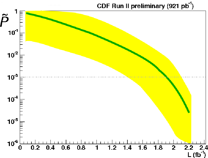
3.4 Summary of first round with 1 fb-1
In the first round of this analysis, with 927 pb-1, a complete Standard Model background estimate has been obtained and compared with data in 344 populated exclusive final states and 16,486 relevant kinematic distributions. Consideration of exclusive final state populations yields no statistically significant () discrepancy after the trials factor is accounted for. Quantifying the difference in shape of kinematic distributions using the Kolmogorov-Smirnov statistic, significant discrepancies are observed between data and Standard Model prediction. These discrepancies are believed to arise from mismodeling of the parton shower and intrinsic , and represent observables for which a QCD-based understanding is highly motivated. None of the shape discrepancies highlighted motivates a new physics claim.
A further systematic search (Sleuth) for regions of excess on the high- tails of exclusive final states has been performed, representing a quasi-model-independent search for new electroweak scale physics. A measure of interest rigorously accounting for the trials factor associated with looking in many regions with few events is defined, and used to quantify the most interesting region observed in the CDF Run II data. No region of excess on the high- tail of any of the Sleuth exclusive final states surpasses the discovery threshold.
Although this result of course can not prove that no new physics is hiding in the studied data, this search is the most encompassing test of the Standard Model at the energy frontier.
Chapter 4 Update with 2 fb-1
This analysis was conducted in two rounds: first with 1 fb-1 of data, and then with 2 fb-1. The first round was presented in Chapter 3. This chapter summarizes the second round.
4.1 Overview
Four separate statistics are employed to search for evidence of new physics. These statistics are
- •
a difference between the number of observed and predicted events in individual exclusive final states;
- •
a difference in distribution shape between data and Standard Model prediction in a variety of kinematic variables;
- •
an excess of data in the large tail of exclusive final states; and
- •
a local excess (bump) in some invariant mass distribution, reflecting possibly a new resonance.
The next sections discus these statistics: Sec. 4.2 is about the normalization and shape statistics, Sec. 4.3 about the statistic, and Sec. 4.4 about the mass bump statistic. Conclusions are provided in Sec. 4.5.
4.2 Vista
Conceptually, Vista in the second round of analysis is the same as in the first.
4.2.1 Object identification
The particle identification criteria used in this analysis are the same as in the first round, except for the following changes:
- •
Changed previously suboptimal conversion filter to the standard one. In the previous version, we required each lepton candidate to not have within another track of opposite sign. The neighbor track was counted only if it had GeV. In this version, we make no transverse momentum requirement on the candidate neighbor tracks. This change reduces significantly the rate for jets and photons to fake electrons, since both fakings involve conversions.
- •
For plug electrons we now require the presence of a good quality PES cluster11 1 Variables and need to be defined and less than 0.65., and that the PHX track matches to the electromagnetic cluster to within . This reduces the rate of jets faking electrons in the region .
- •
For CMUP muons, we require CMU the distance between a stub and the track extrapolation () to be less than 7 cm, instead of 3 cm. This follows a change in the standard muon identification criteria used by the experiment.
- •
For taus, the momentum is now taken from the calorimeter rather than visible momentum (track momentum plus s). The minimum seed track requirement has been increased to 10.5 GeV, reflecting a change in online trigger criteria. We also added an additional muon veto cut requiring that the calorimter over seed track be greater than 0.5, inconsistent with a minimum ionizing particle.
- •
For plug photons, we apply the fiducial cut .
Tables with identification criteria for all objects can be found in Appendix B.2.
4.2.2 Event selection
The following criteria are used to keep events of interest. Single-object criteria accept events containing:
- •
a central electron with GeV, or
- •
a plug electron with GeV, or
- •
a central muon with GeV, or
- •
a central photon with GeV, or
- •
a central or plug photon with GeV, or
- •
a central jet or -tagged jet with GeV, or
- •
a central -tagged jet with GeV (prescaled by the online jet20 trigger), or
- •
a central jet or -tagged jet with GeV (prescaled by 10 in addition to the online jet20 trigger prescale).
Di-object criteria keep events containing:
- •
one electron plus one electron or photon with and GeV, or
- •
a central or plug electron with GeV and a central tau with GeV, or
- •
a central muon with GeV and a central or plug photon with GeV, or
- •
a central muon with GeV and a central -tagged jet with GeV, or
- •
two taus with and GeV, or
- •
a central or plug photon with GeV and a central tau with GeV, or
- •
one central photon with GeV and one other central or plug photon with GeV, or
- •
a central photon with GeV and a central -tagged jet with GeV, or
- •
a central jet or -tagged jet with GeV and a central tau with GeV (prescaled by the online jet20 trigger), or
- •
a central jet with GeV and a central -tagged jet with GeV (prescaled by the online jet20 trigger), or
- •
two central muons with GeV, or
- •
one central electron and one central muon with GeV, or
- •
one central electron with GeV and one central tau with GeV, or
- •
one plug electron with GeV and one central muon with GeV, or
- •
one central muon with GeV and one central tau with GeV.
Tri-object criteria keep events containing:
- •
a central or plug photon with GeV and two central taus with GeV, or
- •
a central or plug photon with GeV and two central -tagged jets with GeV, or
- •
a central or plug photon with GeV, a central tau with GeV, and a central -tagged jet with GeV, or
- •
one -tagged jet with GeV and two more -tagged jets with GeV, or
- •
one central muon with GeV and two other central or plug muons with GeV.
Additional special criteria accept events containing:
- •
one central or plug electron with GeV, missing transverse momentum greater than GeV, and two or more jets or central -tagged jets with GeV, or
- •
one central muon with GeV, missing transverse momentum greater than GeV, and two or more jets or central -tagged jets with GeV.
The above criteria are set by the requirements that the corresponding Standard Model prediction can be generated with enough Monte Carlo event to have weights , and that trigger efficiencies can be treated as roughly independent of object , while keeping as many potentially interesting events as possible.
Explicit online trigger paths are no longer required. CDF specific details are provided in Sec. B.1.
4.2.3 Event generation
Here are summarized changes made to our Monte Carlo event generation since the first round of analysis.
- •
A number of electroweak samples changed to use the newest (Gen6) CDFsim version. They include (the Stntuple sample names are given in parentheses): Pythia (we0sfe, we0sge, we0she), Pythia (we0s8m, we0s9m), Pythia (we0s9t, we0sat), Pythia (ze1s6d, ze1sad, ze0scd, ze0sdd, ze0sed, ze0see), Pythia (ze1s9m, ze0sbm, ze0scm, ze0sdm, ze0sem), Pythia (ze0s8t, ze0sat), Pythia WW (we0sbd, we0sgd), Pythia WZ (we0scd), Baur (re0s28, re0s48), Baur (re0s29, re0s49), Baur (re0s1a, re0s4a).
- •
A low mass Drell-Yan sample was added with going down to 10 GeV (zx0sde, zx0sdm)
- •
We switched from using the Mrenna matched W+jets sample to the standard Top Group Alpgen W+jets samples: +jets (ptopw0, ptopw1, ptop2w, ptop3w, ptop4w), +jets (ptopw5, ptopw6, ptop7w, ptop8w, ptop9w), +jets (utopw0, utopw1, utop2w, utop3w, utop4w).
- •
We switched from using MadEvent W+bbar to the standard Top Group W+bbar sample: +bb+jets (btop0w, btop1w, btop2w), +bb+jets (btop5w, btop6w, btop7w).
Table 4.1 summarizes the contributions from each Monte Carlo sample.
Dataset           Process                   Weights * Number  =  Total weight  |  Dataset          Process                   Weights * Number  =  Total weight
-----------       ----------------          -------   ------     ------------  |  -----------      ----------------          -------   ------     ------------
pyth_jj_000       Pythia jj 0<pT<10         1700           1         1720.13   |  alpgen_muvmj     Alpgen W(-> mu v) j           0.3    281072        83565.2
pyth_jj_010       Pythia jj 10<pT<18         330          74        24368.4    |  ut0s2w           Alpgen W(-> tau v)+jets       0.29     5230         1537.91
pyth_pj_008       Pythia j gamma 8<pT<12      86           5          430.59   |  mad_vtvt-a       MadEvent Z(->vv) gamma        0.27      136           37.22
mrenna_mu+mu-     MadEvent Z(-> mu mu)        29         220         6478.07   |  mad_veve-a       MadEvent Z(->vv) gamma        0.27      135           36.91
pyth_jj_090       Pythia jj 90<pT<120         22        2064        45825.1    |  we0s9t           Pythia W(-> tau v)            0.26    66024        17105.3
pyth_pj_012       Pythia j gamma 12<pT<22     21        1970        41809.2    |  ut0sw1           Alpgen W(-> tau v)+jets       0.24    27785         6634.6
pyth_jj_018       Pythia jj 18<pT<40          18       24807       444683      |  pyth_pp          Pythia gamma gamma            0.23    25552         5783.53
alpgen_eve        Alpgen W(->e v)             12        5807        68133.2    |  ze1s6d           Pythia Z(->ee)                0.22   484676       106397
mad_vtvt-j        MadEvent Z(->vv) j          11           3           32.25   |  mad_e+e-b-b      MadEvent Z(->ee) bb           0.22     1028          224
mad_veve-j        MadEvent Z(->vv) j          11           3           32.01   |  alpgen_evejj     Alpgen W(->e v) jj            0.21   175665        37470.9
mrenna_e+e-       MadEvent Z(->ee)            10        5965        60080.4    |  re0s28           Baur W(->ev) gamma            0.21    22074         4698.99
alpgen_muvm       Alpgen W(-> mu v)            9.9      4483        44217.8    |  alpgen_muvmjj    Alpgen W(-> mu v) jj          0.2    112546        22201.2
pyth_jj_120       Pythia jj 120<pT<150         8.2      3291        27109.7    |  ztopcz           Pythia ZZ                     0.19      588          110.12
pyth_bj_010       Pythia bj 10<pT<18           7.7        96          739.91   |  stelzer_Zaj      stelzer_Zaj                   0.18     1592          288.68
pyth_jj_060       Pythia jj 60<pT<90           6.7     25300       170628      |  mad_aajj         MadEvent jj gamma gamma       0.18     7825         1406.23
mrenna_mu+mu-j    MadEvent Z(-> mu mu) j       6.6      3209        21131      |  mad_mu+mu-b-b    MadEvent Z(-> mu mu) bb       0.17      624          109.01
pyth_jj_040       Pythia jj 40<pT<60           5       87760       440765      |  mad_e+e-jj       MadEvent Z(->ee) jj           0.17      775          134.36
pyth_jj_200       Pythia jj 200<pT<300         3.4     73024       249462      |  re0s29           Baur W(-> mu v) gamma         0.17    19972         3454.5
mad_veve-a_f      MadEvent Z(->vv) gamma       3.4        13           44.3    |  re0s1a           Baur W(-> tau v) gamma        0.17     2823          467.2
ut0sw0            Alpgen W(-> tau v)+jets      3.2       643         2065.45   |  pyth_jj_300      Pythia jj 300<pT<400          0.14   103800        14883.7
pyth_pj_022       Pythia j gamma 22<pT<45      3       31039        93761.3    |  mad_aaa_f        MadEvent gamma gamma gamma    0.14       52            7.4
pyth_jj_150       Pythia jj 150<pT<200         2.7     59183       162311      |  cosmic_j_hi      Cosmic (jet100)               0.12    36674         4487.59
we0sfe            Pythia W(->e v)              2.4    381263       921806      |  pyth_bj_040      Pythia bj 40<pT<60            0.12   160713        18850
cosmic_j_lo       Cosmic (jet20)               2.3       122          277.24   |  mrenna_e+e-jjj   MadEvent Z(->ee) jjj          0.11    23995         2667.48
cosmic_ph         Cosmic (photon_25_iso)       1.9      2694         4989.53   |  ze0s8t           Pythia Z(-> tau tau)          0.093   15030         1400.09
pyth_pj_080       Pythia j gamma 80<pT         1.5     18378        28063.9    |  pyth_bj_200      Pythia bj 200<pT<300          0.081  254807        20679.8
mrenna_e+e-j      MadEvent Z(->ee) j           1.5     28104        40784.4    |  hewk03           MadEvent Z(->ee) gamma        0.081   70476         5709.75
pyth_pj_045       Pythia j gamma 45<pT<80      1.4     82466       117398      |  mad_aaa          MadEvent gamma gamma gamma    0.08       73            5.82
mrenna_mu+mu-jj   MadEvent Z(-> mu mu) jj      1.3      4146         5503.42   |  wenubb0p         Alpgen W(->e v) bb            0.075   41459         3105.72
mad_veve-j_f      MadEvent Z(->vv) j           1.2         6            7.23   |  wmnubb0p         Alpgen W(-> mu v) bb          0.075   26067         1952.18
pyth_bj_018       Pythia bj 18<pT<40           1.2     15659        18163.1    |  zx0sem           Pythia Z(-> mu mu) (m_Z<20)   0.075      45            3.37
mad_e+e-          MadEvent Z(->ee)             1         520          540.85   |  zx0see           Pythia Z(->ee) (m_Z<20)       0.074      73            5.37
stelzer_l+l-j     stelzer_l+l-j                0.92      668          615.62   |  wenubb1p         Alpgen W(->e v) bb j          0.072   14111         1021.01
mrenna_e+e-jj     MadEvent Z(->ee) jj          0.92    11258        10307.9    |  wmnubb1p         Alpgen W(-> mu v) bb j        0.072    8426          609.28
mad_mu+mu-        MadEvent Z(-> mu mu)         0.89       82           72.79   |  hewk04           MadEvent Z(-> mu mu) gamma    0.072    2032          145.67
pyth_bj_060       Pythia bj 60<pT<90           0.87    10723         9348.26   |  overlay          Overlaid events               0.071   11118          794.91
mad_vtvt-a_f      MadEvent Z(->vv) gamma       0.84       38           32      |  pyth_jj_400      Pythia jj 400<pT              0.068   13153          894.13
pyth_bj_090       Pythia bj 90<pT<120          0.84     2374         1990.9    |  alpgen_evejjj    Alpgen W(->e v) jjj           0.068   92857         6284.23
mad_vtvt-j_f      MadEvent Z(->vv) j           0.81        5            4.07   |  alpgen_muvmjjj   Alpgen W(-> mu v) jjj         0.066   55704         3693.97
stelzer_Waj       MadEvent W(->l v)j gamma     0.69     1637         1124.5    |  ttop0z           Herwig ttbar                  0.065   30518         1983.29
pyth_bj_120       Pythia bj 120<pT<150         0.67     2848         1903.72   |  ut0s3w           Alpgen W(-> tau v)+jets       0.063    4458          281.47
mad_aaj           MadEvent j gamma gamma       0.52      559          289.03   |  ze0sat           Pythia Z(-> tau tau)          0.063   22882         1438.37
we0s8m            Pythia W(-> mu v)            0.49  1.2908e+06    630955      |  wmnubb2p         Alpgen W(-> mu v) bb jj       0.054    3529          189.63
pyth_bj_150       Pythia bj 150<pT<200         0.45    28272        12593.5    |  wenubb2p         Alpgen W(->e v) bb jj         0.054    6075          325.2
mrenna_mu+mu-jjj  MadEvent Z(-> mu mu) jjj     0.44     3435         1498.33   |  we0scd           Pythia WZ                     0.053    2890          154.28
mad_e+e-j         MadEvent Z(->ee) j           0.39      735          286.71   |  we0sbd           Pythia WW                     0.048    2839          136.4
alpgen_evej       Alpgen W(->e v) j            0.35   398558       140544      |  we0sgd           Pythia WW                     0.048    2567          122.92
we0sat            Pythia W(-> tau v)           0.35    49543        17155.3    |  alpgen_evejjjj   Alpgen W(->e v) jjjj          0.027   41696         1123.15
mad_mu+mu-j       MadEvent Z(-> mu mu) j       0.34      494          166.35   |  alpgen_muvmjjjj  Alpgen W(-> mu v) jjjj        0.024   27099          662.36
mad_mu+mu-jj      MadEvent Z(-> mu mu) jj      0.32     1681          532      |  ut0s4w           Alpgen W(-> tau v)+jets       0.022    2551           56.84
ze1s9m            Pythia Z(-> mu mu)           0.3    370995       110522      |  Total:                                                           4.36864e+06
| Code | Category | Explanation | Value | Error | Error(%) |
|---|---|---|---|---|---|
| 0001 | luminosity | CDF integrated luminosity | 1990 | 50 | 2.6 |
| 0002 | -factor | cosmic_ph | 0.83 | 0.05 | 6.0 |
| 0003 | -factor | cosmic_j | 0.192 | 0.006 | 3.1 |
| 0004 | -factor | 11j photon+jet(s) | 0.92 | 0.04 | 4.4 |
| 0005 | -factor | 12j | 1.26 | 0.05 | 4.0 |
| 0006 | -factor | 13j | 1.61 | 0.08 | 5.0 |
| 0007 | -factor | 14j+ | 1.94 | 0.16 | 8.3 |
| 0008 | -factor | 20j diphoton(+jets) | 1.6 | 0.08 | 5.0 |
| 0009 | -factor | 21j | 2.99 | 0.17 | 5.7 |
| 0010 | -factor | 22j+ | 1.2 | 0.09 | 7.5 |
| 0011 | -factor | W0j W (+jets) | 1.38 | 0.03 | 2.2 |
| 0012 | -factor | W1j | 1.33 | 0.03 | 2.3 |
| 0013 | -factor | W2j | 1.99 | 0.05 | 2.5 |
| 0014 | -factor | W3j+ | 2.11 | 0.09 | 4.3 |
| 0015 | -factor | Z0j Z (+jets) | 1.39 | 0.028 | 2.0 |
| 0016 | -factor | Z1j | 1.23 | 0.04 | 3.2 |
| 0017 | -factor | Z2j+ | 1.02 | 0.04 | 3.9 |
| 0018 | -factor | 2j 150 dijet | 1.003 | 0.027 | 2.7 |
| 0019 | -factor | 2j 150 | 1.34 | 0.03 | 2.2 |
| 0020 | -factor | 3j 150 multijet | 0.941 | 0.025 | 2.7 |
| 0021 | -factor | 3j 150 | 1.48 | 0.04 | 2.7 |
| 0022 | -factor | 4j 150 | 1.06 | 0.03 | 2.8 |
| 0023 | -factor | 4j 150 | 1.93 | 0.06 | 3.1 |
| 0024 | -factor | 5j low | 1.33 | 0.05 | 3.8 |
| 0025 | -factor | 1b2j 150 | 2.22 | 0.11 | 5.0 |
| 0026 | -factor | 1b3j 150 | 2.98 | 0.15 | 5.0 |
| 0027 | misId | p(ee) central | 0.978 | 0.006 | 0.6 |
| 0028 | misId | p(ee) plug | 0.966 | 0.007 | 0.7 |
| 0029 | misId | p() CMUP+CMX | 0.888 | 0.007 | 0.8 |
| 0030 | misId | p() central | 0.949 | 0.018 | 1.9 |
| 0031 | misId | p() plug | 0.859 | 0.016 | 1.9 |
| 0032 | misId | p(bb) central | 0.978 | 0.021 | 2.1 |
| 0033 | misId | p(e) plug | 0.06 | 0.003 | 5.0 |
| 0034 | misId | p(qe) central | 7.09 | 1.9 | 2.7 |
| 0035 | misId | p(qe) plug | 0.000766 | 1.2 | 1.6 |
| 0036 | misId | p(q) | 1.14 | 6 | 5.2 |
| 0037 | misId | p(b) | 3.3 | 1.1 | 33.0 |
| 0038 | misId | p(jb) 25 | 0.0183 | 0.0002 | 1.1 |
| 0039 | misId | p(q) | 0.0052 | 0.0001 | 1.9 |
| 0040 | misId | p(q) central | 0.000266 | 1.4 | 5.3 |
| 0041 | misId | p(q) plug | 0.00048 | 6 | 12.6 |
| 0042 | trigger | p(etrig) plug, 25 | 0.86 | 0.007 | 0.8 |
| 0043 | trigger | p(trig) CMUP+CMX, 25 | 0.916 | 0.004 | 0.4 |
Specific modifications to the correction model implemented since the first round are described here.
- •
The integrated luminosity of the data sample considered has increased from 927 to 1990 pb-1. The integrated luminosity correction factor has been adjusted accordingly.
- •
Events from more recent data have been included in the high- jet and photon non-collision backgrounds. For events with GeV and at least two jets of GeV and no objects of other kinds, we require the of the jet with the second largest to be greater than 75 GeV. This cut is to clean multijet samples of events where the second jet comes from the underlying event but the first jet is due to a cosmic ray. Such events are not modeled well by our cosmic background, which comprises events required to have less than three tracks; this requirement reduces the fraction of such cosmic + jet(s) events relative to the data sample, where more than three tracks are required. As a result of these changes, the cosmic_ph and cosmic_j correction factors have been readjusted.
- •
It was recognized that in the previous version of the analysis we had been using a suboptimal filter for conversion electrons. This filter has been updated and now yields a substantially reduced rate for jets faking electrons via fragmentation to a leading .
- •
In order to accommodate the ditau trigger, which in recent data requires a seed track with GeV, and recognizing our concentration on the identification of single-prong taus, the track requirement for taus has been increased to 10.5 GeV. The fake rate and its dependence on have been adjusted accordingly.
- •
In order to address questions regarding the fake rate and its consistent simultaneous application to many final states, the measurement of tau is now based on the energy deposited in the calorimeter.
- •
In order to address questions regarding the fake rate and its consistent simultaneous application to multijet final states with large and small , a monotonically decreasing dependence of the fake rate on the generated summed scalar transverse momentum has been imposed.
- •
In the implementation of the fake rates , , and , jets from a parent or quark now only fake positively charged and leptons (and positrons rather than electrons at a ratio of 2:1), and jets from a parent or quark now only fake negatively charged and leptons (and electrons rather than positrons at a ratio of 2:1).
- •
The ditau trigger, which turned on roughly 300 pb-1 into Run II, has now been live for a greater fraction of the total integrated dataset. The effective ditau trigger effeciency has been adjusted accordingly.
- •
A fake rate has been introduced.
- •
The dependence of the fake rate and has been adjusted.
- •
The and dependence of the fake rate and has been adjusted to take into account more geometric features of the detector including the calorimeter cracks at of 0 and 1.1.
- •
The efficiency for reconstructing a jet as a non--tagged jet has been reduced from 1 to 1-.
- •
Separate -factors have been introduced for heavy flavor multijet production for the high- sample. Specifically, a new -factor has been introduced for events with at least one heavy flavor jet and three jets in total, with . Another -factor has been introduced for events with at least one heavy flavor jet and four or more jets in total, with . They are listed in the table of correction factors 4.2 as 1b2j and 1b3j.
4.2.4 Results
| Final State | Data | Background | ||
|---|---|---|---|---|
| b | ||||
| b2j high- | ||||
| 2j low- | ||||
| 3j low- | ||||
| 2j | ||||
| j | ||||
| j | ||||
| 2j | ||||
| 2bj low- | ||||
| j low- | ||||
| 2b2j low- | ||||
| b | ||||
| 2b | ||||
| 8j | ||||
| 7j | ||||
| 6j | ||||
| 5j | ||||
| 4j high- | ||||
| 4j low- | ||||
| 4j | ||||
| 4j high- | ||||
| 4j low- | ||||
| 4j high- | ||||
| 4j | ||||
| 4j | ||||
| 4j | ||||
| 4j | ||||
| 4j | ||||
| 4j | ||||
| 3j high- | ||||
| 3j low- | ||||
| 3j | ||||
| 3j high- | ||||
| 3j high- | ||||
| 3j low- | ||||
| 3j | ||||
| 3j | ||||
| 3j | ||||
| 3j | ||||
| 3j | ||||
| 3j | ||||
| 3j | ||||
| 3j | ||||
| 3b2j | ||||
| 3bj | ||||
| 3b | ||||
| 2j high- | ||||
| 2j low- | ||||
| 2j | ||||
| 2j | ||||
| 2j | ||||
| 2j high- | ||||
| Final State | Data | Background | ||
|---|---|---|---|---|
| 2j high- | ||||
| 2j low- | ||||
| 2j | ||||
| 2j | ||||
| 2j | ||||
| 2j | ||||
| 2j | ||||
| 2j | ||||
| 2j | ||||
| 2j | ||||
| 2j | ||||
| 2j | ||||
| 2j | ||||
| j | ||||
| 2b high- | ||||
| 2b low- | ||||
| 2b3j low- | ||||
| 2b2j high- | ||||
| 2b2j high- | ||||
| 2b2j | ||||
| 2b2j | ||||
| 2b2j | ||||
| 2b | ||||
| 2bj high- | ||||
| 2bj high- | ||||
| 2bj | ||||
| 2bj | ||||
| 2b2j | ||||
| 2b2j | ||||
| 2b | ||||
| 2bj | ||||
| 2bj | ||||
| 2b | ||||
| j | ||||
| j | ||||
| j high- | ||||
| j | ||||
| j high- | ||||
| j | ||||
| j | ||||
| j | ||||
| j | ||||
| j | ||||
| j | ||||
| j | ||||
| j | ||||
| j | ||||
| Final State | Data | Background | ||
|---|---|---|---|---|
| j | ||||
| j | ||||
| j | ||||
| j | ||||
| 4j | ||||
| 4j | ||||
| 4j | ||||
| 3j | ||||
| 3j | ||||
| 3j | ||||
| 3j | ||||
| 2j | ||||
| 2j | ||||
| 2j | ||||
| 2j | ||||
| 2j | ||||
| 2j | ||||
| 2j | ||||
| j | ||||
| j | ||||
| j | ||||
| j | ||||
| j | ||||
| j | ||||
| j | ||||
| j | ||||
| j | ||||
| j | ||||
| j | ||||
| j | ||||
| 4j | ||||
| 3j | ||||
| 2j | ||||
| 2j | ||||
| 2j | ||||
| j | ||||
| j | ||||
| j | ||||
| b6j | ||||
| b5j | ||||
| b4j high- | ||||
| b4j low- | ||||
| b3j high- | ||||
| b3j low- | ||||
 |
 |
The global fit , described in Sec. 3.2.5, was in the second round , from 335 bins, plus a 28.4 from external constraints. It is obviously a very large , even more unlikely than it was in the first round of the analysis, indicating that deviations from the fit are clearly non-statistical, but due to systematic imperfections in our Standard Model implementation. Higher statistics exacerbate systematic imperfections.
Table 4.3 shows the comparison of CDF Run II 2 fb-1 data to Standard Model prediction. All events have been partitioned in exclusive final states. The number of events observed is compared to the number expected from the Standard Model, taking into account the uncertainty due to finite Monte Carlo statistics, and the trials factor due to examining 399 final states. The final states are ordered in decreasing discrepancy.
No final state is found to have a population discrepancy that is considered significant after accounting for the trials factor. The largest population discrepancy is a 2.7 deficit (including trials factor) observed in final state . Fig. 4.1 summarizes in a histogram the distribution of discrepancies observed in final state populations. Qualitatively, shape discrepancies give us the same information we had in the first round of the analysis.
Discrepant distributions are flagged using the Kolmogorov-Smirnov (KS) statistic. 22 2 The KS statistic is defined in terms of the cumulative distributions of two populations. Given a particular distribution, such as the invariant mass mass(j1,j2) of the two jets in the 1e+2j1pmiss final state, the Standard Model prediction and the data are both normalized to unit integral, and the cumulative distributions are drawn. The maximal separation of the two cumulative distributions is the KS statistic, a number between 0 and 1. This statistic can be translated into a probability for the data to have been pulled from the Standard Model distribution, with the translation depending only on the value of the statistic and the number of data events. This KS probability can then be converted into units of standard deviations by solving . Fig. 4.1 shows a histogram of the disagreement seen in all kinematic distributions. 19,650 distributions are considered in 2 fb-1, and 559 are found to have a significant disagreement. However, as in the first round with 1.0 fb-1, no indication of new physics is found amongst these discrepant distributions; all are attributed to the “3-jet effect”, difficulties with intrinsic or residual coarseness of the correction model.
Evolution of the Vista Global Comparison since 1 fb-1
| Final State | Data | Background | ||
|---|---|---|---|---|
| 4j | ||||
| 4j | ||||
| 4j | ||||
| 4b4j | ||||
| 4b2j | ||||
| 4b | ||||
| 3j | ||||
| 3j | ||||
| 3j | ||||
| 3b4j | ||||
| 3b3j | ||||
| 3b2j | ||||
| 3b2j | ||||
| 3b | ||||
| 3bj | ||||
| 3bj | ||||
| 3bj | ||||
| 3b | ||||
| 2j | ||||
| 2j | ||||
| 2b6j | ||||
| Final State | Data | Background | ||
|---|---|---|---|---|
| 2b | ||||
| 2bj | ||||
| 2bj | ||||
| 2b | ||||
| 2b | ||||
| j | ||||
| j | ||||
| j | ||||
| j | ||||
| 4j | ||||
| 4j | ||||
| 4j | ||||
| 4j | ||||
| 3j | ||||
| j | ||||
| j | ||||
| 2j | ||||
| j | ||||
| Final State | Data | Background | ||
|---|---|---|---|---|
| b6j | ||||
| b4j | ||||
| b3j | ||||
| b2j | ||||
| b2j | ||||
| b | ||||
| b | ||||
| b | ||||
| b | ||||
| bj | ||||
| bj | ||||
| b3j | ||||
| b3j | ||||
| b | ||||
| b2j | ||||
| b2j | ||||
| b2j | ||||
| b | ||||
| b | ||||
| bj | ||||
Table 4.4 displays the Vista final states which newly appeared in the present analysis. A large number involve b-jets; this is a result of changes in our offline event selection criteria, which now accept more events containing b-tagged jets (previously events with a leading b-jet with were prescaled offline by a factor of 10; we also introduced a new tri-b offline selection).
There are also 11 final states which were populated in the 1.0 fb-1 analysis, but are not now: 1b1e+3j1tau- 1b3j2ph 1e+ 1e+1e-1ph1tau+ 1e+3j2ph 1j1pmiss2tau+ 1j3ph 2b2ph 3j1mu+1pmiss1tau+ 3j1pmiss1tau+1tau- 1b1e+3j1ph1pmiss These events were generally found to contain an object (usually a or plug photon) which now fails our tighter identification requirements.
A final reason for the increase of Vista final states from 344 in 1.0 fb-1 to 399, is that jet-tau final states have been divided into high- and low- states.
The 3j and 2j final states remain among the ‘top ten’ most discrepant states, but their significance has decreased compared to the first round. The improvement in agreement was achieved after slight changes in modeling jets faking taus in events with large activity. Other final states from the first round’s top ten now exhibit zero discrepancy (after accounting for the trials factor). We attribute this to a combination of general improvements in modeling and statistical fluctutations.
4.3 Sleuth
Sleuth algorithm was not modified in the second round.
4.3.1 Results
 |
 |
 |
 |
 |
 |

The most interesting final states highlighted by Sleuth are shown in Fig. 4.2. The region chosen by Sleuth is shown by the (blue) arrow, extending up to infinity. CDF Run II data are shown as filled circles; Standard Model prediction is shown as a histogram. Sleuth final state labels are in the upper left corner of each panel. The number at upper right in each panel is , the fraction of hypothetical similar experiments in which something as interesting as the region shown would be seen in this final state. The inset in each panel shows an enlargement of the region selected by Sleuth, together with the number of events (SM) predicted by the Standard Model in this region, and the number of data events () observed in that region.
The distribution of for the final states considered by Sleuth in the CDF Run II data is shown in Fig. 4.3.
In these CDF data, Sleuth finds . This is sufficiently far above the Sleuth discovery threshold of that no discovery claim can be made on the basis of Sleuth for 2 fb-1.
Study of Same-Sign Sleuth States
The top Sleuth final states appear a common trend to involve same-sign leptons. We first consider the 2nd and 3rd Sleuth final states, which both contain same-sign electron and muon, significant missing energy, and varying numbers of jets. The relevant Vista final states are:
| Final State | data | background |
|---|---|---|
| 31 | 29.9 1.6 | |
| 16 | 9.2 1.9 | |
| 6 | 1.7 1.2 | |
| 0 | 0.26 0.07 |
The primary backgrounds for all these final states are similar, although the relative proportions vary with the number of reconstructed jets. The three main backgrounds are: +jets, with a jet faking the electron; +jets, where 1 is not reconstructed, creating missing energy, and a jet fakes the electron; and (+jets), where the photon fakes the electron.
All these processes involve real muons – there is no significant Standard Model contribution to these final states from fake muons. Therefore we can discard any explanation for the excess in data which involves charge assignment to muons faked by jets.
We can be confident that the charge-sign of a real muon is well-measured by the CDF tracking system. The curvature resolution of the chamber is cm-1. The curvature corresponding to a track with momentum of 100 GeV/ is cm-1. The sign of the curvature of such a track, and hence the charge of such a particle, is thus typically determined with a significance of better than five standard deviations [81]. Vista supports this conclusion, since we reconstruct 25,000 events but only a single event (and even then, the invariant mass is 150 GeV, making it unlikely to be a decay with wrong charge-reconstruction).
We can assume the muon charge is correct therefore, and focus on the electron. This is a fake electron from a jet. This fake rate is well-determined from the electron+jet(s) events, and similarly the -factors for the boson+jets processes are well-determined from other final states. We expect the contribution from these processes to these particular final states to therefore be accurate. Indeed, the most populous state 1e+1mu+1pmiss is well described, and the mild excesses seen by Sleuth arise from the 1e+1j1mu+1pmiss and 1e+2j1mu+1pmiss final states. Examination of the kinematic distributions from thse final states yields nothing further (the electron distributions for these final states are shown in Figs. 4.4 and 4.5), so, following the above reasoning and given that the effect is not statistically very signficant, we ascribe the presence of these two states towards the top of Sleuth’s list as likely just due to a fluctuation.


The 1st Sleuth final state 1e+1mu+ also has same sign electron and muon, but no missing energy, and 0 or 1 jets. The potentially relevant Vista final states are:
| Final State | data | background |
|---|---|---|
| 45 | 28.5 1.8 | |
| 13 | 8.2 2 | |
| 2 | 2.6 1.6 | |
| 2 | 0.6 1.2 |
So only the data excess in needs any potential investigation for evidence of Standard Model background mismodeling. The largest background is from +jets, with one muon lost and a jet faking an electron. As explained earlier, this process is well-constrained and cannot explain the excess in data.
The next largest background is , with one decaying to an electron and the other to a muon. As discussed above, we trust the muon charge, so the electron must be reconstructed with the wrong charge. For central electrons, this occurs at a rate on the order of 1 in , through electron bremstrahlung to a photon with an asymmetric conversion that half the time results in an opposite charge electron, and therefore is too small to play a role here. For plug electrons, however, the track charge has a false-reconstruction rate of order 10% [82]. Fig. 4.6 shows the of the electron, and we indeed observe that the contribution is almost entirely in the plug. However, Fig. 4.7, which shows electron for the 2e+ final state (dominated by real electrons from with phoenix track charge mis-assignment), demonstrates that this charge misidentification is quite well modeled – there is certainly no room for the factor of two increase that would be needed to explain the data excess. The only other large background is from QCD dijet events where both electron and muon are fakes. Both of these total fake rates are very well constrained from the electron+jets(s) and muon+jet(s) final states, so the only possible flexibility is in the charge assignment to the fakes, which would shift background events between the 1e+1mu+ and 1e+1mu- final states. However, with our current modeling, this process contributes an approximately equal number of expected events () to each of these states. It is implausible to argue that the combination of QCD Feynman diagrams and faking mechanisms could be such as to significantly anti-correlate the fake electron and muon charge signs, so this cannot contribute to the data excess. In conclusion, after examining the possibilities and reminding ourselves that the similar final states but with additional jets are actually well described, we have no explanation for this excess other than a statistical fluctuation.


The 5th most discrepant state in Sleuth is . Since Sleuth combines electrons and muons, the relevant Vista final states are:
| Final State | data | background |
|---|---|---|
| 36 | 17.2 1.7 | |
| 11 | 8.3 1.5 | |
| 15 | 12 2 | |
| 8 | 9.4 3.1 |
One sees that the excess comes only from . This is actually among most discrepant final states in Vista, with a significance of 1.4 after accounting for the trials factor. The primary background is +jet, where the jet ends up faking a with the same charge as the electron. This is rarer than the other case where the fake has opposite sign to the electron. However, we appear to be modeling this process quite well, because it equally applies in the case when the decays to muon and neutrino, and Vista predicts those final states correctly. We believe the excess in is therefore likely just a fluctuation.
In conclusion, although the top Sleuth states all involve same-sign leptons, we find no explanation that can simultaneously account for all. More data would help us see to what extent this is mismodeling, and to what statistical fluctuation.
Evolution of the Top Sleuth Final States from 1 fb-1
The 1bb final state which was at the top of the list of Sleuth discrepancies has now gone down the list. The reason is that the region selected previously had been selected based on a relatively small excess in a particular region of . Doubling the data caused that region to exceed the upper limit of 10,000 events. This upper limit is designed to reject excesses found in regions of high statistics where even a small systematic error would cause Sleuth to give a large discrepancy.
The discrepancy in the final state, which is dominated by cosmic events, has been corrected by the additional quality criteria cuts on the cosmic background.
The 3rd, 4th and 6th most discrepant Sleuth final states from the first round were same sign dilepton final states. These final states have become more discrepant in this round of the analysis as discussed in Sec. 4.3.1.
The 5th most discrepant Sleuth final state from the first round of the analysis was the . Then, we a major background contribution was missing, , which has been added.
The remaining discrepancies were all corrected either by improving the background modelling, or were simply fluctuations.
4.3.2 Sensitivity
For the 2 fb-1 analysis, we have performed an additional test of the sensitivity of Sleuth to Standard Model single top production.
| Final State | Events | Acceptance (%) |
|---|---|---|
| 5149 | 5.1 | |
| 3231 | 3.2 | |
| 1977 | 2.0 | |
| 298 | 0.3 | |
| 219 | 0.2 | |
| 128 | 0.1 | |
| 109 | 0.1 | |
| 96 | 0.1 | |
| 59 | 0.1 | |
| 41 | 0.0 |
| cost | Final state | |
|---|---|---|
| 3600 | 0.0009669 | |
| 4800 | 0.0003004 | |
| 3800 | 0.0002808 | |
| 3600 | 0.0008754 | |
| 3600 | 0.0002843 | |
| 3800 | 0.0007113 | |
| 5000 | 0.0007072 | |
| 3800 | 0.0003327 | |
| 5400 | 0.0003309 | |
| 2800 | 0.0004739 |
 |
 |
This sensitivity test is performed by injecting ‘signal’ single top events into pseudo-data generated from the background. Single top events are obtained from the CDF Top Group Monte Carlo samples stop00 and stop01 (-channel and -channel production respectively), run through our standard event reconstruction. The acceptance for the signal events into Sleuth final states is shown in Table 4.5.
Signal events are added to the pseudo-data in chunks, until Sleuth’s discovery threshold of is reached. To account for random fluctuations, ten such trials are performed and the final result is averaged from all trials. Table 4.6 summarizes the result of each trial.
As expected, Sleuth’s ‘golden’ final state for discovering single top is . The % acceptance into this final state is consistent with the numbers obtained for dedicated single top searches [83]. Note that due to the definition of final states in Sleuth, contains events with 2 or 3 jets, with at least 1 -tag. This merges somewhat the standard single top separation into distinct 2-jet and 3-jet bins, and this is why the background contribution is relatively large.
An example ‘discovery’ is illustrated in Fig. 4.8. This shows the combined background prediction in the absence of signal, and the distribution after adding sufficient signal to trigger Sleuth’s discovery threshold. Fig. 4.9 illustrates the distribution from single top signal relative to the combined background prediction.

The result of this sensitivity test is that Sleuth would be expected to discover single top at the level in 2 fb-1 if it had a cross-section of pb. The Standard Model expected cross-section is 2.86 pb (combined - and -channel). A naive extrapolation therefore leads to an expected luminosity for Sleuth discovery of fb-1.
This conclusion seems perhaps surprising given the effort devoted to sophisticated tools such as Matrix Elements and Neural Networks for dedicated single top searches. The apparent sensitivity of Sleuth stems from the fact that it treats the background as being absolutely fixed. Any addition is therefore considered pure signal, allowing ‘discovery’ of single top with relatively few extra events. In practice this is unrealistic, since alone would find it hard to distinguish between single top production and excess +heavy flavour relative to Alpgen predictions, which have a large uncertainty. In a realistic test, we would probably have to introduce a separate -factor for +heavy flavour, which would swallow up much of the single top signal, since there is no other populous final state that could constrain the W+heavy flavor -factor independently of possible single top contributions. For the dedicated single top searches, the total backgrounds are generally allowed to float, and more sophisticated purely ‘shape-based’ variables are used to discriminate signal from background.
4.4 Bump Hunter
The bump hunter is a new feature added in the second round of this analysis, to enhance the sensitivity of the search to new physics involving narrow mass resonances.
4.4.1 Strategy
The idea is to scan the spectrum of most mass variables with a sliding window. The window needs to vary in width to follow the changing detector resolution. As the window drifts accross a mass distribution, it evaluates the probability that the amount of data therein, or even more, could have emerged by fluctuation from the predicted population. The window where this probability is smallest contains the most interesting local excess of data.
In each final state there are typically several mass variables to scan. On average there are . They include masses of all combinations of reconstructed objects, such as pairs, triplets, or bigger ensembles.
The width of the sliding window equals two times the characteristic mass resolution for the given combination of objects and at the given mass value. Mass uncertainty results from uncertainties about the specific energies and momenta of all objects involved. It is possible to have combinations of four-momenta that result in the same mass, but different mass uncertainties. For example, if a decays to , the mass of that pair will always be close to the nominal GeV, though its resolution will depend on the boost of the decaying . Obviously, each event has a different mass uncertainty, so we need to estimate the characteristic mass resolution at each value of mass and for each mass variable. That characteristic mass resolution will be representative of the mass resolution of the events there. To estimate it, we assume that all objects in the ensemble have equal momentum, negligible mass, and their momenta balance on a plane33 3 If the (equal) momenta are two, to balance they have to be back-to-back. If they are three, they have to be on the same plane, each separated by from its first neighbors. If we have equal, balancing momenta in 3 dimensions, then their angular configurations can be significantly more complicated, as there are many possible arrangements that satisfy the condition of ballance. To avoid such complexity, we choose to constrain all vectors in one plane, and assume the solution where all vectors have separation from their nearest neighbors.. Then, we assign to each involved individual energy the appropriate uncertainty, depending on what object it belongs to, since different objects are measured with different energy resolutions. For electrons and photons, the uncertainty is assumed to be , determined by the electromagnetic calorimeter. For jets and s it is taken to be , determined by the hadronic calorimeter. For (beam constrained) muons it is , determined by the COT track curvature resolution. In cases of transverse mass involving , we assume roughly . We propagate those s corresponding to the members of the ensemble into the system’s total mass. For example, if we want to find the characteristic mass resolution for a triplet at system mass 90 GeV, we have . We assume and the planar configuration with zero net momentum, to obtain that , hence GeV for each object. We use the above formulas for the three different s, keeping in mind the different resolutions for electrons, muons and jets, and then we propagate those uncorrelated uncertainties to the mass, to find GeV.
The step size by which the window drifts equals half a characteristic mass resolution, therefore it varies along the mass spectrum, as the width does too. That way there are no gaps left between consecutive windows. Instead, consecutive windows partly overlap.
Each window comes with two sidebands, extending on each side as far as the window’s width. The region of the spectrum that is scanned is slightly narrower than the whole spectrum’s span (defined as the interval between the highest-mass and the lowest-mass event in both data and background), so that all considered windows have sidebands lying within the spectrum.
As the window drifts along a mass spectrum, its is calculated at each location. That is defined as the Poisson probability that the Standard Model events expected in the window () would fluctuate up to or above the observed data (), i.e. .
A window qualifies as a bump if it satisfies the following criteria:
- •
The central region must contain at least 5 data events.
- •
Both sidebands must be less discrepant than the central region, i.e. both must have larger .
- •
If the background in a sideband is non-zero, then it must have , namely it must not exhibit a significant () discrepancy. If the background is zero, then it must have less than 5 data44 4 This special treatment of the zero-background case is to be able to spot excesses of data that may be isolated at mass values where there is no Standard Model background at all. If we had, for example, 6 events in the central window and 1 event in the sideband, we wouldn’t like this band to disqualify due to having a discrepant sideband..
- •
The above criteria need to hold even when we consider the possible effects of low Monte Carlo statistics in the background. This is explained next.
It can happen to have a great excess of data in the central window, and simultaneously non-discrepant sidebands, but realize that the sidebands contain only a couple of very large-weight events in the Standard Model background. These large-weight events are called “spikes”, and are the result of limited Monte Carlo statistics. That bump would potentially pass all quality criteria, and appear to be statistically significant, but it would be prudent to treat conservatively the presence of spikes in the sidebands, and consider that these Monte Carlo events could easily have been in the central window instead. In that case, the of the central window would be larger (less significant) and the sidebands would have a higher probability to be discrepant, hence the bump could disqualify. Since limited Monte Carlo statistics are a practical limitation, we have to be conservative and eliminate, if necessary, this bump. To do that, we first need to define what we consider as a spike in each sideband, and reevaluate the and the quality of the bump, assuming the spikes from both sidebands transfered into the central window. To define the weight of spikes in a sideband, we look for outliers among the Monte Carlo events, namely for events with significantly larger weights than the average weight of the events in the sideband. We find the average weight and the standard deviation of weights in the sideband, including in the calculation all Monte Carlo events therein. If there is an event whose weight lies beyond 3 standard deviations from the average, then we gradually reduce its weight. As we reduce it, we reevaluate the average and standard deviation of weights. If along its path towards smaller weight it meets another event of same weight, then their weights are bound to be equal from then on, and keep being gradually reduced together. To visualize this process, imagine the axis of weights as an horizontal stretched string, and the weight of each event represented by the position of a tiny bead along this string; the larger the weight, the farther on the right the bead is located. If there are significant outliers, namely beads very far on the right, we start pushing the rightmost bead slowly from right to left, to bring it closer to the others. On its way, the rightmost bead drags with it any beads it meets, since beads can not pass through each other. We stop this reduction of weights when they are all within 3 standard deviations from their average. Then, we compare the total initial weight to the total final weight in the sideband. The difference is weight attributed to spikes. If this difference turns out to be smaller than the largest single weight in the sideband, then we define the latter as spike instead. For the sake of saving time, we do not apply the anti-spike treatment described above, unless the p-value of a qualifying bump candidate is smaller than , since it is not crucial to be conservative, when a bump is not significant to begin with. A demonstration of the effect of the anti-spike treatment is shown in Fig. 4.10.
 |
 |
When a variable’s spectrum is scanned from one end to the other, the qualifying bump with the smallest is the most interesting within that variable. Its statistical significance is quantified on first level by its ; the smaller the more significant. It is crucial, though, to account for the trials factor due to examining many windows within that spectrum. We need, therefore, to estimate the probability that a qualifying bump candidate of such a small (or smaller) would appear anywhere along the spectrum, if instead of the actual data we had pseudo-data pulled from the Standard Model distribution. We denote this probability , and it can be estimated either experimentally (by producing many sets of pseudo-data and scanning them for more interesting bumps), or using a semi-analytic calculation.
The semi-analytic method, whose goal is to save the enormous time-cost of using Monte Carlo to experimentally evaluate for all mass variables, proceeds as follows: For each window and its sidebands, we estimate with Monte Carlo the probability that it would satisfy quality criteria (), if the data populations in the center and in the sidebands were pulled randomly from the respective expected populations therein. Let’s denote the of the most interesting bump in the actual data . Denote the probability that a window would have as . The probability that a window would qualify and simultaneously have is , where we assumed that and are independent. This is not generally true, but holds approximately in most cases. In fact , because if is true then we have a significant excess of data in the central window, which makes it somewhat less likely for the sidebands to exhibit a bigger discrepancy than the center, hence it’s more likely that quality standards () will also be met. So, , i.e. we slightly underestimate by approximating it with . is approximately , but that is exactly correct only as long as there is an integer number of data that, given the background in the window, would result in a of exactly . If that is not the case, then , because to exceed in significance the most interesting bump, this window would need to exhibit a not just equal to , but smaller. For example, if and the background is , then to exceed in significance we need the data to be at least . If then . However, if then , which means that the true in this example would be instead of . This difference becomes negligible for large backgrounds, where one event more or less changes negligibly.
We find, as described, for all windows considered along the spectrum, and set , namely the probability that at least one window would qualify and surpass in significance the most interesting bump in the actual data. Here, another assumption is implicit: that windows are independent.
A comparison between the semi-analytic (fast) and the experimental method to estimate is shown in Fig. 4.11. Pseudo-data were pulled from all mass distributions, and then both the slow and the fast methods were used to estimate . The comparison shows that, for pseudo-data, the fast method returns a which is, when translated into units of standard deviation, within about 1 from the determined by the slow method. This difference reflects on the expected distributions of from all mass variables when using the two methods. While the slow method returns a with uniform expected distribution, the fast method’s is distributed as shown in Fig. 4.12.
The slow method does not rely on any approximation, therefore its answer is more representative of the true . It is only limited by the number of pseudo-data sets that we can generate. Its disadvantage is that even when applied on just one mass variable to estimate the significance of its most interesting bump, it can take prohibitively long. How long depends on the number of expected events in the final state where the mass variable belongs, but more importantly on the smallness of . For really significant bumps () it may take millions of sets of pseudo-data to start resolving experimentally. The slow method returns the best estimate of it could obtain within the amount of time it was allowed to run. If during this amount of time it is clear at 95% confidence level that is either greater or smaller than what corresponds to a 5 effect (), then the slow method returns the estimated value of at that time, since the conclusion is clear and additional accuracy would be of no use. Due to its great time cost, we employ the slow method only if the fast (semi-analytic) method has returned a significant enough , i.e. smaller than what corresponds to a effect. The final significance of a bump is not quantified by , but by (defined later), which includes the whole trials factor. For equivalent to , is 2.1, safely away from the discovery threshold of 3 in , which corresponds to of 5. This is mentioned to explain that the slow and more accurate estimator for is employed not just beyond the discovery threshold, but safely earlier, when a bump starts being mildly significant.

 |
 |
Since encompasses the trials factor from examining multiple windows within the mass variable, it characterizes the significance of the mass viariable in terms of its most interesting bump. The next question is what the probability is that in a pseudo-experiment, where data are pulled from the Standard Model epxectation, any mass variable would appear with a smaller than the actual of the mass variable. We denote this probability as . We estimate it assuming all mass viariables are statistically independent trials, therefore , where is the total population of scanned mass variables from all Vista final states.
In summary, for each mass variable the most interesting bump is the one with the smallest , and with all trials factor accounted for, its significance is approximately given by . Then is converted to units of standard deviations, and if it corresponds to a 3 effect or more, then we consider it a discrepancy worth pursuing.
4.4.2 Results
The summary of the most interesting bump in each mass variable is shown in Fig. 4.13.

The only mass variable with its most significant bump exceeding the discovery threshold is the mass of all four jets in the final states with four jets of GeV, shown in Fig. 4.14. This is attributed to the “3-jet” effect, the main cause of all shape discrepancies in this analysis. Fig. 4.15 shows another instance of the same effect in that final state. The same effect is observed in final states of different jet multiplicity, as shown in Fig. 4.16.

 |
 |
 |
 |
 |
Although no discovery-level bumps were found in other mass variables, it is interesting to present the most interesting bumps found in some mass distributions.
In the mass of the pair in the final state with two opposite sign electrons () the most significant bump corresponds to a 2.7 effect, which is though exactly at the boson resonance. The number of expected events there is so high, that even the slightest systematic mismodeling would appear as very statistically significant. From Fig. 4.17 it is clear that this “bump” is not due to new physics, but a tiny systematic mismodelling of the -peak, with no visible effect anywhere else.
 |
 |
 |
The mass of the two muons in the final state does not have any significant bump either, not even of the mundane kind found in . That is shown in Fig. 4.18.
 |
 |
 |
Another potentially interesting mass variable is the dijet mass in the final state with two high jets. That is shown in Fig. 4.19. Unfortunately, no high-mass di-jet resonance was observed.
 |
 |
 |
4.4.3 Sensitivity
To test the sensitivity of the Bump Hunter, we generate some specific new physics signal, pass it through the full CDF detector simulation, and inject it gradually on top of pseudo-data pulled from the Standard Model background, until the Bump Hunter identifies a discovery-level bump.
120 GeV Higgs in association with
The pseudo-signal use for this test contains a Standard Model Higgs of mass 120 GeV, allowed to decay to , which has branching ratio 68% [84]. The associated decays to or or plus neutrino, with total branching ratio .
About 6500 signal events are required to obtain the first bump beyond discovery threshold. Events passing selection criteria are distributed in several final states, and 15 of them make it to the final state, producing the bump in Fig. 4.20.

Compensating for the branching ratio, we find that the required cross section of to have this 5 level discovery would be about 14.4 pb, which is 90 times larger than the predicted Standard Model cross section.
at mass 250 GeV
Pseudo-signal of a 250 GeV boson was generated, where may decay to , where can be , , or . The first discovery-level bump caused after injecting about 700 events of this pseudo-signal. 55 events end up in the 1e+1e- final state, and form the bump shown in Fig. 4.21.

With 700 injected events the significance found is 3.7, which is higher than the discovery threshold of 3. That is because the pseudo-signal is injected in bunches of 100 events, so the actual requirement is between 600 and 700 events. Dividing this number of generated events by our integrated luminosity shows that we would need the cross section times branching ratio of this signal to be approximately 0.325 pb.
at mass 500 GeV
For this test we generated events of mass 500 GeV, where the heavy boson decays to a pair. Injecting 5000 such events causes simultaneously two significant bumps in the final state; one is in the transverse mass between and the second highest jet (), with significance 3; the other is in the transverse mass of the third highest () and , with significance 3.2. The latter is shown in Fig. 4.22.
In another instance, after injecting 4600 different pseudo-signal events, a 3.3 effect after trials factor was created in the same final state (), but this time in the variable , where one would more easily interpret the excess as due to resonant production of . That is shown in Fig. 4.22 as well.
 |
 |
With discovery cost of approximately 4800 events, the required cross section is approximately 2.4 pb.
4.5 Summary of second round with 2 fb-1
Vista and Sleuth search for outliers, representing significant discrepancies between data and Standard Model prediction. Unfortunately, the result obtained is that no signficant outliers have been found either in the total number of events in the Vista exclusive final states, or in Sleuth’s search of the tails. Disregarding effects from tuning corrections to the data, Sleuth’s provides a rigorous statistical calculation of the likelihood that the most discrepant Sleuth final state seen would have arisen purely by chance from the Standard Model prediction and correction model constructed within Vista.
Vista’s correction model does not explicitly include some sources of systematic uncertainty, including those associated with parton distribution functions and showering parameters in the event generators used; these sources of uncertainty are included implicitly, in that they would be considered if necessary in the event of a possible discovery. Other uncertainties related to the modeling of the CDF detector response and object identification criteria are determined as part of Vista but are not included in the calculation of . For the correction model used, Sleuth finds .
The Bump Hunter, a new algorithm for identification of mass resonances, did not find any significant mass bumps either, except for one that is attributed to Pythia not modeling perfectly parton showering.
Although the Vista correction model could presumably be improved further to show even better agreement with Standard Model prediction, finding indicates that even the most discrepant tail is not of statistical interest. The correction model used is thus good enough (even without considering effect of systematic uncertainties on the Sleuth final states) to conclude this search for outliers using Vista and Sleuth in 2 fb-1.
This analysis does not prove that there is no new hint of physics buried in these data; merely that this search does not find any.
Chapter 5 Grand Summary and Conclusion
This thesis presents the first model-independent search for new physics of such scope.
The Standard Model was implemented using a simplified set of corrections.
New physics was sought that would cause significant discrepancies in (a) populations of exclusive final states, (b) shapes of kinematic distributions, (c) mass spectra, and (d) high- events.
The search was first conducted in 1 fb-1 of CDF II data, revealing no ground on which to support a discovery claim. It was then repeated in 2 fb-1 of data, improved and enhanced with the Bump Hunter, an algorithm to locate narrow resonances due to new massive particles.
Unfortunately and surprisingly, even with 2 fb-1 the result was null, in the sense that no new physics could be claimed with the findings. The discrepancies seen were attributed mainly to the difficulty in modeling soft radiated parton showers with Pythia. This issue was suspected to be problematic, but no other analysis had illustrated so clearly its repercussion.
Although no single analysis can guarantee that new physics is nowhere in the data, it is highly informative that in a search of this scope nothing exploitable was found. This is complemented and consented by the numerous searches, dedicated to specific signals, which so far have failed too to reveal what lies beyond the Standard Model.
Even with a null result, the value of this technique is great in providing an overview of all data, even those nobody ever considers. It can make a big difference at the later stages of the LHC, or in any experiment where there is a proliferation of data, and a fairly accurate theoretical prediction analogous to what our event generators and detector simulation provide.
Appendix A Correction Model Details
Some aspects of the correction model are fixed, rather than dynamically adjusted by the global fit, which is viewed as just a tool to provide reasonable values for some parameters of the correction model. Not every parameter needs to be determined by a fit, as long as it is reasonable or estimated beforehand, through a MC study for instance.
Implementation details of the correction model will be described in this chapter in some extra detail.
A.1 Fake rate physics
The following facts begin to build a unified understanding of fake rates for electrons, muons, taus, and photons. This understanding is woven throughout the correction model, and significantly informs and constrains the Vista correction process. Explicit constraints derived from these studies are provided in Appendix A.3. The underlying physical mechanisms for these fakes lead to simple and well justified relations among them.
62228 33 0 0 182 0 2435 28140 0 24 62324 0 0 0 192 2455 28023 1 0 0 50491 0 6 0 0 606 0 0 1 0 50294 0 6 0 577 0 1393 1327 0 0 1 1 67679 21468 0 1204 1228 0 0 5 8 58010 33370 0 266 0 115 0 41887 6 95 54189 37 1 361 0 88 13 41355 148 54692 44 156 1 273 0 42725 7 37 52317 24 1 248 0 165 28 41562 115 53917 22 100 0 77 1 100 10 40 66062 25861 2 85 3 68 11 99 45 66414 25621 88 27 87 17 77 32 21 65866 25046 17 79 11 71 41 77 21 66034 25103 126 6 62 0 1485 67 207 79596 11620 4 134 3 74 64 1400 234 79977 11554 60 13 27 2 312 1053 248 88821 5487 15 46 5 28 1027 253 237 89025 5480 1 4 0 0 71 60 202 96089 26 26 31 2 1 170 525 9715 76196 0 1711 13 1449 0 4167 2 673 50866 607 12 1716 0 1474 6 3940 621 51125 580 8 10 1 0 446 31 247 94074 26 3 4 0 0 64 308 191 94322 22 2 0 0 0 17 14 12 81865 99

Table A.1 shows the response of the CDF detector simulation, reconstruction, and object identification algorithms to single particles. Using a single particle gun, particles of each type shown at the left of the table are shot with GeV into the CDF detector, uniformly distributed in and in . The resulting reconstructed object types are shown at the top of the table, labeling the columns. The first four entries on the diagonal at upper left show the efficiency for reconstructing electrons and muons 11 1 The electron and muon efficiencies shown in this table are different from the correction factors 0025 and 0027 in Table 4.2, which show the ratio of the object efficiencies in the data to the object identification efficiencies in CDFsim.. The fraction of electrons misidentified as photons (top row, seventh column) is seen to be roughly equal to the fraction of photons identified as electrons or positrons (fifth row, first and second columns), and measures the number of radiation lengths in the innermost regions of the CDF tracker. The fraction of mesons identified as electrons or muons, primarily through semileptonic decay, are shown in the four left columns, eleventh through fourteenth rows. Other entries provide similarly useful information, most easily comprehensible from simple physics.
The transverse momenta of the objects reconstructed from single particles are displayed in Fig. A.1. The relative resolutions for the measurement of electron and muon momenta are shown in the first four histograms on the diagonal at upper left. The histograms in the left column, sixth through eighth rows, show that single neutral pions misreconstructed as electrons have their momenta well measured, while single charged pions misreconstructed as electrons have their momenta systematically undermeasured, as discussed below. The histogram in the top row, second column from the right, shows that electrons misreconstructed as jets have their energies systematically overmeasured. Other histograms in Fig. A.1 contain similarly relevant information, easily overlooked without the benefit of this study, but understandable from basic physics considerations once the effect has been brought to attention.
 |
 |
 |
 |
 |
 |
 |
 |
Here and below denotes a quark fragmenting to carrying nearly all of the parent quark’s energy, and denotes a parent quark or gluon being misreconstructed in the detector as .
The probability for a light quark jet to be misreconstructed as an can be written
| (A.1) | |||||
A similar equation holds for a light quark jet faking an .
The probability for a light quark jet to be misreconstructed as a can be written
| (A.2) | |||||
Here denotes pion decay-in-flight, and denotes kaon decay-in-flight; other processes contribute negligibly. A similar equation holds for a light quark jet faking a .
The only non-negligible underlying physical mechanisms for a jet to fake a photon are for the parent quark or gluon to fragment into a photon or a neutral pion, carrying nearly all the energy of the parent quark or gluon. Thus
| (A.3) | |||||
Up and down quarks and gluons fragment nearly equally to each species of pion; hence
| (A.4) | |||||
where denotes fragmentation into any pion carrying nearly all of the parent quark’s energy. Fragmentation into each type of kaon also occurs with equal probability; hence
| (A.5) | |||||
where denotes fragmentation into any kaon carrying nearly all of the parent quark’s energy.
Pythia contains a parameter that sets the number of string fragmentation kaons relative to the number of fragmentation pions. The default value of this parameter, which has been tuned to LEP I data, is 0.3; for every 1 up quark and every 1 down quark, 0.3 strange quarks are produced. Strange particles are produced perturbatively in the hard interaction itself, and in perturbative radiation, at a ratio larger than 0.3:1:1. This leads to the inequality
| (A.6) |
where and are as defined above.
The probability for a jet to be misreconstructed as a tau lepton can be written
| (A.7) |
where denotes the probability for a jet to fake a 1-prong tau, and denotes the probability for a jet to fake a 3-prong tau. For 1-prong taus,
| (A.8) | |||||
Similar equations hold for negatively charged taus.
Figure A.4 shows the probability for a quark (or gluon) to fake a one-prong tau, as a function of transverse momentum. Using fragmentation functions tuned on LEP 1 data, Pythia predicts the probability for a quark jet to fake a one-prong tau to be roughly four times the probability for a gluon jet to fake a one-prong tau. This difference in fragmentation is incorporated into Vista’s treatment of jets faking electrons, muons, taus, and photons. The Vista correction model includes such correction factors as the probability for a jet with a parent quark to fake an electron (0033 and 0034) and the probability for a jet with a parent quark to fake a muon (0035); the probability for a jet with a parent gluon to fake an electron or muon is then obtained by dividing the values of these fitted correction factors by four.

This effect is investigated using fake one-prong taus reconstructed in Pythia dijet samples.
Figure A.5 shows that the reconstructed fake tau has about of the of the prominent generated particle, defined to be the generated particle carrying the greatest and being within a cone of centered on the reconstructed tau. The of the misreconstructed tau is on average more undermeasured if the generated parton is a gluon than if it is a quark. This reduction in the of the fake tau is implemented in Vista when a jet is made to fake a during the misreconstruction process.
Figure A.6 shows the remaining generated to be carried by neutral particles: mostly ’s, followed by ’s and ’s decaying to photons or to three neutral pions. The of the fake tau is determined by the track and reconstructed ’s.

 |
 |
The physical mechanism underlying the process whereby an incident photon or neutral pion is misreconstructed as an electron is a conversion in the material serving as the support structure of the silicon vertex detector. This process produces exactly as many as , leading to
| (A.9) |
where is an electron or positron.
From Fig. A.1, the average of electrons reconstructed from 25 GeV incident photons is GeV. The average of electrons reconstructed from incident 25 GeV neutral pions is GeV.
The charge asymmetry between and in Table A.1 arises because can capture on a nucleon, producing a hyperon (), which does not produce, due to baryon number and strangeness conservation. Among the products of the hyperon decay are neutral pions, which decay electromagnetically and deposit in the electromagnetic calorimeter the energy needed to have a fake . The absense of this process in interaction reduces the relative by roughly a factor of two.
The physical process primarily responsible for is inelastic charge exchange
| (A.10) |
occurring within the electromagnetic calorimeter. The charged pion leaves the “electron’s” track in the CDF tracking chamber, and the produces the “electron’s” electromagnetic shower. No true electron appears at all in this process, except as secondaries in the electromagnetic shower originating from the .
The average of reconstructed “electrons” originating from a single charged pion is GeV, indicating that the misreconstructed “electron” in this case is measured to have on average only 75% of the total energy of the parent quark or gluon. This is expected, since the recoiling nucleon from the charge exchange process carries some of the incident pion’s momentum.
An additional small loss in energy for a jet misreconstructed as an electron, photon, or muon is expected since the leading , , , or takes only some fraction of the parent quark’s energy.
The cross sections for and , proceeding through the isospin conserving and independent strong interaction, are roughly equal. The corresponding particles in the two reactions are related by interchanging the signs of their -components of isospin.
The probability for a 25 GeV to decay to a can be written
| (A.11) | |||||
The probability for the pion to decay within the tracking volume is
| (A.12) |
where GeV / 140 MeV is the pion’s Lorentz boost, the proper decay length of the charged pion is meters, and the radius of the CDF tracking volume is meters, giving . The probability for the pion to decay within the calorimeter volume is
| (A.13) |
where meters is the nuclear interaction length for charged pions on lead or iron and the path length through the calorimeter is meters, leading to . Summing the contributions from decay within the tracking volume and decay within the calorimeter volume, .
The primary physical mechanism by which a jet fakes a photon is for the parent quark or gluon to fragment into a leading carrying nearly all the momentum. The highly boosted decays within the beam pipe to two photons that are sufficiently collinear to appear in the preshower, electromagnetic calorimeter, and shower maximum detector as a single photon. Thus
| (A.14) |
An immediate corollary is that the misreconstructed “photon” carries the energy of the parent quark or gluon, and is well measured.
Since , it follows from Eq. A.4 and Table A.1 that the conversion contribution to is , and the charge exchange contribution is :
| (A.15) | |||||
The number of events in data is 0.9 times the number of events. This charge asymmetry arises from and in Table A.1. Quantitatively,
| (A.16) |
where 0.9 is the sum of 0.75 from Eq. A.15 and from Eq. A.6, and 0.2 is twice . From and in Table A.1, and , predicting , in reasonable agreement with the ratio of the observed number of events in the and final states.
The number of events observed in CDF Run II is 1.1 times the number of events observed. This charge asymmetry arises from and in Table A.1.
The physical mechanism by which a prompt photon fakes a tau lepton is for the photon to convert, producing an electron or positron carrying most of the photon’s energy, which is then misreconstructed as a tau. The probability for this to occur is equal for positively and negatively charged taus,
| (A.17) |
and is related to previously defined quantities by
| (A.18) |
where denotes the fraction of produced photons that are reconstructed as electrons, denotes the fraction of produced electrons that are reconstructed as electrons, and hence is the fraction of produced photons that pair produce a single leading electron.
Note from Table A.1, as expected, with value of determined by the amount of material in the inner detectors and the tightness of isolation criteria. A hard bremsstrahlung followed by a conversion is responsible for electrons to be reconstructed with opposite sign; hence
| (A.19) |
where the factor of comes because the material already traversed by the will not be traversed again by the . In particular, track curvature mismeasurement is not responsible for erroneous sign determination in the central region of the CDF detector.
From knowledge of the underlying physical mechanisms by which jets fake electrons, muons, taus, and photons, the simple use of a reconstructed jet as a lepton or photon with an appropriate fake rate applied to the weight of the event needs slight modification to correctly handle the fact that a jet that has faked a lepton or photon generally is measured more accurately than a hadronic jet. Rather than using the momentum of the reconstructed jet, the momentum of the parent quark or gluon is determined by adding up all Monte Carlo particle level objects within a cone of about the reconstructed jet. In misreconstructing a jet in an event, the momentum of the corresponding parent quark or gluon is used rather than the momentum of the reconstructed jet. A jet that fakes a photon then has momentum equal to the momentum of the parent quark or gluon plus a fractional correction equal to to account for leakage out of the cone of , and a further smearing of , reflecting the electromagnetic resolution of the CDF detector. The momenta of jets that fake photons are multiplied by an overall factor of 1.12, and jets that fake electrons, muons, or taus are multiplied by an overall factor of . These numbers are determined by the , , and final states. The distributions most sensitive to these numbers are the missing energy and the jet .
A quark fragmenting into a leading hadron that then decays leptonically or semileptonically results in an electron or muon that shares the of the parent quark with the associated neutrino. If all hadronic decay products are soft, the distribution of the momentum fraction carried by the charged lepton can be obtained by considering the decay of a scalar to two massless fermions. Isolated and energetic electrons and muons arising from parent quarks in this way are modeled as having equal to the parent quark , multiplied by a random number uniformly distributed between 0 and 1.
A.2 Additional background sources
This appendix provides additional details on the estimation of the Standard Model prediction.
A.2.1 Cosmic ray and beam halo muons
 |
 |
 |
 |
There are four dominant categories of events caused by cosmic ray muons penetrating the detector: , , , and . There is negligible contribution from cosmic ray secondaries of any particle type other than muons.
A cosmic ray muon penetrating the CDF detector whose trajectory passes within 1 mm of the beam line and within cm of the origin may be reconstructed as two outgoing muons. In this case the cosmic ray event is partitioned into the final state . If one of the tracks is missed, the cosmic ray event is partitioned into the final state . The standard CDF cosmic ray filter, which makes use of drift time information in the central tracking chamber, is used to reduce these two categories of cosmic ray events.
CDF data events with exactly one track (corresponding to one muon) and events with exactly two tracks (corresponding to two muons) are used to estimate the cosmic ray muon contribution to the final states and after the cosmic ray filter. This sample of events is used as the SM background process cosmic . The cosmic sample does not contribute to the events passing the analysis offline trigger, whose cleanup cuts require the presence of three or more tracks.
The remaining two categories are and , resulting from a cosmic ray muon that penetrates the CDF electromagnetic or hadronic calorimeter and undergoes a hard bremsstrahlung in one calorimeter cell. Such an interaction can mimic a single photon or a single jet, respectively. The reconstruction algorithm infers the presence of significant missing energy balancing the “photon” or “jet.” If this cosmic ray interaction occurs during a bunch crossing in which there is a interaction producing three or more tracks, the event will be partitioned into the final state or .
CDF data events with fewer than three tracks are used to estimate the cosmic ray muon contribution to the final states and . These samples of events are used as SM background processes cosmic and cosmic for the modeling of this background, corresponding to offline triggers requiring a photon with GeV, or a jet with GeV (prescaled) or GeV (unprescaled), respectively. These samples do not contribute to the events passing the analysis offline trigger, whose cleanup cuts require three or more tracks. The contribution of these events is adjusted with correction factors that are listed as cosmic and cosmic “-factors” in Table 4.2, but which are more properly understood as reflecting the number of bunch crossings with zero interactions (resulting in zero reconstructed tracks) relative to the number of bunch crossings with one or more interactions (resulting in three or more reconstructed tracks).
The cosmic ray muon contribution to the final states and is uniform as a function of the CDF azimuthal angle . Consider the CDF detector to be a thick cylindrical shell, and consider two arbitrary infinitesimal volume elements at different locations in the material of the shell. Since the two volume elements have similar overburdens, the number of cosmic ray muons with GeV penetrating the first volume element is very nearly the same as the number of cosmic ray muons with GeV penetrating the second volume element. Since the material of the CDF calorimeters is uniform as a function of CDF azimuthal angle , it follows that the cosmic ray muon contribution to the final states and should also be uniform as a function of . In particular, it is noted that the dependence of this contribution depends solely on the material distribution of CDF calorimeter, which is uniform in , and has no dependence on the distribution of the horizon angle of the muons from cosmic rays.
The final states and are also populated by beam halo muons, traveling horizontally through the CDF detector in time with a bunch. A beam halo muon can undergo a hard bremsstrahlung in the electromagnetic or hadronic calorimeters, producing an energy deposition that can be reconstructed as a photon or jet, respectively. These beam halo muons tend to lie in the horizontal plane and outside of the Tevatron ring, as if centrifugally hurled away from the beam; they horizontally penetrate the CDF detector along at and , hence at .
Fig. A.7 shows the and final states, in which events come primarily from cosmic ray and beam halo muons.
A.2.2 Multiple interactions
In order to estimate event overlaps, consider an interesting event observed in final state C, which looks like an overlap of two events in the final states A and B. An example is C=e+e-4j, A=e+e- and B=4j. It is desired to estimate how many C events are expected from the overlap of A and B events, given the observed frequencies of A and B.
Let be the instantaneous luminosity as a function of time ; let
| (A.20) |
denote the total integrated luminosity; and let
| (A.21) |
be the luminosity-averaged instantaneous luminosity. Denote by the time interval of 396 ns between successive bunch crossings. The total number of effective bunch crossings is then
| (A.22) |
Letting and denote the number of observed events in final states A and B, it follows that the number of events in the final state C expected from overlap of A and B is
| (A.23) |
Overlap events are included in the SM background estimate, although their contribution is generally negligible.
A.2.3 Intrinsic
Significant discrepancy is observed in many final states containing two objects o1 and o2 in the variables (o1,o2), uncl , and . These discrepancies are ascribed to the sum of two effects: (1) an intrinsic Fermi motion of the colliding partons within the proton and anti-proton, and (2) soft radiation along the beam axis. The sum of these two effects appears to be larger in Nature than predicted by Pythia with the parameter tunes used for the generation of the samples employed in this analysis. This discrepancy is well known from previous studies at the Tevatron and elsewhere, and affects this analysis similarly to other Tevatron analyses.
The and electroweak samples used in this analysis have been generated with an adjusted Pythia parameter that increases the intrinsic . For all other generated Standard Model events, the net effect of the Fermi motion of the colliding partons and the soft non-perturbative radiation is hypothesized to be described by an overall “effective intrinsic ,” and the center of mass of each event is given a transverse kick. Specifically, for every event of invariant mass and generated summed transverse momentum , a random number is pulled from the probability distribution
| (A.24) | |||||
where evaluates to unity if true and zero if false; is a Gaussian function of with center at and width ; is the width of the core of the double Gaussian; and is the width of the second, wider Gaussian. The event is then boosted to an inertial frame traveling with speed with respect to the lab frame, in a direction transverse to the beam axis, where is the invariant mass of all reconstructed objects in the event, along an azimuthal angle pulled randomly from a uniform distribution between 0 and . The momenta of identified objects are recalculated in the lab frame. Sixty percent of the recoil kick is assigned to unclustered momentum in the event. The remaining forty percent of the recoil kick is assumed to disappear down the beam pipe, and contributes to the missing transverse momentum in the event. This picture, and the particular parameter values that accompany this story, are determined primarily by the uncl and distributions in highly populated two-object final states, including the low- final state, the high- final state, and the final states , , and .
Under the hypothesis described, reasonable although imperfect agreement with observation is obtained. The result of this analysis supports the conclusions of previous studies indicating that the effective intrinsic needed to match observation is quite large relative to naive expectation. That the data appear to require such a large effective intrinsic may be pointing out the need for some basic improvement to our understanding of this physics.
A.3 Global fit
This section describes the construction of the global used in the Vista global fit.
A.3.1 The
The bins in the CDF high- data sample are labeled by the index , where each value of represents a phrase such as “this bin contains events with three objects: one with GeV and , one with GeV and , and one with GeV and ,” and each value of represents a phrase such as “this bin contains events with three objects: an electron, muon, and jet, respectively.” The reason for splitting into and is that a jet can fake an electron (mixing the contents of ), but an object with cannot fake an object with (no mixing of ). The term corresponding to the bin takes the form of Eq. 3.1, where is the number of data events observed in the bin, is the number of events predicted by the Standard Model in the bin, is the Monte Carlo statistical uncertainty on the Standard Model prediction in the bin, and is the statistical uncertainty on the prediction in the bin. To legitimize the use of Gaussian errors, only bins containing eight or more data events are considered. The Standard Model prediction for the bin can be written in terms of the introduced correction factors as
| (A.25) | ||||||
where is the Standard Model prediction for the bin; the index is the Cartesian product of the two indices and introduced above, labeling the regions of the detector in which there are energy clusters and the identified objects corresponding to those clusters, respectively; the index is a dummy summation index; the index labels Standard Model background processes, such as dijet production or +1 jet production; is the initial number of Standard Model events predicted in bin from the process labeled by the index ; is the probability that an event produced with energy clusters in the detector regions labeled by that are identified as objects labeled by would be mistaken as having objects labeled by ; and represents the probability that an event produced with energy clusters in the detector regions labeled by that are identified as objects labeled by would pass the trigger.
The quantity is obtained by generating some number (say ) of Monte Carlo events corresponding to the process . The event generator provides a cross section for this process . The weight of each of these Monte Carlo events is equal to . Passing these events through the CDF simulation and reconstruction, the sum of the weights of these events falling into the bin is .
A.3.2
The term in Eq. 3.2 reflects constraints on the values of the correction factors determined by data other than those in the global high- sample. These constraints include -factors taken from theoretical calculations and numbers from the CDF literature when use is made of CDF data external to the Vista high- sample. The constraints imposed are:
- •
The luminosity (0001) is constrained to be within 6% of the value measured by the CDF Čerenkov luminosity counters.
- •
The fake rate (0039) is constrained to be , from the single particle gun study of Appendix A.1.
- •
The fake rate (0032) plus the efficiency (0026) for electrons in the plug is constrained to be within 1% of unity.
- •
Noting corresponds to correction factor 0039, , and , and taking and from the single particle gun study of Appendix A.1, the fake rate (0038) is constrained to .
- •
The -factors for dijet production (0018 and 0019) are constrained to and in the kinematic regions GeV and GeV, respectively, where is the transverse momentum of the scattered partons in the process in the colliding parton center of momentum frame.
- •
- •
The inclusive -factor for jets (0008–0010) is constrained to [87].
- •
- •
Trigger efficiency correction factors are constrained to be less than unity.
- •
All correction factors are constrained to be positive.
A.3.3 Covariance matrix
       0001 0002 0003 0004 0005 0006 0007 0008 0009 0010 0011 0012 0013 0014 0015 0016 0017 0018 0019 0020 0021 0022 0023 0024 0025 0026 0027 0028 0029 0030 0031 0032 0033 0034 0035 0036 0037 0038 0039 0040 0041 0042 0043 0044
0001   1    -.32 -.7  -.56 -.53 -.45 -.26 -.36 -.21 -.14 -.87 -.77 -.51 -.28 -.82 -.55 -.31 -.95 -.96 -.94 -.94 -.88 -.88 -.62 -.54 -.17 -.46 -.37 -.09 -.1  0    -.24 +.08 +.17 +.08 -.01 -.04 +.01 +.02 -.02 -.22 -.21 -.13 -.11
0002   -.32 1    +.21 +.37 +.38 +.33 +.2  +.34 +.18 +.12 +.28 +.25 +.17 +.09 +.27 +.18 +.1  +.3  +.31 +.31 +.3  +.28 +.28 +.2  +.18 +.06 +.15 +.12 -.31 +.02 0    +.08 -.14 -.06 -.03 0    +.01 -.03 -.07 -.07 +.07 +.07 +.04 +.04
0003   -.7  +.21 1    +.39 +.37 +.31 +.18 +.25 +.14 +.1  +.61 +.53 +.35 +.2  +.57 +.38 +.21 +.66 +.66 +.66 +.65 +.61 +.61 +.43 +.38 +.12 +.32 +.26 +.06 +.07 -.01 +.17 -.05 -.12 -.06 +.01 +.03 -.01 -.01 +.01 +.15 +.14 +.09 +.08
0004   -.56 +.37 +.39 1    +.9  +.77 +.48 +.61 +.33 +.23 +.49 +.43 +.29 +.16 +.46 +.32 +.18 +.5  +.53 +.53 +.52 +.49 +.49 +.35 +.3  +.1  +.25 +.2  -.46 +.03 0    +.13 -.44 -.09 -.03 -.01 +.02 -.32 -.62 -.17 +.11 +.11 +.07 +.06
0005   -.53 +.38 +.37 +.9  1    +.75 +.46 +.62 +.31 +.21 +.46 +.41 +.27 +.15 +.44 +.3  +.17 +.5  +.51 +.48 +.5  +.47 +.46 +.33 +.29 +.1  +.24 +.19 -.49 +.03 -.02 +.12 -.43 -.09 -.04 0    +.02 -.29 -.57 -.16 +.11 +.1  +.07 +.06
0006   -.45 +.33 +.31 +.77 +.75 1    +.4  +.54 +.29 +.13 +.4  +.35 +.24 +.13 +.38 +.26 +.14 +.43 +.44 +.42 +.42 +.35 +.4  +.28 +.25 +.09 +.2  +.16 -.45 +.02 -.01 +.1  -.36 -.07 -.04 0    +.01 -.24 -.46 -.14 +.09 +.09 +.06 +.05
0007   -.26 +.2  +.18 +.48 +.46 +.4  1    +.34 +.18 +.09 +.23 +.2  +.13 +.08 +.22 +.15 +.08 +.24 +.25 +.25 +.24 +.21 +.22 +.02 +.14 +.05 +.12 +.09 -.29 +.01 -.02 +.06 -.23 -.04 -.02 +.01 +.01 -.15 -.3  -.09 +.05 +.05 +.03 +.03
0008   -.36 +.34 +.25 +.61 +.62 +.54 +.34 1    +.37 +.28 +.32 +.28 +.19 +.1  +.3  +.22 +.12 +.34 +.34 +.34 +.33 +.31 +.31 +.22 +.18 +.06 +.16 +.12 -.61 -.03 0    +.11 -.29 -.06 -.03 0    +.01 -.09 -.17 -.28 +.07 +.07 +.04 +.04
0009   -.21 +.18 +.14 +.33 +.31 +.29 +.18 +.37 1    +.06 +.19 +.17 +.11 +.06 +.2  +.06 +.11 +.2  +.2  +.19 +.19 +.18 +.18 +.13 +.08 +.03 +.07 +.06 -.31 +.05 0    +.06 -.15 -.03 -.01 0    +.01 -.04 -.08 -.29 +.04 +.04 +.03 +.02
0010   -.14 +.12 +.1  +.23 +.21 +.13 +.09 +.28 +.06 1    +.13 +.11 +.08 +.06 +.13 +.11 -.03 +.13 +.14 +.13 +.13 +.12 +.12 +.09 +.05 -.01 +.05 +.04 -.19 +.06 0    +.07 -.1  -.03 -.01 0    +.01 -.04 -.07 -.26 +.03 +.04 +.01 +.01
0011   -.87 +.28 +.61 +.49 +.46 +.4  +.23 +.32 +.19 +.13 1    +.85 +.58 +.32 +.89 +.61 +.33 +.83 +.84 +.82 +.82 +.76 +.77 +.54 +.25 +.09 +.16 +.15 +.07 +.07 0    +.12 +.1  +.04 +.02 0    +.01 -.01 -.02 +.01 -.13 -.04 -.11 -.09
0012   -.77 +.25 +.53 +.43 +.41 +.35 +.2  +.28 +.17 +.11 +.85 1    +.33 +.35 +.79 +.49 +.33 +.72 +.74 +.74 +.72 +.68 +.67 +.47 +.21 +.08 +.15 +.13 +.06 +.06 +.01 +.11 +.1  -.02 -.09 -.01 +.01 -.01 -.01 +.01 -.14 +.01 -.06 -.05
0013   -.51 +.17 +.35 +.29 +.27 +.24 +.13 +.19 +.11 +.08 +.58 +.33 1    -.21 +.52 +.35 +.15 +.5  +.49 +.46 +.48 +.46 +.45 +.36 +.15 +.06 +.1  +.09 +.04 +.04 -.01 +.07 +.05 +.07 -.07 0    0    -.01 -.01 +.01 -.1  -.07 -.06 -.05
0014   -.28 +.09 +.2  +.16 +.15 +.13 +.08 +.1  +.06 +.06 +.32 +.35 -.21 1    +.29 +.26 -.04 +.28 +.27 +.28 +.26 +.21 +.26 +.09 +.08 +.03 +.05 +.05 +.02 +.02 0    +.03 +.01 0    -.07 0    0    -.01 -.01 +.01 -.05 -.01 -.03 -.02
0015   -.82 +.27 +.57 +.46 +.44 +.38 +.22 +.3  +.2  +.13 +.89 +.79 +.52 +.29 1    +.58 +.35 +.77 +.78 +.77 +.76 +.71 +.71 +.5  +.09 +.04 +.06 +.05 +.05 +.02 0    +.03 -.02 -.03 -.06 0    0    -.01 -.02 +.03 +.04 +.03 +.04 +.03
0016   -.55 +.18 +.38 +.32 +.3  +.26 +.15 +.22 +.06 +.11 +.61 +.49 +.35 +.26 +.58 1    -.09 +.52 +.53 +.52 +.52 +.49 +.48 +.35 +.1  +.03 +.08 +.07 +.03 +.02 0    +.04 -.03 -.01 -.1  0    +.01 -.01 -.02 +.02 0    +.01 -.02 -.01
0017   -.31 +.1  +.21 +.18 +.17 +.14 +.08 +.12 +.11 -.03 +.33 +.33 +.15 -.04 +.35 -.09 1    +.3  +.3  +.29 +.29 +.25 +.28 +.16 +.03 -.02 +.04 +.04 +.02 +.04 0    +.04 -.03 -.06 -.06 0    +.01 -.01 -.01 -.02 +.03 +.05 +.01 +.01
0018   -.95 +.3  +.66 +.5  +.5  +.43 +.24 +.34 +.2  +.13 +.83 +.72 +.5  +.28 +.77 +.52 +.3  1    +.91 +.92 +.89 +.85 +.83 +.6  +.51 +.16 +.43 +.35 +.09 +.1  -.07 +.23 -.16 -.23 -.16 +.02 0    -.01 -.03 +.01 +.21 +.18 +.12 +.1
0019   -.96 +.31 +.66 +.53 +.51 +.44 +.25 +.34 +.2  +.14 +.84 +.74 +.49 +.27 +.78 +.53 +.3  +.91 1    +.91 +.91 +.84 +.85 +.59 +.52 +.16 +.44 +.36 +.09 +.1  +.03 +.23 -.07 -.17 -.08 -.06 +.04 -.01 -.02 +.02 +.21 +.2  +.12 +.11
0020   -.94 +.31 +.66 +.53 +.48 +.42 +.25 +.34 +.19 +.13 +.82 +.74 +.46 +.28 +.77 +.52 +.29 +.92 +.91 1    +.87 +.84 +.83 +.6  +.51 +.16 +.43 +.35 +.08 +.1  -.05 +.23 -.13 -.24 -.13 +.01 +.01 -.02 -.03 +.01 +.21 +.2  +.12 +.11
0021   -.94 +.3  +.65 +.52 +.5  +.42 +.24 +.33 +.19 +.13 +.82 +.72 +.48 +.26 +.76 +.52 +.29 +.89 +.91 +.87 1    +.82 +.83 +.57 +.51 +.16 +.43 +.35 +.08 +.1  +.04 +.23 -.07 -.16 -.07 -.08 +.04 -.01 -.02 +.02 +.2  +.19 +.12 +.1
0022   -.88 +.28 +.61 +.49 +.47 +.35 +.21 +.31 +.18 +.12 +.76 +.68 +.46 +.21 +.71 +.49 +.25 +.85 +.84 +.84 +.82 1    +.73 +.55 +.47 +.15 +.4  +.33 +.08 +.09 -.04 +.21 -.1  -.21 -.1  +.01 +.02 -.01 -.03 +.02 +.19 +.18 +.11 +.1
0023   -.88 +.28 +.61 +.49 +.46 +.4  +.22 +.31 +.18 +.12 +.77 +.67 +.45 +.26 +.71 +.48 +.28 +.83 +.85 +.83 +.83 +.73 1    +.53 +.48 +.15 +.4  +.33 +.08 +.09 +.01 +.21 -.06 -.15 -.07 -.04 +.03 -.01 -.02 +.02 +.19 +.18 +.11 +.1
0024   -.62 +.2  +.43 +.35 +.33 +.28 +.02 +.22 +.13 +.09 +.54 +.47 +.36 +.09 +.5  +.35 +.16 +.6  +.59 +.6  +.57 +.55 +.53 1    +.33 +.11 +.28 +.23 +.05 +.06 -.01 +.15 -.09 -.16 -.07 +.01 +.02 -.01 -.02 +.01 +.13 +.13 +.08 +.07
0025   -.54 +.18 +.38 +.3  +.29 +.25 +.14 +.18 +.08 +.05 +.25 +.21 +.15 +.08 +.09 +.1  +.03 +.51 +.52 +.51 +.51 +.47 +.48 +.33 1    +.23 +.6  +.49 +.05 +.04 -.01 +.25 -.03 -.23 -.05 +.01 +.04 -.01 -.02 +.09 +.12 +.28 +.19 +.17
0026   -.17 +.06 +.12 +.1  +.1  +.09 +.05 +.06 +.03 -.01 +.09 +.08 +.06 +.03 +.04 +.03 -.02 +.16 +.16 +.16 +.16 +.15 +.15 +.11 +.23 1    +.18 +.15 +.01 +.01 0    -.66 -.03 +.37 -.01 0    -.02 0    -.01 +.19 +.07 -.44 +.05 +.04
0027   -.46 +.15 +.32 +.25 +.24 +.2  +.12 +.16 +.07 +.05 +.16 +.15 +.1  +.05 +.06 +.08 +.04 +.43 +.44 +.43 +.43 +.4  +.4  +.28 +.6  +.18 1    +.29 +.05 +.1  0    +.27 -.15 -.25 0    0    +.05 -.01 -.01 0    +.35 +.3  -.33 +.33
0028   -.37 +.12 +.26 +.2  +.19 +.16 +.09 +.12 +.06 +.04 +.15 +.13 +.09 +.05 +.05 +.07 +.04 +.35 +.36 +.35 +.35 +.33 +.33 +.23 +.49 +.15 +.29 1    +.05 +.08 0    +.23 -.1  -.19 +.03 0    +.04 -.01 -.01 0    +.26 +.23 +.32 -.54
0029   -.09 -.31 +.06 -.46 -.49 -.45 -.29 -.61 -.31 -.19 +.07 +.06 +.04 +.02 +.05 +.03 +.02 +.09 +.09 +.08 +.08 +.08 +.08 +.05 +.05 +.01 +.05 +.05 1    +.06 0    +.03 +.31 -.02 0    +.01 +.01 +.01 +.01 +.21 +.03 +.03 +.01 +.01
0030   -.1  +.02 +.07 +.03 +.03 +.02 +.01 -.03 +.05 +.06 +.07 +.06 +.04 +.02 +.02 +.02 +.04 +.1  +.1  +.1  +.1  +.09 +.09 +.06 +.04 +.01 +.1  +.08 +.06 1    0    -.13 -.02 -.03 0    0    +.03 0    0    -.76 +.08 +.05 +.01 +.01
0031   0    0    -.01 0    -.02 -.01 -.02 0    0    0    0    +.01 -.01 0    0    0    0    -.07 +.03 -.05 +.04 -.04 +.01 -.01 -.01 0    0    0    0    0    1    0    +.07 +.04 +.07 -.83 +.03 +.01 +.03 +.01 -.01 0    -.01 -.01
0032   -.24 +.08 +.17 +.13 +.12 +.1  +.06 +.11 +.06 +.07 +.12 +.11 +.07 +.03 +.03 +.04 +.04 +.23 +.23 +.23 +.23 +.21 +.21 +.15 +.25 -.66 +.27 +.23 +.03 -.13 0    1    -.06 -.48 -.02 0    +.05 0    0    -.08 +.17 +.57 +.06 +.05
0033   +.08 -.14 -.05 -.44 -.43 -.36 -.23 -.29 -.15 -.1  +.1  +.1  +.05 +.01 -.02 -.03 -.03 -.16 -.07 -.13 -.07 -.1  -.06 -.09 -.03 -.03 -.15 -.1  +.31 -.02 +.07 -.06 1    +.23 +.17 -.02 -.01 +.2  +.39 +.14 -.55 -.18 -.21 -.18
0034   +.17 -.06 -.12 -.09 -.09 -.07 -.04 -.06 -.03 -.03 +.04 -.02 +.07 0    -.03 -.01 -.06 -.23 -.17 -.24 -.16 -.21 -.15 -.16 -.23 +.37 -.25 -.19 -.02 -.03 +.04 -.48 +.23 1    +.16 -.01 -.04 +.01 +.02 +.09 -.31 -.89 -.22 -.19
0035   +.08 -.03 -.06 -.03 -.04 -.04 -.02 -.03 -.01 -.01 +.02 -.09 -.07 -.07 -.06 -.1  -.06 -.16 -.08 -.13 -.07 -.1  -.07 -.07 -.05 -.01 0    +.03 0    0    +.07 -.02 +.17 +.16 1    -.02 +.02 +.01 +.01 0    -.12 -.1  -.26 -.23
0036   -.01 0    +.01 -.01 0    0    +.01 0    0    0    0    -.01 0    0    0    0    0    +.02 -.06 +.01 -.08 +.01 -.04 +.01 +.01 0    0    0    +.01 0    -.83 0    -.02 -.01 -.02 1    0    0    +.01 0    +.01 +.01 +.02 +.01
0037   -.04 +.01 +.03 +.02 +.02 +.01 +.01 +.01 +.01 +.01 +.01 +.01 0    0    0    +.01 +.01 0    +.04 +.01 +.04 +.02 +.03 +.02 +.04 -.02 +.05 +.04 +.01 +.03 +.03 +.05 -.01 -.04 +.02 0    1    +.01 +.01 -.03 +.06 +.07 +.03 +.02
0038   +.01 -.03 -.01 -.32 -.29 -.24 -.15 -.09 -.04 -.04 -.01 -.01 -.01 -.01 -.01 -.01 -.01 -.01 -.01 -.02 -.01 -.01 -.01 -.01 -.01 0    -.01 -.01 +.01 0    +.01 0    +.2  +.01 +.01 0    +.01 1    +.51 +.06 0    0    0    0
0039   +.02 -.07 -.01 -.62 -.57 -.46 -.3  -.17 -.08 -.07 -.02 -.01 -.01 -.01 -.02 -.02 -.01 -.03 -.02 -.03 -.02 -.03 -.02 -.02 -.02 -.01 -.01 -.01 +.01 0    +.03 0    +.39 +.02 +.01 +.01 +.01 +.51 1    +.12 0    -.01 0    0
0040   -.02 -.07 +.01 -.17 -.16 -.14 -.09 -.28 -.29 -.26 +.01 +.01 +.01 +.01 +.03 +.02 -.02 +.01 +.02 +.01 +.02 +.02 +.02 +.01 +.09 +.19 0    0    +.21 -.76 +.01 -.08 +.14 +.09 0    0    -.03 +.06 +.12 1    -.04 -.11 +.01 +.01
0041   -.22 +.07 +.15 +.11 +.11 +.09 +.05 +.07 +.04 +.03 -.13 -.14 -.1  -.05 +.04 0    +.03 +.21 +.21 +.21 +.2  +.19 +.19 +.13 +.12 +.07 +.35 +.26 +.03 +.08 -.01 +.17 -.55 -.31 -.12 +.01 +.06 0    0    -.04 1    +.37 +.39 +.33
0042   -.21 +.07 +.14 +.11 +.1  +.09 +.05 +.07 +.04 +.04 -.04 +.01 -.07 -.01 +.03 +.01 +.05 +.18 +.2  +.2  +.19 +.18 +.18 +.13 +.28 -.44 +.3  +.23 +.03 +.05 0    +.57 -.18 -.89 -.1  +.01 +.07 0    -.01 -.11 +.37 1    +.25 +.22
0043   -.13 +.04 +.09 +.07 +.07 +.06 +.03 +.04 +.03 +.01 -.11 -.06 -.06 -.03 +.04 -.02 +.01 +.12 +.12 +.12 +.12 +.11 +.11 +.08 +.19 +.05 -.33 +.32 +.01 +.01 -.01 +.06 -.21 -.22 -.26 +.02 +.03 0    0    +.01 +.39 +.25 1    +.07
0044   -.11 +.04 +.08 +.06 +.06 +.05 +.03 +.04 +.02 +.01 -.09 -.05 -.05 -.02 +.03 -.01 +.01 +.1  +.11 +.11 +.1  +.1  +.1  +.07 +.17 +.04 +.33 -.54 +.01 +.01 -.01 +.05 -.18 -.19 -.23 +.01 +.02 0    0    +.01 +.33 +.22 +.07 1
This section describes the correction factor covariance matrix . The inverse of the covariance matrix is obtained from
| (A.26) |
where is defined by Eq. 3.2 as a function of the correction factor vector , vector elements and are the and correction factors, and is the vector of correction factors that minimizes . Numerical estimation of the right hand side of Eq. A.26 is achieved by calculating at and at positions slightly displaced from in the direction of the and correction factors, denoted by the unit vectors and . Approximating the second partial derivative
leads to
| (A.27) | |||||
for appropriately small steps and away from the minimum. The covariance matrix is calculated by inverting . The diagonal element is the variance of the correction factor, and the correlation between the and correction factors is . The variances of each correction factor, corresponding to the diagonal elements of the covariance matrix, are shown in Table 4.2. The correlation matrix obtained is shown in Table A.2.
A.4 Correction factor values
This section provides notes on the values of the Vista correction factors obtained from a global fit of Standard Model prediction to data. The correction factors considered are numbers that can in principle be calculated a priori, but whose calculation is in practice not feasible. These correction factors divide naturally into two classes, the first of which reflects the difficulty of calculating the Standard Model prediction to all orders, and the second of which reflects the difficulty of understanding from first principles the response of the experimental apparatus.
The theoretical correction factors considered are of two types. The difficulty of calculating the Standard Model prediction for many processes to all orders in perturbation theory is handled through the introduction of -factors, representing the ratio of the true all orders prediction to the prediction at lowest order in perturbation theory. Uncertainties in the distribution of partons inside the colliding proton and anti-proton as a function of parton momentum are in principle handled through the introduction of correction factors associated with parton distribution functions, but there are currently no discrepancies to motivate this.
Experimental correction factors correspond to numbers describing the response of the CDF detector that are precisely calculable in principle, but that are in practice best constrained by the high- data themselves. These correction factors take the form of the integrated luminosity, object identification efficiencies, object misidentification probabilities, trigger efficiencies, and energy scales.
A.4.1 -factors
For nearly all Standard Model processes, -factors are used as an overall multiplicative constant, rather than being considered to be a function of one or more kinematic variables. The spirit of the approach is to introduce as few correction factors as possible, and to only introduce correction factors motivated by specific discrepancies.

0001.
The integrated luminosity of the analysis sample has a close relationship with the theoretically determined values of inclusive and production at the Tevatron. Figure A.8 shows the variation in calculated inclusive and -factors under changes in the assumed parton distribution functions. Each point represents a different and inclusive cross section determined using modified parton distribution functions. The use of 16 bases to reflect systematic uncertainties results in 32 black dots in Fig. A.8. The uncertainties in the and cross sections due to variations in the renormalization and factorization scales are nearly 100% correlated; varying these scales affects both the and inclusive cross sections in the same way. The uncertainties in the parton distribution functions and the choice of renormalization and factorization scales represent the dominant contributions to the theoretical uncertainty in the total inclusive and cross section calculations at the Tevatron. The term in that reflects our knowledge of the theoretical prediction of the inclusive and cross sections explicitly acknowledges this high degree of correlation.
Theoretical constraints on all other -factors are assumed to be uncorrelated with each other, not because the uncertainties of these calculations are indeed uncorrelated, but rather because the correlations among these computations are poorly known.

0002, 0003.
The cosmic and cosmic backgrounds are estimated using events recorded in the CDF data with one or more reconstructed photons and with two or fewer reconstructed tracks. The use of events with two or fewer reconstructed tracks is a new technique for estimating these backgrounds. These correction factors are primarily constrained by the number of events in the Vista and final states. The values are related to (and consistent with) the fraction of bunch crossings with one or more inelastic interactions, complicated slightly by the requirement that any jet falling in the final state has at least 5 GeV of track within a cone of 0.4 relative to the jet axis.
0004, 0005, 0006, 0007.
0008, 0009, 0010.
The DIPHOX calculation of the inclusive cross section at NLO constrains the weighted sum of these correction factors to [87]. From Table 4.2, the -factor (0009) appears anomalously large. Figure A.9 shows a calculation of this -factor using NLOJET++ [85, 86] as a function of summed transverse momentum. The NLO correction to the LO prediction is found to be large, and not manifestly inconsistent with the value for this -factor determined from the Vista fit. The cross section for production has not been calculated at NLO.
0011, 0012, 0013, 0014.
These correction factors correspond to -factors for production in association with zero, one, two, and three or more jets, respectively. A linear combination of these correction factors is constrained by the requirement that the inclusive production cross section is consistent with the NNLO calculation of Ref. [89]. The values of these correction factors, and their trend of decreasing as the number of jets increases, depends heavily on the choice of renormalization and factorization scales. The individual correction factors are not explicitly constrained by a NLO calculation.
0015, 0016, 0017.
These correction factors correspond to -factors for production in association with zero, one, and two or more jets, respectively. A linear combination of these correction factors is constrained by the requirement that the inclusive production cross section is consistent with the NNLO calculation of Ref. [89].
0018, 0019.
The two -factors for dijet production correspond to two bins in , the of the hard two to two scattering in the parton center of mass frame. These correction factors are constrained by a NLO calculation [90], and show expected behavior as a function of .
0020, 0021.
The two -factors for 3-jet production, corresponding to two bins in , are unconstrained by any NLO calculation, but show reasonable behavior as a function of .
0022, 0023.
The -factors for 4-jet production, corresponding to two bins in , are unconstrained by any NLO calculation, but show reasonable behavior as a function of .
0024.
The -factor for the production of five or more jets, constrained primarily by the Vista low- final state, is found to be close to unity.
A.4.2 Identification efficiencies
The correction factors in this section, although billed as “identification efficiencies,” are truly ratios of the identification efficiency in the data relative to the identification efficiency in CDFsim. A correction factor value of unity indicates a proper modeling of the overall identification efficiency by CDFsim; a correction factor value of 0.5 indicates that CDFsim overestimates the overall identification efficiency by a factor of two.
0025.
The central electron identification efficiency scale factor is close to unity, indicating the central electron efficiency measured in data is similar (to within 1%) to the central electron efficiency in the CDF detector simulation. This reflects an emphasis within CDF on tuning the detector simulation for central electrons. The determination of this correction factor is dominated by the Vista final states and , where one of the electrons has .
0026.
The plug electron identification efficiency scale factor is several percent less than unity, indicating that the CDF detector simulation slightly overestimates the electron identification efficiency in the plug region of the CDF detector. The determination of this correction factor is dominated by the Vista final states and , where one of the electrons has .
0027, 0028.
To reduce backgrounds hypothesized to arise from pion and kaon decays in flight with a substantially mismeasured track, a very good track fit in the CDF tracker is required. Partially due to this tight track fit requirement, CDF muon identification efficiencies in the regions and are overestimated in the CDF detector simulation by over 10%. The determination of the identification efficiencies is dominated by the Vista final states and .
0029.
The central photon identification efficiency scale factor is determined primarily by the number of events in the Vista final states and . The uncertainty on this correction factor is highly correlated with the uncertainties on the -factor, the fake rate, and the -factor.
0030.
The plug photon identification efficiency scale factor is determined primarily by the number of events in the Vista final state . The uncertainty on this correction factor is highly correlated with the uncertainty on the plug fake rate.
0031.
The -jet identification efficiency is determined to be consistent with the prediction from CDFsim.
A.4.3 Fake rates
0032.
The fake rate for electrons to be misreconstructed as photons in the plug region of the detector is added on top of the significant number of electrons misreconstructed as photons by CDFsim.
0033.
In Vista, the contribution of jets faking electrons is modeled by applying a fake rate to Monte Carlo jets. Vista represents the first large scale Tevatron analysis in which a completely Monte Carlo based modeling of jets faking electrons is employed. Significant understanding of the physical mechanisms contributing to this fake rate has been achieved, as summarized in Appendix A.1. Consistency with this understanding is required; for example, . The value of this correction factor is determined primarily by the number of events in the Vista final state , where the electron is identified in the central region of the CDF detector. It is notable that this fake rate is independent of global event properties, and that a consistent simultaneous understanding of the , , , and final states is obtained.
0034.
The value of the fake rate in the plug region of the CDF detector is roughly one order of magnitude larger than the corresponding fake rate in the central region of the detector, consistent with an understanding of the relative performance of the detector in the central and plug regions for the identification of electrons. This correction factor is determined primarily by the number of events in the Vista final state , where the electron is identified in the plug region of the CDF detector.
0035.
In Vista, the contribution of jets faking muons is modeled by applying a fake rate to Monte Carlo jets. Vista represents the first large scale Tevatron analysis in which a completely Monte Carlo based modeling of jets faking muons is employed. The value obtained from the Vista fit is seen to be roughly one order of magnitude smaller than the fake rate in the central region of the detector, consistent with our understanding of the physical mechanisms underlying these fake rates, as described in Appendix A.1. The value of this correction factor is determined primarily by the number of events in the Vista final state .
0036.
The fake rate has dependence explicitly imposed. The number of tracks inside a typical jet, and hence the probability that a secondary vertex is (mis)reconstructed, increases with jet . The values of these correction factors are consistent with the mistag rate determined using secondary vertices reconstructed on the other side of the beam axis with respect to the direction of the tagged jet [91]. The value of this correction factor is determined primarily by the number of events in the Vista final states and .
0037, 0038.
The fake rate decreases with jet , since the number of tracks inside a typical jet increases with jet . The values of these correction factors are determined primarily by the number of events in the Vista final state .
0039, 0040.
The fake rate is determined separately in the central and plug regions of the CDF detector. The values of these correction factors are determined primarily by the number of events in the Vista final states and . The value obtained for 0039 is consistent with the value obtained from a study using detailed information from the central preshower detector. The fake rate determined in the plug region is noticeably higher than the fake rate determined in the central region, as expected.
A.4.4 Trigger efficiencies
0041.
The central electron trigger inefficiency is dominated by not correctly reconstructing the electron’s track at the first online trigger level.
0042.
The plug electron trigger inefficiency is due to inefficiencies in clustering at the second online trigger level.
0043, 0044.
The muon trigger inefficiencies in the regions and derive partly from tracking inefficiency, and partly from an inefficiency in reconstructing muon stubs in the CDF muon chambers.
The value of these corrections factors are consistent with other trigger efficiency measurements made using additional information [92].
A.4.5 Energy scales
The Vista infrastructure also allows the jet energy scale to be treated as a correction factor. At present this correction factor is not used, since there is no discrepancy requiring it.
To understand the effect of introducing such a correction factor, a jet energy scale correction factor is added and constrained to , reflecting the jet energy scale determination at CDF [50]. The fit returns a value with a very small error, since this correction factor is highly constrained by the low- , , , and final states. Assuming perfectly correct modeling of jets faking electrons, as described in Appendix A.1, this is a correct energy scale error. The inclusion of additional correction factor degrees of freedom to reflect possible imperfections in this modeling of jets faking electrons increases the energy scale error. The interesting conclusion is that the jet energy scale (considered as a lone free parameter) is very well constrained by the large number of dijet events; adjustment to the jet energy scale must be accompanied by simultaneous adjustment of other correction factors (such as the dijet -factor) in order to retain agreement with data.
A.5 Sleuth details
This appendix elaborates on the Sleuth partitioning rule, and on the minimum number of events required for a final state to be considered by Sleuth.
A.5.1 Partitioning
Sleuth Vista Final States , 2, 2, 2, 3 , , 2, 2, 2, 2, 2 3, 3 22 , , 2, 2, 2, 2, 2 3 3 3, 3, 22, 22 3 2 , 2, 2 2, 2 , , 2, 2, 2, 2, 2, 2, 3 2, , , 2 , 2, 2, 3, 22 3, 22 3 3, 22 , 2, 2, 2, 3 , 2, 2 2, 2, , 2 , 2 24 6 2, 22 26 , , , , , 2, 2, 3, 3 2 2, 2, 3, 3 2, 2, 3, 3 2 , , , , , , , , , , , , , , , , 4, 4 4, 4 4 2, 3 2 2, 3 2, 3 2, 2, 3, 3 2, 2, 3, 3 2 2, 3, 3, 2 2, 3, 2, 3 2, 2, 3, 3 , , , Sleuth Vista Final States , , , , , , , , , , , , , , , , , , , , , , , , , , , 4 4 4 4, 4 4, 4 4 4, 4 2, 2, 2, 2 2, 3 2, 3 2, 3 2 3, 2 2, 3 2, 3 22, 23 22, 23 22, 23 32 , , , , 2 , , , , , 3, 32, 4 3, 3 33, 34, 42 3 3, 32 44 2, 2, 2 22, 23 2, 2, 2 22 2 2 2 2, 2, 2, 2 24 4 4 4 4 4 4 24 2, 2, 2 2, 2 2, 2 3
Table A.3 lists the Vista final states associated with each Sleuth final state.
A.5.2 Minimum number of events
This section expands on a subtle point in the definition of the Sleuth algorithm: for purely practical considerations, only final states in which three or more events are observed in the data are considered.
Suppose ; then in computing all final states with must be considered and accounted for. (A final state with , on the other hand, counts as only final states, since the fraction of hypothetical similar experiments in which in this final state is equal to the fraction of hypothetical similar experiments in which one or more events is seen in this final state, which is .) This is a large practical problem, since it requires that all final states with be enumerated and estimated, and it is difficult to do this believably.
To solve this problem, let Sleuth consider only final states with at least events observed in the data. The goal is to be able to find . There will be some number of final states with expected number of events , writing explicitly as a function of ; thus must be chosen to be sufficiently large that all of these final states can be enumerated and estimated. The time cost of simulating events is such that the integrated luminosity of Monte Carlo events is at most 100 times the integrated luminosity of the data; this practical constraint restricts . The number of Sleuth Tevatron Run II final states with is .
For small , keeping the first term in a binomial expansion yields , where is the smallest found in any final state. From the discussion above, the computation of from can only be justified if ; if otherwise, final states with will need to be accounted for. Thus can be confidently computed only if .
Solving this inequality for and inserting values from above,
| (A.28) |
A believable trials factor can be computed if .
At the other end of the scale, computational strength limits the maximum number of events Sleuth is able to consider to . Excesses in which the number of events exceed are expected to be identified by Vista’s normalization statistic.
A.5.3 , population and
Sleuth estimates for a given final state by producing pseudo-data, i.e. values that are distributed according to the Standard Model prediction. It then scans all tails, finds the smallest and compares it to the from the actual data. That is repeated with many different distributions of pseudo-data, until the fraction of more interesting pseudo-data distributions (which is ) is determined with 5% relative uncertainty.
In each pseudo-data distribution that is produced, the population of pseudo-data is randomly distributed according to a Poisson distribution, whose mean is the Standard Model predicted total population () for the final state.
Each examined tail has a that is not taking into account the statistical uncertainty in the background () contained in the tail. The same is true for both data and pseudo-data, therefore the effect in the final is negligible.
Regardless of the particular shape of an expected distribution, in pseudo-data follows the same distribution. Therefore, depends only on the observed in data, and on the overall expected population; the larger the population, the bigger the average number of considered tails in pseudo-data, therefore the larger the . The dependence of on and is shown in Fig. A.10. The advantage of having tabulated this dependence, is that then one does not have to produce pseudo-data repeatedly to estimate ; he can simply read it from Fig. A.10, for a given and . This technique makes the execution of Sleuth incredibly fast, allowing for studies such as sensitivity tests, projections to different luminosity, propagation of systematic uncertainties to , and frequent assessment of the excesses in data.

Appendix B Correction Model Details, reflecting the 2 fb-1 analysis
B.1 Details on Event Selection
Although specific online triggers are not explicitly required, it is still possible to identify the primary online triggers which feed this analysis. These are:
- •
electron_central_18
- •
muon_central_18
- •
photon_25_iso
- •
jet20
- •
jet100
- •
susy dilepton triggers: electron_central_8_&_track8 cem4_cmup4 cem4_cmx4 cem4_pem8 cmup4_pem8 cmx4_pem8 dielectron_central_4 dimuon_cmup4_cmx4 dimuon_cmupcmup4
- •
susy dilepton triggers muon_cmup8_&_track8 and muon_cmx8_&_track8 (introduced in run number 200274, roughly 600 pb-1 into Run II)
- •
hadronic ditau trigger (introduced roughly 300 pb-1 into Run II)
The following datasets were used:
- •
HighPt Central Electron stream: bhel0d, bhel0h, bhel0i, bhel0j
- •
HighPt CMUP and CMX muon stream: bhmu0d, bhmu0h, bhmu0i, bhmu0j
- •
HighPt Photon stream: cph10d, cph10h, cph10i, cph10j
- •
SUSY dilepton stream: edil0d, edil0h, edil0i, edil0j
- •
Ditau stream: etau0d, etau0h, etau0i, etau0j
- •
Jet20 stream: gjt10d, gjt10h, gjt10i, gjt10j
- •
Jet100 stream: gjt40d, gjt40h, gjt40i, gjt40j
B.2 Details on Particle Identification
This section contains tables of information related to particle identification. Electron identification is described in Tables B.1 and B.2; muon identification in Tables B.3, B.4, B.5, and B.6; tau identification in Table B.7; and photon identification in Tables B.8 and B.9. Standard fiducial criteria apply. Standard CDF SecVtx algorithm is used to identify -jets.
Jets are identified using the JetClu [49] clustering algorithm with cone size , unless the event contains one or more jets with GeV and no leptons or photons, in which case cones of are used. Jets with GeV are required to have at least 5 GeV of track within the cone.
| Variable | Cut |
|---|---|
| Region | Fiducial CES |
| Track | cm |
| COT Ax. Seg. | |
| COT St. Seg. | |
| Signed CES | |
| CES | cm |
| Track | GeV/c |
| (if ) | |
| Had/Em | |
| Isolation | |
| LShrTrk | |
| CES StripChi2 | |
| Conversion | FALSE |
| Variable | Cut |
|---|---|
| Region | |
| Had/Em | |
| Isolation | |
| PEM Chi2 | |
| PES U | |
| PES V | |
| PHX Track | TRUE |
| N SVX hits | |
| deltaR(PHX Track,EM cluster) |
| Variable | Cut |
|---|---|
| Larry curvature correction | Applied |
| Track | cm |
| COT Ax. Seg. | |
| COT St. Seg. | |
| Iso/ | |
| EM + Had Energy | GeV |
| EM Energy | |
| Had Energy | |
| COT (gen5) | for ; for |
| COT (gen6) | |
| Track With Si hits | |
| Track Without Si hits |
| Variable | Cut |
|---|---|
| CMU | cm |
| CMP | cm |
| CMUP Fiducial | TRUE |
| No bluebeam muons | For Runs |
| Variable | Cut |
|---|---|
| CMX | cm |
| COT exit radius | cm |
| CMX Fiducial | TRUE |
| Run | |
| Keystone and Miniskirt good | |
| Exclude wedge 14, west | For |
| Variable | Cut |
|---|---|
| BMU | cm |
| BMU Fiducial | TRUE |
| Variable | Cut |
|---|---|
| Seed Track | |
| Track | cm |
| Fiducial ShowerMax | |
| isolation (gen5) | No () |
| in annulus 10-30o | |
| isolation (gen6) | SumPt of with in |
| annulus 0.15-0.4 rad | |
| Track isolation (gen5) | No track () in |
| annulus 10-30o | |
| Track isolation (gen6) | SumPt of tracks in annulus |
| 0.2-0.4 rad | |
| Calorimeter Isolation | Iso/ |
| Calorimeter | Cal |
| Visible Mass (tracks+s) | GeV |
| Track | cm |
| Seed Track Vertex Consistency | Abs(seedTrack z - |
| Consistency | Primary Vertex z) cm |
| One Prong Tau | N tracks in 10o cone =1 |
| Electron removal | and |
| EMfraction | |
| Not a Muon | No matching muon stubs and |
| Cal Seed Track |
| Variable | Cut |
|---|---|
| Fiducial Region (X) | CES cm |
| Fiducial Region (Z) | CES Z cm |
| Had/Em | |
| Isolation () | |
| Isolation () | |
| Track isolation, cone 0.4 | SumPt |
| Ntrack (N3D) | N3D 1 |
| Track (if N3D=1) | |
| Chi2 (Strips+Wires)/2.0 | |
| 2nd CES clus. () | strip+wire |
| 2nd CES clus. () | strip+wire |
| Variable | Cut |
|---|---|
| Region | |
| Had/Em () | |
| Had/Em () | |
| Isolation () | |
| Isolation () | |
| Track Isolation (in a cone of ) | |
| PEM Chi2 | |
| PES U | |
| PES V |
B.3 Vista: Single Particle Gun Results
Tables B.10 and B.11 show the response of the CDF detector simulation, reconstruction, and particle identification algorithms to single particles in the central and plug regions respectively, with all changes to particle identification criteria discussed in section 4.2.1. We use a single particle gun to shoot particles of each type, with GeV, uniformly distributed in and . The types of generated particles label the rows, while the resulting reconstructed objects label the columns of each table. Table B.12 shows a similar study with particles at GeV. These results are not directly used in the analysis, but provide a sensible cross-check for the used fake rates and identification efficiencies.
It should be noted that the number of photons reconstructed as electrons decreased compared to the last round of this analysis. As expected, the number of electrons which were identified with the wrong charge has decreased proportionately, as well as the number of reconstructed as electrons. All these are results of making the conversion filter tighter, by removing the lower threshold that was previously required when looking for sibling tracks coming from conversion.
Figures B.1 and B.2 show the distributions of the reconstructed object (column label), resulting from the initial particle (row label), for the central and plug region of the detector respectively. We note that the resolution of reconstructed s has worsened, consistently with obtaining from calorimeter rather than visible momentum.
60940 13 0 0 265 0 2009 33140 0 8 61124 0 0 0 263 1988 33021 1 0 0 53142 0 19 0 0 2079 0 0 1 0 53202 0 17 0 2067 0 592 571 0 0 1 2 67197 27110 0 502 499 0 0 2 5 57655 38244 0 306 0 122 0 68254 5 86 29195 37 3 388 0 94 10 67327 133 30100 43 183 2 289 0 69690 8 25 26930 24 0 282 0 178 32 68036 98 28846 23 326 18 231 9 132 17 40 71606 25893 17 312 6 232 13 117 42 71921 25611 343 97 267 43 103 63 22 72021 24990 83 351 34 262 58 97 20 72031 25094 269 4 198 2 2221 56 209 83659 11606 4 275 5 171 80 2292 229 83673 11595 119 20 93 5 310 1070 250 91599 5473 22 95 15 99 1170 270 225 91589 5466 0 2 0 0 68 67 194 97538 27 17 18 2 1 83 445 9647 78364 0 6750 20 4919 0 6336 10 652 55677 613 17 6623 0 4907 9 6064 615 56201 580 12 8 2 0 658 29 247 98645 24 4 16 1 1 55 428 181 98916 21 10 8 0 4 29 31 12 98190 99
| 3737 | 26 | 0 | 0 | 1 | 0 | 71307 | 24597 | 0 | |
| 24 | 3834 | 0 | 0 | 0 | 4 | 71003 | 24789 | 0 | |
| 0 | 0 | 10661 | 0 | 3 | 0 | 1 | 1061 | 0 | |
| 0 | 0 | 0 | 10678 | 0 | 2 | 3 | 1127 | 0 | |
| 55 | 65 | 0 | 0 | 0 | 0 | 76374 | 23064 | 0 | |
| 46 | 53 | 0 | 0 | 0 | 1 | 74111 | 25522 | 0 | |
| 17 | 0 | 16 | 0 | 4395 | 2 | 554 | 93462 | 25 | |
| 1 | 24 | 0 | 10 | 3 | 4206 | 673 | 93570 | 20 | |
| 13 | 0 | 59 | 0 | 4658 | 0 | 421 | 92807 | 12 | |
| 0 | 36 | 0 | 38 | 1 | 4301 | 834 | 92958 | 23 | |
| 50 | 2 | 102 | 3 | 4 | 0 | 186 | 90077 | 7389 | |
| 3 | 18 | 2 | 81 | 0 | 13 | 160 | 90178 | 7347 | |
| 52 | 12 | 96 | 15 | 3 | 8 | 148 | 90241 | 7016 | |
| 10 | 52 | 8 | 107 | 4 | 5 | 126 | 90149 | 7095 | |
| 32 | 4 | 90 | 0 | 136 | 11 | 738 | 94326 | 2148 | |
| 2 | 22 | 1 | 57 | 6 | 127 | 817 | 94367 | 2100 | |
| 9 | 7 | 38 | 2 | 20 | 74 | 671 | 96983 | 1027 | |
| 2 | 15 | 3 | 37 | 74 | 17 | 628 | 96928 | 1121 | |
| 1 | 0 | 0 | 0 | 6 | 8 | 1089 | 97411 | 6 | |
| 2 | 3 | 0 | 0 | 11 | 39 | 9532 | 56689 | 0 | |
| 339 | 8 | 1249 | 1 | 341 | 2 | 3198 | 66243 | 104 | |
| 5 | 346 | 0 | 1226 | 0 | 336 | 3208 | 66111 | 108 | |
| 19 | 12 | 2 | 0 | 73 | 13 | 423 | 99359 | 47 | |
| 13 | 17 | 0 | 0 | 15 | 36 | 359 | 99357 | 60 | |
| 7 | 11 | 8 | 1 | 19 | 18 | 41 | 98937 | 426 |


6060 2 0 0 38 0 139 3576 1 0 6103 0 0 0 28 128 3574 0 1 0 5217 0 2 0 0 289 0 0 1 0 5201 0 2 1 301 0 55 75 0 0 0 0 6554 3118 0 42 38 0 0 0 0 5751 3991 0 19 0 9 0 7721 0 2 2089 19 0 15 0 4 3 7761 2 2100 9 10 0 20 0 7662 2 2 2109 5 0 25 0 11 5 7682 3 2119 10 18 2 6 0 13 1 0 5160 4792 1 9 0 6 1 10 1 5186 4776 13 3 5 0 13 9 0 5111 4836 0 11 0 3 7 7 0 5095 4868 41 1 20 0 726 10 14 7861 1241 2 52 1 11 10 696 10 7898 1247 9 4 7 2 31 93 25 9036 767 3 11 0 9 87 39 24 9081 693 0 0 0 0 7 7 13 9849 16 0 1 0 0 18 69 810 5855 1 889 2 711 0 1506 1 63 5008 191 3 816 0 672 1 1496 107 5088 188 1 1 0 0 46 2 19 9923 31 1 0 0 0 3 35 7 9944 24 1 1 0 2 3 3 0 9897 174
B.4 Fake Rates
It would take too many Monte Carlo events to acquire enough statistics of rare fake processes. To overcome this difficulty, we apply our own multiplicative fake rates on reconstructed objects, when they are reconstructed more often than the objects thay may fake. Specifically, we apply fake rates for jets or b-tagged jets faking electrons, muons, photons, s, jets faking b-tagged jets, and photons faking electrons. Note that other fake processes are not neglected – they are handled by CDFSim. In the interest of simplicity, we try to keep our fake rates as simple as possible. There is generally one overall coefficient for the fake rate, and this value is usually obtained from the Vista fit to the data. In some cases however, to better model the true fake process, we need to introduce additional modulations as a function of or location within the detector ( or ). This section details all the special modulations applied for Vista fake rates. Generally, we show a modulating function, which multiplies the appropriate correction factor value to obtain the true fake rate applied. If not shown here, the fake rate is treated as being constant.
Figures B.4 and B.5 show the relative fake rate for jets to fake electrons as a function of and . These functions of and are multiplied by overall correction factors which represent a crude average fake rate over the appropriate region. These shaped functions are meant to model more fine details in fake rates than the overall average can contain. In addition to and dependence, for plug electrons there is a dependance on the , shown in Figure B.3. Figures B.6, B.7, and B.8 show the electron , electron and distribution from data in the 1e+1j final state, where almost all events come from QCD dijet production where one of the jets fakes an electron. This serves as the dominant control region for determining variations in jet to electron fake rate.


Figures B.9 and B.10 show the fake rate variation for jets to fake muons as a function of and . The fake rate is higher in CMX than in CMU and CMP. The muon , , and distributions in the 1j1mu+ final state are shown in Fig. B.11, B.12, and B.13. These serve as the dominant control regions determining these fake rates.


Figures B.14, B.15, and B.16 show the jet to photon fake rates as functions of , , and . Detector geometry features are analogous to those exhibited in the jet to electron fake rate. The photon , , and distributions in the 1j1ph final state are shown in Fig. B.17, B.18, and B.19. This is one of the dominant control regions determining the jet to photon fake rates. Unlike the previous two cases, this final state is dominated by real +jet production, rather than the fake process, which contributes about 35% to this final state.


The variation in jet faking b-jet rate is shown in B.20, as a function of . This shape is consistent with the one measured by the b-tagging group. Before comparing absolute values, however, it should be noted that this Vista fake rate includes contributions from charm quarks to fake b, which is not usually included in the b-tagging mistag rate. When we accounted for the expected relative contribution of charmed quarks in our ’denominator jets’, we found values consistent with the mistag rates. The b jet distribution is shown in Fig. B.21 and B.22, for the 1b1j high and 1b1j low final states. These are the dominant control regions determining the mistag rates.


The jet to relative fake rate is given in Fig. B.23. This shape is then multiplied by the function and the jet to fake rate correction factor to obtain the final fake rate. The shape is consistent with previous studies of the jet to fake rate. The distributions in the 1j1tau+ low-, 1j1tau+ high-, and 1tau+1tau- final states are shown in Fig. B.24, B.25, and B.26. These serve as the dominant control regions determining the jet to fake rate.


Figure B.27 shows the relative fake rate for photons to fake electrons as a function of . Fig. B.28 and B.29 show the electron and distributions in the 1e+1ph final state. This final state is the dominant control region determining the photon to electron fake rate. However, this underlying process does not contribute very much to the background in this final state and, as a result, the photon to electron fake rate is not as well constrained as other fake rates. Fig. B.30 and B.31 show the photon and distributions in this same final state. As a general comment, this final state is a particularly good example of how well-modelled our fake backgrounds are, since the background contributing to this final state is a mixture of various different fake processes.


B.5 Correction Factors
Code Category Explanation Before After deviation () Change(%) 5001 luminosity CDF integrated luminosity 0.927 0.02 2 0.0608 53.4 115.3 5102 k-factor cosmic_ph 0.69 0.05 0.81 0.05 2.5 18.4 5103 k-factor cosmic_j 0.45 0.014 0.19 0.014 -18.2 -57.1 5121 k-factor 11j photon+jet(s) 0.95 0.04 0.92 0.04 -0.7 -2.9 5122 k-factor 12j 1.2 0.05 1.3 0.05 1.3 5.3 5123 k-factor 13j 1.5 0.07 1.6 0.07 1.5 7.0 5124 k-factor 14j+ 2 0.16 1.9 0.14 -0.5 -3.9 5130 k-factor 20j diphoton(+jets) 1.8 0.08 1.6 0.07 -2.4 -10.5 5131 k-factor 21j 3.4 0.24 3 0.17 -1.8 -12.8 5132 k-factor 22j+ 1.3 0.16 1.2 0.09 -0.6 -7.7 5141 k-factor W0j W (+jets) 1.5 0.027 1.4 0.04 -2.8 -5.2 5142 k-factor W1j 1.1 0.03 1.3 0.04 9.1 25.7 5143 k-factor W2j 1 0.03 2 0.06 32.0 94.1 5144 k-factor W3j+ 0.76 0.05 2.1 0.07 26.9 177.4 5151 k-factor Z0j Z (+jets) 1.4 0.024 1.4 0.03 -1.3 -2.2 5152 k-factor Z1j 1.2 0.04 1.2 0.04 1.3 4.5 5153 k-factor Z2j+ 1 0.05 1 0.04 -0.3 -1.5 5161 k-factor 2j 150 dijet 0.96 0.022 1 0.031 1.9 4.4 5162 k-factor 2j 150 1.3 0.028 1.3 0.04 2.9 6.5 5164 k-factor 3j 150 multijet 0.92 0.021 0.94 0.03 1.0 2.3 5165 k-factor 3j 150 1.4 0.032 1.5 0.05 3.7 8.7 5167 k-factor 4j 150 0.99 0.025 1.1 0.04 3.0 7.7 5168 k-factor 4j 150 1.7 0.04 1.9 0.07 5.5 12.8 5169 k-factor 5j low 1.3 0.05 1.3 0.06 1.7 6.8 5170 k-factor 1b2j 150 heavyflavor multijet NA NA 2.2 0.12 NA NA 5171 k-factor 1b3j 150 NA NA 3 0.16 NA NA 5211 misId p(ee) central 0.99 0.006 0.98 0.007 -1.5 -0.9 5212 misId p(ee) plug 0.93 0.009 0.97 0.007 3.6 3.5 5213 misId p() CMUP+CMX 0.85 0.008 0.89 0.007 5.3 5.0 5216 misId p() central 0.97 0.018 0.95 0.013 -1.6 -2.9 5217 misId p() plug 0.91 0.018 0.85 0.007 -3.2 -6.4 5219 misId p(bb) central 1 0.04 0.97 0.02 -0.8 -3.2 5246 misId p(e) plug NA NA 0.062 0.0021 NA NA 5256 misId p(qe) central 9.71 1.9 7.077 1 -13.9 -27.1 5257 misId p(qe) plug 0.0008761 1.8 0.0007611 5 -6.4 -13.1 5261 misId p(q) 1.157 2.7 1.235 5 2.9 6.7 5266 misId p(b) NA NA 3.522 1.1 NA NA 5273 misId p(jb) 25 0.0168 0.00027 0.0183 0.00018 5.4 8.7 5285 misId p(q) 0.0034 0.00012 0.0052 8 14.9 52.5 5292 misId p(q) central 0.0002651 1.5 0.0002611 1.2 -0.3 -1.5 5293 misId p(q) plug 0.00159 0.00013 0.000478 4 -8.6 -70.0 5402 trigger p(etrig) plug, 25 0.83 0.015 0.86 7 1.8 3.2 5403 trigger p(trig) CMUP+CMX, 25 0.917 0.007 0.918 0.004 0.2 0.1

Code Pull Apart Contributions 0042 10.3 ( e6pmiss = -3.2 , e6jjpmiss = 2 , e6jj = 1.3 , e6j = -1.1 ) 0037 10.2 ( jtau2 = -1 , ph0tau = 0.9 , jtau1 = -0.9 , ph6tau = 0.8 ) 0036 9.2 ( bj5 = 1.5 , b5j = -1.3 , be0 = 0.8 , b5jj = -0.5 ) 0013 8.9 ( e6jjpmiss = 2.9 , e0jjpmiss = -1.1 , jjmu0pmiss = -0.7 , jjmu0 = -0.5 ) 0031 8.8 ( bbj = -0.9 , bj5 = 0.7 , be0 = 0.5 , bbjj = -0.5 ) 0034 8.5 ( e6ph6 = -2.6 , e6jj = 0.8 , e6ph0 = 0.8 , e6j = -0.7 ) 0001 8.4 ( e0j = -0.5 , e6pmiss = -0.4 , e0pmiss = 0.4 , e6jjpmiss = 0.4 ) 0033 8.2 ( e0j = -4.7 , e0jj = 1.3 , be0 = 1 , e0jjj = 0.4 ) 0018 7.7 ( jj = 1.4 , e0j = -1.3 , e6j = -0.9 , bj = 0.6 ) 0034 7.2 ( e6jj = 2.3 , e6j = -1.6 , be6 = -0.9 , bej = 0.4 ) 0014 6.9 ( e0jjjpmiss = -1 , jjjmu0 = -1 , e6jjjpmiss = 1 , jjjmu0pmiss = -0.6 ) 0020 6.2 ( jjj = -2.1 , e6jj = 1.3 , e0jj = 0.5 , bej = 0.3 ) 0004 6 ( jph0 = 2.2 , e0j = -1.4 , bph0 = -0.6 , be0 = 0.5 ) 0026 5.7 ( e6pmiss = -1.3 , e6e6 = 1.3 , e6jjpmiss = 1 , e6e6j = -0.6 ) 0012 5.3 ( e6jjpmiss = 0.7 , jmu0pmiss = 0.6 , be0pmiss = -0.6 , e0jpmiss = 0.5 ) 0016 5.1 ( e6e6j = -1.5 , jmu0mu0 = 0.5 , constraints = 0.4 , e0jj = 0.27 ) 0030 5 ( constraints = 1.4 , e6ph6 = -1 , mu0ph6pmiss = -0.4 , ph6tau = 0.27 ) 0017 4.9 ( e6e6jj = 0.5 , jjjmu0 = -0.4 , e6e6jjj = -0.27 , e6e6j = -0.24 ) 0029 4.8 ( jph0 = 0.8 , constraints = 0.5 , jjph0 = -0.5 , bph0 = -0.4 ) 0005 4.5 ( jjph0 = -2.3 , e0jj = 0.7 , bjph0 = -0.3 , e6jj = 0.24 ) 0040 4 ( ph6tau = 1.3 , e6ph6 = -0.9 , ph0ph6 = -0.3 , j5ph6 = -0.28 ) 0038 4 ( bmu0 = 0.9 , jjmu0 = -0.8 , jjjmu0 = -0.7 , bjjmu = -0.5 ) 0039 3.7 ( jph0 = 1.5 , jjph0 = -0.5 , bph0 = -0.4 , e6ph0 = 0.22 ) 0025 3.5 ( e0pmiss = 0.9 , e0e0 = -0.8 , e0j = -0.2 , e0jjpmiss = -0.19 ) 0015 3.3 ( e0e0 = -0.7 , e6e6 = 0.6 , e0e6 = -0.4 , constraints = 0.3 ) 0006 3.1 ( jjjph0 = -1.9 , e0jjj = 0.6 , bjjph0 = 0.16 ) 0007 3.1 ( jjjjph0 = -2.1 , e0jjjj = 0.6 , e6jjjj = -0.13 ) 0022 3 ( bjjj = 0.6 , e6jjj = -0.4 , e0jjj = 0.3 , jjjmu0 = -0.3 ) 0019 2.9 ( bj5 = 1.3 , b5j = -1 , bb5 = -0.14 , jj5 = -0.13 ) 0035 2.9 ( jmu0 = 1.1 , jjmu0 = -0.6 , jjjmu0 = -0.5 , bmu0 = 0.4 ) 0010 2.6 ( jjjphph = -0.9 , jjphph = 0.4 , e0jjph6 = 0.23 , e6jjjph6 = 0.17 ) 0021 2.2 ( jjj5 = 1.2 , b5jj = -0.6 , jjj5ph0 = -0.12 ) 0024 2.1 ( e6jjjj = -0.5 , e0jjjj = 0.5 , jjjjj = -0.4 , bjjjj = 0.24 ) 0011 2 ( e0pmiss = 0.6 , e6pmiss = -0.6 , mu0pmiss = -0.25 , constraints = -0.19 ) 0027 2 ( mu0pmiss = -0.5 , jmu0pmiss = 0.16 , jjmu0pmiss = -0.13 , jjjmu0 = -0.12 ) 0043 1.8 ( mu0pmiss = -0.7 , constraints = 0.17 , jmu0pmiss = 0.16 , jjjmu0 = -0.16 ) 0025 1.7 ( b5jj = -0.7 , bjj5 = 0.31 , bb5j = 0.29 , jjj5 = 0.15 ) 0008 1.6 ( ph0ph6 = -0.5 , e6ph0 = 0.3 , constraints = 0.24 , ph0ph0 = -0.22 ) 0026 1.2 ( bbjj5 = -0.5 , b5jjj = 0.29 , bb5jj = 0.25 ) 0023 1.1 ( jjjj5 = -0.6 , b5jjj = 0.3 ) 0002 0.7 ( j5ph0 = -0.11 ) 0009 0.6 ( e6jph0 = 0.19 , constraints = 0.16 , e0jph0 = -0.11 )
Bin Total Influence IndividualInfluence e0j 8.9 ( 0033 = -4.7 , 0004 = -1.4 , 0018 = -1.3 , 0001 = -0.5 ) e6jjpmiss 8.1 ( 0013 = 2.9 , 0042 = 2 , 0026 = 1 , 0012 = 0.7 ) e6jj 6.6 ( 0034 = 2.3 , 0042 = 1.3 , 0020 = 1.3 , 0034 = 0.8 ) e6pmiss 6.1 ( 0042 = -3.2 , 0026 = -1.3 , 0011 = -0.6 , 0034 = -0.5 ) e6ph6 5.5 ( 0034 = -2.6 , 0030 = -1 , 0040 = -0.9 , 0034 = -0.21 ) jph0 5.2 ( 0004 = 2.2 , 0039 = 1.5 , 0029 = 0.8 , 0018 = 0.4 ) e6j 5 ( 0034 = -1.6 , 0042 = -1.1 , 0018 = -0.9 , 0034 = -0.7 ) constraints 4.7 ( 0030 = 1.4 , 0029 = 0.5 , 0016 = 0.4 , 0015 = 0.3 ) bj5 3.9 ( 0036 = 1.5 , 0019 = 1.3 , 0031 = 0.7 , 0001 = 0.28 ) be0 3.8 ( 0033 = 1 , 0036 = 0.8 , 0031 = 0.5 , 0004 = 0.5 ) jjph0 3.7 ( 0005 = -2.3 , 0039 = -0.5 , 0029 = -0.5 , 0020 = -0.2 ) jjjmu0 3.7 ( 0014 = -1 , 0038 = -0.7 , 0035 = -0.5 , 0017 = -0.4 ) e0jj 3.6 ( 0033 = 1.3 , 0005 = 0.7 , 0020 = 0.5 , 0016 = 0.27 ) be6 3.3 ( 0034 = -0.9 , 0042 = -0.6 , 0018 = -0.5 , 0036 = -0.4 ) jjmu0 2.9 ( 0038 = -0.8 , 0035 = -0.6 , 0013 = -0.5 , 0020 = -0.2 ) b5j 2.8 ( 0036 = -1.3 , 0019 = -1 , 0031 = -0.3 , 0001 = -0.2 ) ph6tau 2.8 ( 0040 = 1.3 , 0037 = 0.8 , 0030 = 0.27 , 0042 = 0.2 ) e6e6j 2.5 ( 0016 = -1.5 , 0026 = -0.6 , 0017 = -0.24 , 0001 = -0.1 ) jjjph0 2.5 ( 0006 = -1.9 , 0029 = -0.2 , 0039 = -0.17 , 0022 = -0.12 ) bph0 2.4 ( 0004 = -0.6 , 0036 = -0.5 , 0039 = -0.4 , 0029 = -0.4 ) jjjjph0 2.4 ( 0007 = -2.1 ) jjj 2.4 ( 0020 = -2.1 , 0001 = -0.24 ) jmu0 2.3 ( 0035 = 1.1 , 0038 = 0.5 , 0012 = 0.2 , 0018 = 0.17 ) e6jjjpmiss 2.3 ( 0014 = 1 , 0042 = 0.4 , 0013 = 0.4 , 0026 = 0.21 ) bej 2.3 ( 0034 = 0.4 , 0020 = 0.3 , 0031 = 0.32 , 0036 = 0.3 ) e0jjjj 2.2 ( 0007 = 0.6 , 0024 = 0.5 , 0014 = 0.29 , 0033 = 0.28 ) bmu0 2.2 ( 0038 = 0.9 , 0035 = 0.4 , 0036 = 0.23 , 0031 = 0.16 ) b5jj 2.2 ( 0025 = -0.7 , 0021 = -0.6 , 0036 = -0.5 , 0031 = -0.21 ) e6e6 2.1 ( 0026 = 1.3 , 0015 = 0.6 , 0001 = 0.18 ) e6ph0 2 ( 0034 = 0.8 , 0008 = 0.3 , 0039 = 0.22 , 0029 = 0.21 ) e0jjj 2 ( 0006 = 0.6 , 0033 = 0.4 , 0022 = 0.3 , 0014 = 0.21 ) e0pmiss 2 ( 0025 = 0.9 , 0011 = 0.6 , 0001 = 0.4 ) e0jjpmiss 1.9 ( 0013 = -1.1 , 0012 = -0.25 , 0025 = -0.19 , 0014 = -0.12 ) be0pmiss 1.8 ( 0012 = -0.6 , 0036 = -0.5 , 0013 = -0.25 , 0031 = -0.19 ) e0e0 1.8 ( 0025 = -0.8 , 0015 = -0.7 , 0001 = -0.21 ) e0jjjpmiss 1.7 ( 0014 = -1 , 0013 = -0.4 , 0025 = -0.12 ) ph0tau 1.7 ( 0037 = 0.9 , 0004 = 0.31 , 0029 = 0.2 , 0039 = 0.15 ) mu0pmiss 1.7 ( 0043 = -0.7 , 0027 = -0.5 , 0011 = -0.25 , 0001 = -0.2 ) jjmu0pmiss 1.6 ( 0013 = -0.7 , 0017 = -0.2 , 0012 = -0.17 , 0043 = -0.14 ) bj 1.6 ( 0018 = 0.6 , 0031 = 0.5 , 0036 = 0.4 )
       5001 5102 5103 5121 5122 5123 5124 5130 5131 5132 5141 5142 5143 5144 5151 5152 5153 5161 5162 5164 5165 5167 5168 5169 5170 5171 5211 5212 5213 5216 5217 5219 5246 5256 5257 5261 5266 5273 5285 5292 5293 5402 5403
5001   1    -.45 -.84 -.6  -.6  -.53 -.34 -.47 -.4  -.33 -.97 -.9  -.79 -.64 -.88 -.68 -.48 -.96 -.99 -.96 -.94 -.92 -.86 -.75 -.49 -.53 -.63 -.61 -.58 -.07 -.17 -.07 -.15 -.08 +.01 0    -.02 +.03 -.04 +.01 +.01 +.02 -.03
5102   -.45 1    +.37 +.46 +.49 +.44 +.28 +.48 +.4  +.3  +.43 +.4  +.36 +.25 +.39 +.31 +.2  +.43 +.44 +.43 +.42 +.41 +.39 +.34 +.22 +.24 +.3  +.28 +.28 -.36 +.02 +.04 +.09 -.18 -.06 -.01 +.02 -.01 +.02 -.04 -.12 0    +.03
5103   -.84 +.37 1    +.5  +.5  +.44 +.28 +.39 +.34 +.27 +.81 +.75 +.66 +.53 +.73 +.57 +.4  +.8  +.82 +.8  +.78 +.77 +.72 +.63 +.41 +.44 +.53 +.51 +.49 +.06 +.14 +.06 +.13 +.07 -.01 0    +.01 -.02 +.03 -.01 -.01 -.01 +.03
5121   -.6  +.46 +.5  1    +.92 +.8  +.54 +.75 +.57 +.43 +.58 +.53 +.47 +.38 +.52 +.41 +.28 +.56 +.59 +.58 +.57 +.55 +.52 +.46 +.29 +.31 +.39 +.38 +.37 -.4  +.02 +.07 +.12 -.6  -.13 +.01 0    -.05 -.05 -.61 -.29 -.02 +.02
5122   -.6  +.49 +.5  +.92 1    +.79 +.54 +.77 +.58 +.44 +.58 +.53 +.47 +.38 +.52 +.41 +.28 +.58 +.59 +.56 +.57 +.55 +.52 +.46 +.3  +.32 +.39 +.38 +.37 -.46 +.01 +.06 +.13 -.57 -.13 -.01 +.02 -.04 -.04 -.51 -.28 -.02 +.02
5123   -.53 +.44 +.44 +.8  +.79 1    +.48 +.69 +.53 +.37 +.51 +.47 +.41 +.32 +.46 +.36 +.24 +.51 +.52 +.51 +.49 +.44 +.46 +.4  +.26 +.28 +.35 +.33 +.33 -.43 +.01 +.04 +.11 -.5  -.12 -.02 +.02 -.03 -.03 -.43 -.24 -.02 +.02
5124   -.34 +.28 +.28 +.54 +.54 +.48 1    +.47 +.36 +.26 +.32 +.3  +.27 +.2  +.29 +.24 +.14 +.33 +.33 +.33 +.32 +.3  +.29 +.15 +.17 +.18 +.22 +.21 +.21 -.31 0    +.04 +.07 -.35 -.08 -.01 +.01 -.02 -.02 -.3  -.17 -.01 +.01
5130   -.47 +.48 +.39 +.75 +.77 +.69 +.47 1    +.63 +.49 +.44 +.41 +.36 +.28 +.4  +.32 +.21 +.45 +.46 +.45 +.44 +.43 +.4  +.35 +.23 +.25 +.32 +.29 +.3  -.63 -.14 +.04 +.18 -.48 -.17 -.01 +.02 -.02 +.05 -.27 -.38 +.01 +.02
5131   -.4  +.4  +.34 +.57 +.58 +.53 +.36 +.63 1    +.3  +.39 +.36 +.31 +.25 +.35 +.27 +.19 +.39 +.4  +.39 +.38 +.37 +.35 +.3  +.2  +.21 +.26 +.24 +.25 -.51 -.13 +.04 +.15 -.33 -.12 -.01 +.01 -.02 +.04 -.13 -.24 0    +.02
5132   -.33 +.3  +.27 +.43 +.44 +.37 +.26 +.49 +.3  1    +.31 +.29 +.25 +.2  +.28 +.22 +.13 +.31 +.32 +.31 +.31 +.3  +.28 +.24 +.16 +.17 +.21 +.2  +.2  -.4  -.16 +.03 +.13 -.23 -.09 -.01 +.01 -.01 +.02 -.06 -.12 0    +.02
5141   -.97 +.43 +.81 +.58 +.58 +.51 +.32 +.44 +.39 +.31 1    +.92 +.81 +.65 +.95 +.72 +.52 +.93 +.96 +.94 +.91 +.89 +.84 +.73 +.48 +.52 +.43 +.47 +.43 +.08 +.16 +.07 +.11 +.08 +.04 +.01 +.01 -.03 +.04 -.01 0    -.08 -.05
5142   -.9  +.4  +.75 +.53 +.53 +.47 +.3  +.41 +.36 +.29 +.92 1    +.68 +.62 +.88 +.64 +.5  +.86 +.89 +.87 +.84 +.83 +.78 +.68 +.45 +.48 +.4  +.43 +.39 +.07 +.15 +.08 +.11 +.06 +.02 -.07 +.05 -.04 +.03 0    0    -.05 -.02
5143   -.79 +.36 +.66 +.47 +.47 +.41 +.27 +.36 +.31 +.25 +.81 +.68 1    +.37 +.77 +.59 +.38 +.76 +.78 +.75 +.74 +.73 +.68 +.6  +.39 +.42 +.35 +.39 +.35 +.06 +.13 +.06 +.09 +.05 +.07 +.07 -.09 -.03 +.03 -.01 0    -.12 -.04
5144   -.64 +.25 +.53 +.38 +.38 +.32 +.2  +.28 +.25 +.2  +.65 +.62 +.37 1    +.62 +.51 +.23 +.62 +.63 +.62 +.6  +.57 +.55 +.45 +.32 +.35 +.29 +.32 +.3  +.06 +.11 +.03 +.08 +.04 +.01 +.05 -.06 0    +.02 -.01 0    -.05 -.04
5151   -.88 +.39 +.73 +.52 +.52 +.46 +.29 +.4  +.35 +.28 +.95 +.88 +.77 +.62 1    +.71 +.54 +.85 +.87 +.85 +.83 +.81 +.76 +.66 +.43 +.47 +.23 +.22 +.21 +.07 +.13 +.07 +.08 +.06 0    -.01 +.01 -.03 +.02 0    -.01 -.01 +.01
5152   -.68 +.31 +.57 +.41 +.41 +.36 +.24 +.32 +.27 +.22 +.72 +.64 +.59 +.51 +.71 1    +.17 +.66 +.67 +.66 +.64 +.63 +.59 +.52 +.34 +.36 +.23 +.23 +.23 +.05 +.1  +.05 +.07 +.01 +.01 -.04 +.03 -.03 +.02 -.01 -.01 -.04 -.02
5153   -.48 +.2  +.4  +.28 +.28 +.24 +.14 +.21 +.19 +.13 +.52 +.5  +.38 +.23 +.54 +.17 1    +.46 +.47 +.46 +.45 +.43 +.42 +.35 +.23 +.25 +.11 +.11 +.11 +.05 +.07 +.04 +.04 +.02 0    +.03 -.05 -.01 +.01 -.01 -.01 0    -.01
5161   -.96 +.43 +.8  +.56 +.58 +.51 +.33 +.45 +.39 +.31 +.93 +.86 +.76 +.62 +.85 +.66 +.46 1    +.95 +.94 +.9  +.89 +.82 +.73 +.52 +.55 +.6  +.58 +.56 +.06 +.16 +.01 +.15 +.04 -.06 -.07 +.05 -.04 0    -.01 0    -.02 +.03
5162   -.99 +.44 +.82 +.59 +.59 +.52 +.33 +.46 +.4  +.32 +.96 +.89 +.78 +.63 +.87 +.67 +.47 +.95 1    +.95 +.93 +.91 +.85 +.74 +.5  +.53 +.62 +.6  +.57 +.07 +.17 +.09 +.15 +.08 -.01 -.01 +.02 -.08 +.04 -.01 -.01 -.02 +.03
5164   -.96 +.43 +.8  +.58 +.56 +.51 +.33 +.45 +.39 +.31 +.94 +.87 +.75 +.62 +.85 +.66 +.46 +.94 +.95 1    +.89 +.9  +.83 +.73 +.5  +.54 +.6  +.59 +.56 +.07 +.16 +.03 +.15 +.06 -.08 -.01 +.01 -.03 +.02 -.02 -.01 -.02 +.03
5165   -.94 +.42 +.78 +.57 +.57 +.49 +.32 +.44 +.38 +.31 +.91 +.84 +.74 +.6  +.83 +.64 +.45 +.9  +.93 +.89 1    +.86 +.82 +.7  +.29 +.47 +.59 +.57 +.55 +.06 +.16 +.14 +.14 +.08 0    0    +.01 -.06 +.04 0    -.01 -.02 +.03
5167   -.92 +.41 +.77 +.55 +.55 +.44 +.3  +.43 +.37 +.3  +.89 +.83 +.73 +.57 +.81 +.63 +.43 +.89 +.91 +.9  +.86 1    +.76 +.7  +.48 +.51 +.58 +.56 +.54 +.07 +.15 +.03 +.15 +.06 -.05 -.01 +.01 -.02 +.03 -.02 -.01 -.02 +.03
5168   -.86 +.39 +.72 +.52 +.52 +.46 +.29 +.4  +.35 +.28 +.84 +.78 +.68 +.55 +.76 +.59 +.42 +.82 +.85 +.83 +.82 +.76 1    +.64 +.4  +.24 +.54 +.52 +.5  +.06 +.14 +.16 +.13 +.08 0    0    +.01 -.09 +.04 0    -.01 -.02 +.03
5169   -.75 +.34 +.63 +.46 +.46 +.4  +.15 +.35 +.3  +.24 +.73 +.68 +.6  +.45 +.66 +.52 +.35 +.73 +.74 +.73 +.7  +.7  +.64 1    +.39 +.42 +.47 +.46 +.44 +.05 +.13 +.01 +.12 +.05 -.03 -.02 +.02 -.01 +.02 -.02 -.01 -.02 +.03
5170   -.49 +.22 +.41 +.29 +.3  +.26 +.17 +.23 +.2  +.16 +.48 +.45 +.39 +.32 +.43 +.34 +.23 +.52 +.5  +.5  +.29 +.48 +.4  +.39 1    +.43 +.31 +.3  +.29 +.04 +.08 -.23 +.06 +.02 -.01 -.08 +.07 -.07 -.01 -.02 0    -.01 +.01
5171   -.53 +.24 +.44 +.31 +.32 +.28 +.18 +.25 +.21 +.17 +.52 +.48 +.42 +.35 +.47 +.36 +.25 +.55 +.53 +.54 +.47 +.51 +.24 +.42 +.43 1    +.34 +.33 +.31 +.04 +.09 -.35 +.07 +.03 -.01 -.07 +.06 +.12 0    -.01 0    -.01 +.01
5211   -.63 +.3  +.53 +.39 +.39 +.35 +.22 +.32 +.26 +.21 +.43 +.4  +.35 +.29 +.23 +.23 +.11 +.6  +.62 +.6  +.59 +.58 +.54 +.47 +.31 +.34 1    +.77 +.81 +.02 +.12 +.03 +.21 +.06 -.13 -.03 +.03 -.01 +.04 -.01 -.03 +.13 +.21
5212   -.61 +.28 +.51 +.38 +.38 +.33 +.21 +.29 +.24 +.2  +.47 +.43 +.39 +.32 +.22 +.23 +.11 +.58 +.6  +.59 +.57 +.56 +.52 +.46 +.3  +.33 +.77 1    +.77 +.03 +.14 +.04 +.1  +.08 +.11 +.01 0    -.01 +.06 -.01 +.01 -.2  -.01
5213   -.58 +.28 +.49 +.37 +.37 +.33 +.21 +.3  +.25 +.2  +.43 +.39 +.35 +.3  +.21 +.23 +.11 +.56 +.57 +.56 +.55 +.54 +.5  +.44 +.29 +.31 +.81 +.77 1    +.01 +.12 +.03 +.17 +.06 -.04 +.07 -.03 -.01 +.04 -.02 -.02 0    -.33
5216   -.07 -.36 +.06 -.4  -.46 -.43 -.31 -.63 -.51 -.4  +.08 +.07 +.06 +.06 +.07 +.05 +.05 +.06 +.07 +.07 +.06 +.07 +.06 +.05 +.04 +.04 +.02 +.03 +.01 1    +.16 0    -.04 +.51 +.13 +.01 -.01 0    -.01 -.03 +.27 -.01 0
5217   -.17 +.02 +.14 +.02 +.01 +.01 0    -.14 -.13 -.16 +.16 +.15 +.13 +.11 +.13 +.1  +.07 +.16 +.17 +.16 +.16 +.15 +.14 +.13 +.08 +.09 +.12 +.14 +.12 +.16 1    +.01 -.24 +.1  +.08 +.01 0    0    +.12 +.03 -.47 +.05 0
5219   -.07 +.04 +.06 +.07 +.06 +.04 +.04 +.04 +.04 +.03 +.07 +.08 +.06 +.03 +.07 +.05 +.04 +.01 +.09 +.03 +.14 +.03 +.16 +.01 -.23 -.35 +.03 +.04 +.03 0    +.01 1    +.02 +.03 +.02 +.09 -.07 -.68 +.04 0    -.02 0    +.01
5246   -.15 +.09 +.13 +.12 +.13 +.11 +.07 +.18 +.15 +.13 +.11 +.11 +.09 +.08 +.08 +.07 +.04 +.15 +.15 +.15 +.14 +.15 +.13 +.12 +.06 +.07 +.21 +.1  +.17 -.04 -.24 +.02 1    -.02 -.43 -.01 0    +.01 +.07 -.03 -.13 +.02 +.06
5256   -.08 -.18 +.07 -.6  -.57 -.5  -.35 -.48 -.33 -.23 +.08 +.06 +.05 +.04 +.06 +.01 +.02 +.04 +.08 +.06 +.08 +.06 +.08 +.05 +.02 +.03 +.06 +.08 +.06 +.51 +.1  +.03 -.02 1    +.18 +.03 0    +.01 +.1  +.63 +.3  +.01 0
5257   +.01 -.06 -.01 -.13 -.13 -.12 -.08 -.17 -.12 -.09 +.04 +.02 +.07 +.01 0    +.01 0    -.06 -.01 -.08 0    -.05 0    -.03 -.01 -.01 -.13 +.11 -.04 +.13 +.08 +.02 -.43 +.18 1    +.07 -.02 -.02 +.04 +.13 +.16 -.61 -.16
5261   0    -.01 0    +.01 -.01 -.02 -.01 -.01 -.01 -.01 +.01 -.07 +.07 +.05 -.01 -.04 +.03 -.07 -.01 -.01 0    -.01 0    -.02 -.08 -.07 -.03 +.01 +.07 +.01 +.01 +.09 -.01 +.03 +.07 1    -.89 +.05 +.04 0    0    -.06 -.21
5266   -.02 +.02 +.01 0    +.02 +.02 +.01 +.02 +.01 +.01 +.01 +.05 -.09 -.06 +.01 +.03 -.05 +.05 +.02 +.01 +.01 +.01 +.01 +.02 +.07 +.06 +.03 0    -.03 -.01 0    -.07 0    0    -.02 -.89 1    -.05 -.02 0    0    +.05 +.11
5273   +.03 -.01 -.02 -.05 -.04 -.03 -.02 -.02 -.02 -.01 -.03 -.04 -.03 0    -.03 -.03 -.01 -.04 -.08 -.03 -.06 -.02 -.09 -.01 -.07 +.12 -.01 -.01 -.01 0    0    -.68 +.01 +.01 -.02 +.05 -.05 1    +.02 +.04 +.01 0    +.01
5285   -.04 +.02 +.03 -.05 -.04 -.03 -.02 +.05 +.04 +.02 +.04 +.03 +.03 +.02 +.02 +.02 +.01 0    +.04 +.02 +.04 +.03 +.04 +.02 -.01 0    +.04 +.06 +.04 -.01 +.12 +.04 +.07 +.1  +.04 +.04 -.02 +.02 1    +.12 -.26 -.05 -.01
5292   +.01 -.04 -.01 -.61 -.51 -.43 -.3  -.27 -.13 -.06 -.01 0    -.01 -.01 0    -.01 -.01 -.01 -.01 -.02 0    -.02 0    -.02 -.02 -.01 -.01 -.01 -.02 -.03 +.03 0    -.03 +.63 +.13 0    0    +.04 +.12 1    +.23 +.02 0
5293   +.01 -.12 -.01 -.29 -.28 -.24 -.17 -.38 -.24 -.12 0    0    0    0    -.01 -.01 -.01 0    -.01 -.01 -.01 -.01 -.01 -.01 0    0    -.03 +.01 -.02 +.27 -.47 -.02 -.13 +.3  +.16 0    0    +.01 -.26 +.23 1    -.09 -.02
5402   +.02 0    -.01 -.02 -.02 -.02 -.01 +.01 0    0    -.08 -.05 -.12 -.05 -.01 -.04 0    -.02 -.02 -.02 -.02 -.02 -.02 -.02 -.01 -.01 +.13 -.2  0    -.01 +.05 0    +.02 +.01 -.61 -.06 +.05 0    -.05 +.02 -.09 1    +.23
5403   -.03 +.03 +.03 +.02 +.02 +.02 +.01 +.02 +.02 +.02 -.05 -.02 -.04 -.04 +.01 -.02 -.01 +.03 +.03 +.03 +.03 +.03 +.03 +.03 +.01 +.01 +.21 -.01 -.33 0    0    +.01 +.06 0    -.16 -.21 +.11 +.01 -.01 0    -.02 +.23 1
B.5.1 Comparison with first round
The correction factor values obtained in the second round (v02) (corresponding to 2 fb-1) are here compared with the correction factor values obtained in the first round (v01) (corresponding to 927 pbb-1). The numerical values can be found in Table B.13; analysis of the changes is provided below.
5001.
The integrated luminosity of the sample has of course increased with respect to v01. The present integrated luminosity obtained from the fit is again consistent with the luminosity obtained from the CLC measurement.
5102.
This cosmic photon “-factor” has increased due to requiring that this background satisfies the same good run list that are required for the data and by requiring that these events contain at least one reconstructed photon. As a result the number of events in this background has been decreased prompting this -factor to increase accordingly.
5103.
This cosmic jet “-factor” has decreased due to the cut on the second jet in jet final states, as described in Sec. 4.2.3. The cut removes events in which the leading jet is due to a cosmic ray, and the other jets are due to the underlying event. As a result of this removal, the kfactor for this background has been reduced.
5121--5132.
The -factors for photon + jet production and diphoton production is consistent with values obtained in v01.
5151--5153.
The -factors for Z + jet production is consistent with values obtained in v01.
5141--5144.
Motivated by a mistake in the modelling of the inoperational period of the keystone and miniskirt portions of the muon detector, we switched from the MadEvent W+jets Monte Carlo sample to the standard Top Group Alpgen W+jets sample. These -factors were changed to correspond to Alpgen cross sections.
5161--5169.
In v01 of this analysis we used , despite the fact that . It is logically more consistent to chose , so this is what is done in v02. The result of this modification is that -factors for processes with one or more jets have increased.
5170,5171.
These two -factors for heavy flavor multijet production have been introduced.
5211,5212.
The central electron identification efficiency is consistent with value obtained in v01. The phoenix electron identification efficiency scale factor has changed reflecting our change to the phoenix electron identification criteria.
5213.
The muon identification efficiency scale factor has changed due to our change to the muon identification criteria, and the correction to the modelling of the inoperational period of the keystone and miniskirt portions of the muon detector.
5216,5217,5219.
The identification efficiencies in the central and plug regions, and in the central region are consistent with values obtained in v01.
5245.
The fake rate has been removed after the change to the plug electron and photon identification. It was found to be unnecessary. This vanished correction factor is not listed in Table B.13.
5246.
The fake rate in the plug has been promoted to a correction factor from a fixed value of 0.005. This value increased significantly due to a redefinition of plug photons into electrons in the 1e+1ph final state. This was motivated by the fact that this plug photon was much more likely to have been an electron. We have removed this renaming procedure for the current version of the analysis.
5256,5257.
The fake rates in the central and plug regions have decreased by roughly 13% and 6%, respectively, due to our improved conversion removal. In v01 we required a candidate conversion track to have GeV; in v02 we make no transverse momentum requirement on the candidate converstion track. The change to the fake rate in the plug region is also affected by our change to the phoenix electron identification.
5261.
The fake rate is consistent with the value obtained in v01.
5273.
The fake rate is consistent with the value obtained in v01.
5285.
A different dependence has been imposed for the fake rate in v02 than applied in v01 and a dependence on the generated sumPt has also been applied. As a result of not being careful about proper normalizations of those functions, this number is not directly comparable to the one from v01.
5292.
The value obtained for the fake rate in the central region is consistent with the value obtained in v01.
5293.
The fake rate in the plug has decreased to due our correction to the plug photon identification criteria.
5401.
The central electron trigger efficiency has been found to increase to unity in the current version of the analysis, because we now allow an event to pass on any online trigger. As a consequence, it is no longer appropriate to constrain this trigger efficiency to the Joint Physics value for the CEM trigger. We now simply fix the central electron trigger efficiency to and it is no longer a correction factor. This vanished correction factor is not listed in Table B.13.
5402.
The plug electron trigger efficiency is consistent with the value from v01.
5403.
We have combined the CMUP and CMX trigger efficiencies due to the fact that they were very close to each other from v01 of the analysis. The value in v02 of the analysis is consistent with the values from v01.
Appendix C Risk of Being Ad Hoc
C.1 Introduction
Here follows a general discussion, not so much about the actual SM implementation in this analysis, but about concerns such as bias, not being “blind”, and how these factors affect the meaning of a null result.
In a search for new physics, especially a model-independent one, it is necessary to construct the Standard Model (SM) prediction. Then, one can test whether the data () are consistent with it.
By definition, the data follow the true law of nature. Denote the true theory by . If there is physics beyond the SM, then . If new physics is to be observed, the p.d.f. of at least one observable quantity needs to differ adequately from that predicted by the SM.
Having the data events distributed according to , one has the freedom to test their consistency with any conceivable theory. However, what is really interesting, is how well the data agrees with the SM, rather than some arbitrary model, not necessarily well motivated. We could, for example, construct a model agreeing bin by bin with the data. Imagine for instance having a dedicated -factor11 1 -factors are corrections to the cross sections of processes. Typically, cross sections are calculated to leading-order, or next-to-leading-order, and rarely to an even higher order. -factors are meant to correct such approximate calculations to the infinite-order cross section, which is incalculable, therefore -factors are inferred from the data. per final state; then we would be able to adjust this elastic pseudo-theory to match any combination of populations across final states. That data-obeying model would be consistent with . Then, by construction, testing the quality of the fit would confirm the null hypothesis, namely that data agree with the constructed model. The hypothesis test itself would be perfectly legitimate, and its outcome would be correct, yet completely uninteresting, since nobody is interested in that absurd model anyway.
The problem then begins with the realization that the truly interesting hypothesis, the SM, is itself not known exactly; one needs information about correction factors, such as fake rates, -factors, efficiencies etc. Different values of such parameters result in different “SM” predictions.

Let’s assume there are only two observable quantities, and (Fig. C.1). For example, and could be the populations of events in two final states. Depending on the values of some correction factors (like -factors etc.), the prediction of the SM implementation can be centered anywhere in some locus. In this case, the allowed locus is represented by a one-dimensional solid line; in general, the locus may be higher-dimensional.
The correction factors have some true values, which may be unknown. The true Standard Model prediction is located at the “SM” point, which corresponds to the true values of the correction factors. Ideally, that is the SM we would like to compare to the data.
When the work to construct the SM prediction begins, one has no adjustments made yet, which results in some prediction centered on, say, point . One sees then the data22 2 Whether he sees all, or part, or only some aspect of them will be discussed later., which are by definition near point , and notices the discrepancies in and . Since he has applied no corrections yet, he can not be confident that the current prediction is the real SM. The SM has been successful so far, therefore to rule it out one needs convincing evidence. To be convincing, he needs to be conservative; he must exploit any source of systematic uncertainty that he can identify in order to correct the prediction in a direction that brings it closer to the data. Unfortunately, there is no prescription how to do that correctly.
There are some obvious sources of uncertainty: -factors reflecting the fact that it is not possible to calculate the infinite-order cross section of SM processes, uncertainties in the exact probability by which a particle may be misidentified, uncertainty in the integrated luminosity etc. For specific discrepancies that are not accounted for by such obvious uncertainties, one needs to become more imaginative to identify what may be causing them, but it is important to not invent false corrections. It requires judgment to make well motivated adjustments instead of ad hoc corrections that hide the signal of potentially new physics. The locus, represented by the solid line in Fig. C.1, is meant to represent the possible predictions that can be derived by making well motivated corrections, whereas points out of the locus represent the results of poorly motivated corrections.
Suppose that throughout the process one makes well motivated corrections. Then his prediction should drift along the locus from point to point , which gives the best agreement with the observed data in and simultaneously. Even though , he will need to stop at and not proceed towards the actual SM point. That is because he has no way to know if he has reached the actual SM to stop there; his only guidance is the data and his judgment. To be conservative, he would have to bring the prediction as close to point as allowed, but not closer – that is point . The wrong thing to do would be to introduce extraneous, poorly motivated corrections that would drive one from to a prediction like , namely out of the locus. That would be the result of ad hoc treatment of discrepancies, which in its extreme limit would result in a model as uninteresting as the data-obeying model mentioned earlier.
What can safeguard one from constructing the prediction of some poorly motivated model? Only prudence and an over-constrained system that limits systematic uncertainties, making it harder to deviate from the SM locus. The risk of implementing an ad hoc model remains, unless all systematic uncertainties shrunk to zero, in which ideal case the locus would shrink into just the true SM point. However, there are some “blind” approaches that, as will be argued, create the illusion of safety against erring, or the sensation that information is generated out of nothing, by using the data in “clever” ways, i.e. by not seeing all of them at the same time.
C.2 Blind to signal region
In some cases (not in this analysis) one may presume that the new physics will be affecting but not . That is clearly an assumption, which in many cases can be motivated. is then treated as “signal region”, and as “control region”. Adjusting the correction model to achieve maximal agreement with the data in is legitimate, since the premise is that the SM should distribute as does. That leads (if everything is done correctly) to a SM implementation with p.d.f. centered on .
There is nothing wrong in defining control and signal regions. Clearly, when interpreting the result of the comparison of the data with one needs to remember that is not the globally best fitting model (that would be ). Furthermore, is not necessarily the true SM, but is the model that best fits the control region. Indicative of the value of such results is the fact what is “signal” region in one analysis can be “control” in another. Depending on what one defines as “signal” and “control”, the result may vary from agreement to disagreement with the data. Although these results can be valid, they are convincing only if the initial premise is accepted.
Unfortunately, staying “blind” in does not guarantee that the final model will not be an absurd and ad hoc one. For example, a human error may lead one from to or . Apart from a human error that may occur during the development of the correction model, opening the box (e.g. looking at the measured ) often makes people question the correctness of their implemented model, especially in the event of a discrepancy with the data. In that phase of reconsideration, one may even accidentally change his background model from to , so the notion of “blindness” is questionable, unless no discrepancy is seen. Therefore, as in the non-blind analysis case, prudence and an over-constrained system that limits systematic uncertainties, making it harder to deviate from the SM locus, can prevent testing the goodness of a worthless model (like , or ).
C.3 Blind to part of the data
Another approach considered “blind” is to split the whole data set () in two parts (, ), assigning for example every third event to and the rest to . Then, can be used to develop the correction model, and is only revealed in the end, to check how well it is fitted by the derived background model.
The supposed advantage of this approach is that is independent from . So, if agreement is observed between and the background model, that supposedly can not be due to a biased model, as the background model was developed knowing nothing about . Though psychologically reassuring, this impression of safety is false.
Obviously, all data come from the same distribution , therefore there is no reason why would be distributed any differently than , apart from random statistical fluctuations, which actually become bigger when and have smaller populations.
If one makes wrong judgments in the way he uses , then there are two possibilities: If one observes agreement between the background model and , that only means that didn’t fluctuate too differently than . On the other hand, if one observes disagreement, that would only be due to (rare) statistical fluctuation of with respect to . In other words, if one makes the wrong use of the result is as uninformative as it would be if he had used the whole in a wrong way.
Furthermore, even if one is very prudent and has an over-constrained system with small systematic uncertainties, still splitting the data makes the situation worse. Having less data in to constrain the correction factors makes the locus where SM could be larger, therefore it is more likely to end up with a correction model farther away from the actual SM, simply due to larger systematic uncertainties. Furthermore, having a smaller number of data in reduces statistical power, making it harder to observe a real effect that may appear in the measured and .
In summary, splitting in two does not secure one from implementing wrongly his theoretical prediction. If one can make proper use of , then he can also make proper use of the whole , which would offer the advantage of smaller uncertainties.
C.4 Summary
To summarize, there is no way to be sure that the null hypothesis compared to the data is the SM, rather than some other uninteresting one. However, there is reason to hope that what was tested in this analysis is the agreement of the data with a model that at least is possible to be the SM, namely belongs to the SM locus determined by well motivated systematic uncertainties. Certainly, the tested model is biased to agree with the data more than the SM may actually agree33 3 Think of the analogy given by points “SM” and in Fig. C.1., since the best fitting choice of correction parameters was made, but that is inevitable, since the SM is assumed correct until proof of the contrary. The hope that the implemented background model is not far from the actual SM is based on the fact that the correction model is significantly over-constrained by examining not just a couple of observables, but thousands. After all, human errors are always possible, but the best effort was made to eliminate them. Well motivated corrections usually fix several problems at once, while mistaken adjustments tend to fix one problem but cause other. Our global approach allowed us to distinguish the former from the latter, by monitoring simultaneously so many observables before and after the adjustments.
Appendix D Nomenclature
- BMU
Barrel Muon system. Often synonymous to IMU
- CDF
Collider Detector at Fermilab
- CEI
Charge Exchange Injection
- CEM
Central Electromagnetic calorimeter
- CERN
Conseil Européen pour la Recherche Nucléaire
- CES
Central Electromagnetic Showermax detector
- CHA
Central Hadronic calorimeter
- CKM
Cabibbo Kobayashi Maskawa
- CLC
Cerenkov Luminosity Counter
- CMP
Central Muon Upgrade
- CMUP
A muon that has both CMU and a CMP hits
- CMU
Central Muon Detector
- CMX
Central Muon Extension
- COT
Central Outer Tracker
- CPR
Central Preshower detector
- CPU
Central Processor Unit
- CP
Charge Parity
- CSL
Consumer Server Logger
- DAQ
Data Acquisition
- DIS
Deep Inelastic Scattering
- EM
Electromagnetic
- EVB
Event Builder
- EWK
Electroweak
- EWSB
Electroweak Symmetry Breaking
- FCC
Feynman Computing Center
- FIFO
First In First Out
- FNAL
Fermi National Accelerator Laboratory
- GMSB
Gauge Mediated Supersymmetry Breaking
- GUT
Grand Unification Theory
- ID
Identification
- IMU
Intermediate Muon system
- ISL
Intermediate Silicon Layer
- KS
Kolmogorov Smirnov
- L00
Layer 0 of the Silicon Detector
- LHC
Large Hadron Collider
- LO
leading order
- MC
Monte Carlo
- MET
Missing Transverse Energy
- MIP
Minimum Ionizing Particle
- MI
Main Injector
- PDF
Parton Distribution Function
- p.d.f.
Probability Density Function
- PEM
Plug Electromagnetic calorimeter
- PES
Plug Electromagnetic Showermax detector
- PHA
Plug Hadronic calorimeter
- PHX
“Phoenix”, referring to forward tracks reconstructed from silicon hits
- PMNS
Pontecorvo Maki Nakagawa Sakata
- PMT
Photomultiplier
- QCD
Quantum Chromodynamics
- RF
Radio Frequency
- SCPU
Scanner CPU
- SM
Standard Model of elementary particles
- SUGRA
Supergravity
- SUSY
Supersymmetry
- SVT
Silicon Vertex system
- SVX
Silicon Vertex Detector
- TSI
Trigger Supervisor
- UV
Ultraviolet
- VME
Virtual Machine Environment, a standard mainframe operating system
- VRB
VME Readout Buffer (or Board)
- WHA
Endwall Hadronic calorimeter
- WLS
Wavelength Shifting (optic fiber)
- XCES
Extrapolation to Central Electromagnetic Showermax
- XFT
Extremely Fast Tracker
- XTRP
Extrapolation Unit
References
- [1] John F. Donoghue, Eugene Golowich, and Barry R. Holstein. Dynamics of the Standard Model, chapter I,II,III. Cambridge University Press, 1994.
- [2] Esteban Roulet. Beyond the Standard Model. 2001, hep-ph/0112348.
- [3] Review of Particle Physics. Physics Letters B, 592:1+, 2004.
- [4] Keith A. Olive. Dark matter. 2003, astro-ph/0301505.
- [5] Chris Quigg. Spontaneous symmetry breaking as a basis of particle mass. Reports on Progress in Physics, 70(7):1019–1053, 2007.
- [6] Jogesh C. Pati and Abdus Salam. Unified Lepton-Hadron Symmetry and a Gauge Theory of the Basic Interactions. Phys. Rev., D8:1240–1251, 1973.
- [7] H. Georgi and S. L. Glashow. Unity of All Elementary Particle Forces. Phys. Rev. Lett., 32:438–441, 1974.
- [8] Stephen P. Martin. A supersymmetry primer. 1997, hep-ph/9709356.
- [9] Ted Thomas Derek Raine. An introduction to the science of Cosmology, chapter 3.12.3. Institute of Physics Publishing, 2001.
- [10] Nima Arkani-Hamed, Savas Dimopoulos, and G. R. Dvali. The hierarchy problem and new dimensions at a millimeter. Phys. Lett., B429:263–272, 1998, hep-ph/9803315.
- [11] Thomas Appelquist, Hsin-Chia Cheng, and Bogdan A. Dobrescu. Bounds on universal extra dimensions. Phys. Rev., D64:035002, 2001, hep-ph/0012100.
- [12] Lisa Randall and Raman Sundrum. A large mass hierarchy from a small extra dimension. Phys. Rev. Lett., 83:3370–3373, 1999, hep-ph/9905221.
- [13] R. Sekhar Chivukula. Technicolor and compositeness. 2000, hep-ph/0011264.
- [14] F. Abe et al. Observation of top quark production in collisions. Phys. Rev. Lett., 74:2626–2631, 1995, hep-ex/9503002.
- [15]
Fermilab’s chain of accelerators: The proton source.
http://www-bd.fnal.gov/public/proton.html. - [16] Fermilab linac upgrade conceptual design revision 4a. FERMILAB-LU-CONCEPTUAL-DESIGN.
- [17]
Booster rookie book.
http://www-bdnew.fnal.gov/operations/rookie_books/Booster_V3_1.pdf. - [18] C. Hojvat et al. The multiturn charge exchange injection system for the fermilab booster accelerator. (talk). IEEE Trans. Nucl. Sci., 26:3149–3151, 1979.
- [19]
Main injector performance goals.
1998.
http://www-fmi.fnal.gov/Preform%20Goals/Chapter_5.pdf. - [20]
The antiproton source rookie book.
1999.
http://www-bdnew.fnal.gov/pbar/documents/PBAR_Rookie_Book.pdf. - [21] B. F. Bayanov et al. The proton beam lithium lens for the fermilab anti-proton source. FERMILAB-TM-1000.
- [22] Gerry Jackson. The fermilab recycler ring technical design report. rev. 1.2. FERMILAB-TM-1991.
- [23]
Dave McGinnis.
Run ii handbook.
2001.
http://www-bd.fnal.gov/runII/index.html. - [24] Krzysztof Genser and Paul Lebrun. Tevatron Transverse Beam Emittance and Luminosity at CDF and D0 for stores 3179-3293. 2004. Beams-doc-1075.
- [25]
Vaia Papadimitriou.
Updated history of CDF/D0 luminosity ratio and some correlations.
2006.
http://www-bd.fnal.gov/SDA_Viewer/VaiaLuminosity/vaia_lum_16Aug06_web.ppt. - [26] Patrick T. Lukens. The CDF IIb detector: Technical design report. FERMILAB-TM-2198.
- [27]
Bart Zeghbroeck.
Principles of Semiconductor Devices.
2004.
http://ece-www.colorado.edu/bart/book/book/. - [28] A. Boveia. Status and performance of the CDF Run II silicon detector. PoS, HEP2005:377, 2006.
- [29] Joe Incandela, Jeff Spalding, Paul Shepard, Tim Nelson, David Stuart, Maurice Garcia-Sciveres, Igor Volobouev, and Steve Worm. The CDF Run II Silicon Tracking System. Nucl. Instrum. Meth., A447:1–8, 2000.
- [30] Open-cell chamber to replace the CTC. CDF note 3648, 1996.
- [31] CDF Central Outer Tracker. CDF note 6227 and Nucl.Instru.Meth., A 526, 2004.
- [32] Hans Wenzel. Tracking In The SVX. CDF note 1790, 1992.
- [33] Paolo Gatti. Performance of the new tracking system at CDF II. CDF note 5561, 2001.
- [34] W.M. Yao and K. Bloom. Outside-in Silicon Tracking at CDF. CDF note 5991, 2002.
- [35] Yimei Huang, Chris Hays, and Ashutosh Kotwal. Inside-Out Tracking. CDF note 6707, 2003.
- [36] F. Abe et al. The CDF detector: an overview. Nucl. Instr. Meth., A271:387–403, 1988.
- [37] D. Acosta et al. The cdf cherenkov luminosity monitor. Nucl. Instrum. Meth., A461:540–544, 2001.
- [38] Georgios Choudalakis, Conor Henderson, Khaldoun Makhoul, and Markus Klute. CDF Event Builder for the Shift Crew. CDF Note 7846, 2005.
- [39] Markus Klute. CDF RunIIb Event Builder: Data Integrity Checks performed by the SCPU. CDF note 8021, 2006.
- [40] R. Brun and F. Rademakers. Root: An object oriented data analysis framework. Nucl. Instrum. Meth., A389:81–86, 1997.
- [41] T. Aaltonen et al. Model-Independent and Quasi-Model-Independent Search for New Physics at CDF. 2007, arXiv:0712.1311 [hep-ex].
- [42] CDF Collaboration. Model-Independent Global Search for New High-pT Physics at CDF. 2007, arXiv:0712.2534 [hep-ex].
- [43] Georgios Choudalakis. Vista, results of a model-independent search for new physics in 927 pb-1 at CDF. 2007, arXiv:0710.2372 [hep-ex].
- [44] Georgios Choudalakis. Sleuth at CDF, a quasi-model-independent search for new electroweak scale physics. 2007, arXiv:0710.2378 [hep-ex].
- [45] F. Krauss. Matrix elements and parton showers in hadronic interactions. JHEP, 08:015, 2002, hep-ph/0205283.
- [46] CDF Collaboration. Measurements of inclusive w and z cross sections in p-pbar collisions at sqrts =1.96 tev. J. Phys. G, 34:2457, 2007.
- [47] CDF Collaboration. 2007. Phys. Rev. D 75 092004.
- [48] CDF Collaboration. Measurement of the cross section for prompt diphoton production in collisions at tev. 2005. Phys. Rev. Lett. 95 022003.
- [49] Robert Craig Group. Measurement of the inclusive jet cross section using the midpoint algorithm in run ii at the collider detector at fermilab (cdf). FERMILAB-THESIS-2006-29.
- [50] A. Bhatti et al. Determination of the jet energy scale at the collider detector at fermilab. 2006. Nucl. Instrum. Meth. A566 375.
- [51] Christopher Neu. CDF b-tagging: Measuring efficiency and false positive rate. 2006. Presented at TOP 2006: International Workshop on Top Quark Physics, Coimbra, Portugal.
- [52] A.V. Kotwal, H.K. Gerberich, and C. Hays. Identification of cosmic rays using drift chamber hit timing. Nucl. Instrum. Meth., A506:110, 2003.
- [53] Torbjorn Sjostrand, Stephen Mrenna, and Peter Skands. Pythia 6.4 physics and manual. JHEP, 05:026, 2006, hep-ph/0603175.
- [54] Fabio Maltoni and Tim Stelzer. Madevent: Automatic event generation with madgraph. JHEP, 02:027, 2003, hep-ph/0208156.
- [55] G. Corcella et al. Herwig 6.5 release note. 2002, hep-ph/0210213.
- [56] CTEQ Collaboration. Global QCD analysis of parton structure of the nucleon: Cteq5 parton distributions. 2000. Eur. Phys. J. C 12 375.
- [57] Rick Field. Cdf run 2 monte-carlo tunes. 2005. Proceedings of TeV4LHC Workshop, Fermilab, Batavia, IL. FERMILAB-CONF-06-408-E.
- [58] Stephen Mrenna and Peter Richardson. Matching matrix elements and parton showers with herwig and pythia. JHEP, 05:040, 2004, hep-ph/0312274.
- [59] Nikolaos Kidonakis and Ramona Vogt. Next-to-next-to-leading order soft-gluon corrections in top quark hadroproduction. Phys. Rev., D68:114014, 2003, hep-ph/0308222.
- [60] T. Stelzer and W. F. Long. Automatic generation of tree level helicity amplitudes. 1994. Comput. Phys. Commun. 81 357.
- [61] E. Gerchtein and M. Paulini. Cdf detector simulation framework and performance. 2003, physics/0306031.
- [62] Guenter Grindhammer, M. Rudowicz, and S. Peters. The fast simulation of electromagnetic and hadronic showers. Nucl. Instrum. Meth., A290:469, 1990.
- [63] D. Acosta et al. The performance of the cdf luminosity monitor. Nucl. Instrum. Meth., A494:57–62, 2002.
- [64] CDF Collaboration. Further properties of high-mass multijet events at the fermilab proton-antiproton collider. 1996. Phys. Rev. D 54 4221.
- [65] CDF Collaboration. Properties of six-jet events with large six-jet mass at the fermilab collider. 1997. Phys. Rev. D 56 2532.
- [66] D0 Collaboration. Transverse energy distributions within jets in collisions at tev. 1995. Phys. Lett. B 357 500.
- [67] J. Alwall et al. Comparative study of various algorithms for the merging of parton showers and matrix elements in hadronic collisions. 2007, arXiv:0706.2569 [hep-ph].
- [68] B. Knuteson. PhD thesis, University of California, Berkeley, 2000.
- [69] DØ Collaboration. Search for new physics in data at DØ using Sleuth: A quasi model independent search strategy for new physics. 2000. Phys. Rev. D 62 092004.
- [70] DØ Collaboration. A quasi-model-independent search for new physics at large transverse momentum. 2001. Phys. Rev. D 64 012004.
- [71] DØ Collaboration. A quasi-model-independent search for new high physics at DØ. 2001. Phys. Rev. Lett. 86 3712.
- [72] H1 Collaboration. A general search for new phenomena in e p scattering at hera. 2004. Phys. Lett. B 602 14.
- [73] CDF Collaboration. Observation of top quark production in collisions. 1995. Phys. Rev. Lett. 74 2626.
- [74] DØ Collaboration. Observation of the top quark. 1995. Phys. Rev. Lett. 74 2632.
- [75] CDF Collaboration. Measurement of the top-quark mass in all-hadronic decays in collisions at cdf ii. 2007. Phys. Rev. Lett. 98 142001.
- [76] CDF Collaboration and DØ Collaboration. A combination of CDF and DØ results on the mass of the top quark. 2007. hep-ex/0703034.
- [77] CDF Collaboration. Search for anomalous production of diphoton events with missing transverse energy at cdf and limits on gauge- mediated supersymmetry-breaking models. 2005. Phys. Rev. D 71 031104.
- [78] A. Abulencia et al. Search for using dielectron mass and angular distribution. 2006. Phys. Rev. Lett. 96 211801.
- [79] CDF Collaboration. Search for resonant ttbar production in ppbar collisions at sqrts=1.96 tev. 2007, arXiv:0709.0705 [hep-ex].
- [80] CDF Collaboration. Search for large extra dimensions in the production of jets and missing transverse energy in p anti-p collisions at s**(1/2) = 1.96-tev. 2006. Phys. Rev. Lett. 97 171802.
- [81] CDF Collaboration. Inclusive Search for New Physics with Like-Sign Dileptons in Collisions at TeV. 2006. CDF-8643.
- [82] D. Hare, E. Halkiadakis, T. Spreitzer. Electron ID Efficiency and Scale Factors for Winter 2007 Analyses. 2006. CDF-8614.
- [83] Sarah Budd, Matthias Buhler, Catalin Ciobanu, Peter Dong, Richard Hughes, Thomas Junk, Kevin Lannon, Jan Lueck, Thomas Muller, Svenja Richter, Jason Slaunwhite, Bernd Stelzer, Jeannine Wagner, Wolfgang Wagner, Rainer Wallny, Brian Winer. Event detection efficiency for single-top events and MC based background estimate for Summer 2006. 2006. CDF-8286.
- [84] A. Djouadi, J. Kalinowski, and M. Spira. HDECAY: A program for Higgs boson decays in the standard model and its supersymmetric extension. Comput. Phys. Commun., 108:56–74, 1998, hep-ph/9704448.
- [85] Zoltan Nagy. Next-to-leading order calculation of three-jet observables in hadron hadron collision. 2003. Phys. Rev. D 68 094002.
- [86] Zoltan Nagy and Zoltan Trocsanyi. Multi-jet cross sections in deep inelastic scattering at next-to-leading order. 2001. Phys. Rev. Lett. 87 082001.
- [87] T. Binoth, J. P. Guillet, E. Pilon, and M. Werlen. A full next to leading order study of direct photon pair production in hadronic collisions. 2000. Eur. Phys. J. C 16 311.
- [88] P. J. Sutton, Alan D. Martin, R. G. Roberts, and W. James Stirling. Parton distributions for the pion extracted from drell-yan and prompt photon experiments. 1992. Phys. Rev. D 45 2349.
- [89] S. Alekhin. Parton distribution functions from the precise nnlo qcd fit. JETP Lett., 82:628–631, 2005.
- [90] Daniel Stump et al. Inclusive jet production, parton distributions, and the search for new physics. 2003. J. High Energy Phys. 10 046.
- [91] CDF Collaboration. Measurement of the production cross section in collisions at tev using lepton + jets events with secondary vertex tagging. 2005. Phys. Rev. D 71 052003.
- [92] Andrea Messina. Measurement of the w + jet cross section at cdf. 2007, arXiv:0708.1380 [hep-ex].
- [93] T. Spreitzer, C. Mills, J. Incandela. Electron Identification in Offline Release 6.1.2. 2006. CDF-7950.