Lyman Radiative Transfer in Cosmological Simulations
using Adaptive Mesh RefinementNote: Submitted to ApJ
Abstract
A numerical code for solving various Ly radiative transfer (RT) problems is presented. The code is suitable for an arbitrary, three-dimensional distribution of Ly emissivity, gas temperature, density, and velocity field. Capable of handling Ly RT in an adaptively refined grid-based structure, it enables detailed investigation of the effects of clumpiness of the interstellar (or intergalactic) medium. The code is tested against various geometrically and physically idealized configurations for which analytical solutions exist, and subsequently applied to three different simulated high-resolution “Lyman-break galaxies”, extracted from high-resolution cosmological simulations at redshift . Proper treatment of the Ly scattering reveals a diversity of surface brightness (SB) and line profiles. Specifically, for a given galaxy the maximum observed SB can vary by an order of magnitude, and the total flux by a factor of 3–6, depending on the viewing angle. This may provide an explanation for differences in observed properties of high-redshift galaxies, and in particular a possible physical link between Lyman-break galaxies and regular Ly emitters.
Subject headings
galaxies: formation — galaxies: evolution — galaxies: fundamental parameters (classification) — radiative transfer — scattering — line: formation — line: profilesI. Introduction
The significance of the Ly emission line as a probe of the high-redshift Universe has long been established. In their classic paper, Partridge & Peebles [53] suggested how detection of young galaxies would be feasible using the Ly line. Nevertheless, for almost three decades only a few Ly emitters (LAEs) were discovered [15, see, e.g.,]. Several theories were proposed to explain the many null results, e.g. suppression of the Ly line due to metals [45], absorption by dust [31] and lower-than-expected formation of massive stars [81].
However, as surveys eventually were able to go deeper, and as searching wide regions on the sky became feasible, large numbers of high-redshift, star-forming galaxies were discovered. Notable surveys include the Large Area Lyman Alpha survey [61, e.g.,] and the Subaru Deep Field survey [73, e.g.,]. Currently, redshifts of LAEs up to [36] have been reached, while galaxies detected via -band dropout observations have reached [9], but in time deeper observations will be realized, with the advent of, e.g., the Ultra-VISTA project [16, to be launched ultimo this year, reaching ; ] and the James Webb Space Telescope [22, to be launched in 2013; e.g.,].
Besides contributing to our understanding of the overall structure and evolution of the Universe, much insight into the properties and formation of the galaxies themselves, the fundamental building blocks of our Universe, has now been gained from these high-redshift surveys. Thus, numerous characteristics of the LAEs, such as their density [33], clustering properties [51], and luminosity function [34], have been subject to investigation.
Radiative transfer (RT) is playing an increasingly important role in numerical astrophysics and cosmology. This is particularly true in the case of Ly. Due to the resonant scattering nature of Ly radiation, and due to the fact that neutral hydrogen is abundantly present in the interstellar medium (ISM) and the intergalactic medium (IGM), the history of a Ly photon, from the moment it is created in a high-redshift galaxy to the time it is captured by a telescope, is not trivial. In general, analytical solutions of RT problems are obtainable only in very idealized cases. By far, most of the work done on the subject has been concerned with the emerging spectrum from an isothermal, homogeneous medium of plane-parallel or spherical symmetry [6, 7, 52, 3, 4, 89, e.g.]. Some allow for isotropic velocities [12, 47, 44, 14, e.g.], and some include simple models for dust [8, 2, 29, 83, 84, e.g.]. However, even though the results of this work have improved tremendously our knowledge of many physical processes, they do not capture the complexity and diversity of realistic, astrophysical situations where velocities can be quite chaotic, and densities and temperatures can vary by many orders of magnitude over relatively small distances.
To this end, a few codes with varying aims have been constructed, capable of performing realistic RT for arbitrary distributions of source Ly emission, neutral hydrogen density, temperature and velocity resulting from cosmological simulations so as to yield the spectrum and the spatial distribution of the escaping photons [11, 76, 39]. Also Verhamme et al. [83] have presented a similar code, although it has not been applied to cosmological simulations.
Although the work carried out in this paper is largely inspired by previous studies, it improves on earlier works in several different ways: most importantly, as in the case of the code of Tasitsiomi [76], our code is capable of working with physical data on an adaptively refined mesh, as opposed to a regular grid. Since gas clumping affects the photon escape probability, very high resolution is desired. Our study will be restricted to quite evolved galaxies, on the kpc scale. Furthermore, in addition to studying the emergent spectrum and surface brightness distribution, we will investigate the effect of viewing the systems from different angles.
The rest of the paper is organized as follows: in §II, a basic theory of Ly RT is briefly described. The equations presented in this section will serve as a basis for understanding and testing the code. A detailed description of the principles of the RT code is given in §III, and in §IV tests of the code against various analytical solutions are presented. A semianalytical acceleration scheme is derived in §V, and in §VI the code is applied to three different galaxies extracted from high-resolution cosmological simulations. Finally, a discussion of the results is given in §VII.
II. Resonant Scattering Radiative Transfer
The first attempts to predict the diffusion of Ly were made under the assumption of coherent scattering in the observers frame [5, 13]. The probability of interaction between a photon and an atom at rest with respect to the reference frame in which the frequency of the photon is measured is described by the line profile ; this was known to be given by the sharply peaked natural (Lorentzian) line profile of width Hz around the line center frequency Hz.
Several physical quantities that may or may not be directly observable have
been the subject of interest, e.g. the average number
of
scatterings required to escape the medium (to determine the probability of a
photon being destroyed by dust grains, or by collisions of the scattering atom
with other atoms while being in the excited state)
and the shape of the emergent spectrum.
Due to the complexity of the problem, the physical configurations
investigated have traditionally been restricted to problems in which
photons are emitted in the center of a homogeneous, isothermal cloud
which is either spherically symmetric, or infinite in two directions
and has a finite extension in the third direction (a plane-parallel “slab”).
Denoting by the optical depth for a photon
in the line center from the
initial point of emission to the edge of the gaseous cloud, from pure random
walk considerations one would naively infer
. Accordingly, the medium
would not have to be very opaque in order for the destruction processes of
Ly to become significant.
II.1. Thermal Broadening of the Line
Henyey [32] and Spitzer [68] acknowledged the fact that scattered photons undergo a change in frequency due to thermal Doppler broadening of the scattering atoms. In the following, to simplify notation the frequency of the photon is parametrized through , where is the width of the Doppler (Gaussian) profile, with being the thermal atom velocity dispersion (times ) and the rest of the variables having their usual meaning. In terms of these quantities, with the normalized thermal line profile is
| (1) |
while the natural line profile is
| (2) |
where is the relative line width. The resulting (Voigt) profile is a convolution between the two, but due to the smallness of , the center of the profile is entirely dominated by .
Relying on these considerations, Zanstra [87], Zanstra [88] argued that, in each scattering, the frequency of the Ly photon would undergo complete redistribution over the Doppler line profile, i.e. there is no correlation between the frequency of the incoming and of the outgoing photon, and the probability that is . In this picture, the photon still executes a random walk, but at each scattering there is a small possibility that it will be redistributed so far into the wing as to render the medium optically thin and thus allow escape. This reduces significantly, and the result was later verified numerically for intermediate optical depths () by Koelbloed [38].
Still based on the assumption of isotropic scattering, Unno [78], Unno [79] calculated an “exact redistribution” formula , giving the probability distribution of as a function of . With this result, Osterbrock [50] found that in the wings, the rms frequency shift per scattering is
| (3) |
and the mean shift per scattering is
| (4) |
i.e. there is a tendency to drift toward the line center. Thus, a photon at frequency will execute a nearly random walk in frequency, returning to the core in scatterings.
From , Osterbrock [50] found that for moderate optical depths. However, he argued that for some limiting large optical depth — which he was not able to calculate due to the lack of “sufficiently large digital computers” — is so large that the photon will execute a random walk also in real space, whence in this case .
Nonetheless, applying the method of Feautrier [19], Adams [1] found numerically that also for extremely large optical depths ( up to ), . Although he could not prove it rigorously, he was able to give a heuristic argument on physical grounds for this behavior.
II.2. Neufeld Solution
The result was proven the subsequent year by Harrington [30]: inspired by Unno [80], utilizing the Eddington approximation — which implies that the radiation field is everywhere nearly isotropic, but with a small net outward flow — and expanding the redistribution function as formulated by Hummer [35] to second order, Harrington [30] obtained a diffusion equation for the angular averaged intensity within a (nonabsorbing) slab of extremely large optical depths (defined11 1 Note that in Harrington’s papers, as well as most coeval authors’, the optical depth at frequency is defined as , whereas in our definition . Since , this implies that . This definition has been chosen to follow more recent studies. as , or for K).
With the photons emitted isotropically from a central source emitting 1 photon per unit time, i.e. photons per unit time per steradian, an initial frequency , and scatterings assumed to be dominated by isotropic wing scatterings, Harrington [30] obtained an expression for the emergent spectrum. Neufeld [48] gave a more general solution to the problem, allowing for the destruction of photons and the injection at any initial optical depth in the slab, with arbitrary initial frequency. For centrally22 2 Neufeld assumed that the photons are emitted from a thin layer inside the slab, parallel to the surface. However, for reasons of symmetry, we may as well assume that they are emitted from a single point. (at ) emitted radiation in a nonabsorbing medium, the solution at the surface, i.e. at , is
| (5) |
With perhaps some injustice, we will refer to Eq. (5) as the “Neufeld solution”, even when , in which case it reduces to the result of Harrington [30]. The profile is normalized to and exhibits two bumps, symmetrically centered on and drifting further apart for increasing . Note that it solely depends on the product , and that the physical size of the gaseous system does not enter the equation. A higher density is compensated for by a higher temperature, since (at a given size). The physical explanation for this is that the denser the medium is, the further into the wing the photons have to drift. Meanwhile, a higher temperature — and a resulting higher velocity dispersion of the atoms — will make the medium less opaque to radiation, since this means fewer atoms with a velocity matching the frequency of the photons.
Setting , Harrington [30] showed that the emergent spectrum has its maximum at
| (6) |
while the average number of scatterings that a photon undergoes before escaping the slab was shown to be
| (7) |
Except for numerical factors of order unity, Dijkstra et al. [14] derived similar expressions for the emergent spectrum and the number of scatterings for photons escaping a static, isothermal, homogeneous sphere of gas. Furthermore, the spectrum for an isotropically expanding (as in Hubble flow) or contracting (as in a gravitational collapse) medium, but with no thermal motion, was examined analytically by Loeb & Rybicki [44]. Evidently, all of the configurations considered so far are highly idealized compared to realistic, astrophysical situations and for more general geometries and velocities, analytic solutions are not obtainable. Nevertheless, they provide valuable and at least qualitative insight into the characteristics of young galaxies, the ISM and IGM, H i envelopes surrounding hot stars, etc. Moreover, they offer direct means of testing numerical methods (see §IV).
III. The Code
The transfer of the Ly photons is conducted using the 3D adaptive mesh refinement (AMR) Monte Carlo code MoCaLaTA. Except for a few numerical improvements, in particular the acceleration scheme described in §V, the code resembles the one presented in Laursen & Sommer-Larsen [41], with one significant advance: it is now capable of assuming an adaptively refined mesh, to an arbitrary level of refinement. This allows for the opportunity to study the effect of the clumpiness of the ISM on the radiative transfer in great detail.
The principles of the code were briefly explained in Laursen & Sommer-Larsen [41]. In the following we give a more elaborate description of how the RT is realized.
III.1. Ly Emission
The physical volume of interest is discretized on a base grid, typically consisting of cells. Cells may be subdivided into eight subcells which, in turn, may be further refined. The refinement criterion is usually taken to be density, but can in principle be any condition, e.g. density gradient, velocity, etc. If the underlying cosmological simulation is particle based, as is the case in the present study, the physical parameters of interest are first interpolated onto the grid.
Each cell contains information about the Ly luminosity and the density of neutral hydrogen, as well as the temperature and the three-dimensional peculiar velocity field of the gas elements. The ratio of of a given cell to the total luminosity of all cells determines the probability of a photon being emitted from that particular cell. The initial position of the photon is a random location in the cell. In the reference frame of the emitting atom, the photon is injected with a frequency , given by the distribution (Eq. 2). The atom, in turn, has a velocity in the reference frame of the gas element drawn from a thermal profile of Doppler width . Measuring atom velocities in terms of Doppler widths, , each component is then distributed according to , given by Eq. (1).
The initial direction of the photon follows an isotropic probability distribution. To first order in , this is true in all relevant reference frames, and a Lorentz transformation to the reference frame of the gas element then yields the initial frequency .
For photons emitted in the dense, star-forming regions, it makes no difference whether is calculated in the above manner or simply set equal to zero. However, when studying large volumes of space, a nonvanishing fraction of the Ly photons may be produced through cooling radiation, which also takes place well away from the star-forming regions of the galaxy. In these environments, whereas the probability of a photon with escaping is still extremely small, being injected one or two Doppler widths away from line center may allow the photon to escape.
III.2. Propagation of the Radiation
The optical depth covered by the photon before it is scattered is governed by the probability density function , and after initial emission and all subsequent scatterings, a random value of is drawn from . This optical depth is converted into a physical distance . In the reference frame of the gas, the cross-section of the atom responsible for the scattering event is given by the Voigt profile, resulting in
| (8) |
where is the Ly oscillator strength, is the mass of the electron, and
| (9) |
is the Voigt function. This function can be approximated by a Gaussian in the core and a power law in the wing. However, in the transition domain between core and wing, either approximation is poor. Hence, instead we use the analytical fit [76]
| (10) |
where
| (11) |
with and . This is an excellent approximation for all frequencies at temperatures above 2 K.
All physical parameters entering the equations above are of course given by the cell in which the photon is presently located; the host cell. The new position is then . However, since in general the physical conditions vary from cell to cell, if is outside the host cell, the photon is placed at the point of intersection with the face of the cell and the above calculation is redone with the parameters of the new cell. Part of the originally assigned value of has already been “spent”, so the remaining optical depth to be traveled is now
| (12) |
The frequency of the photon is Lorentz transformed to the bulk velocity of the new cell.
In contrast to a regular grid, in an AMR grid a given cell will not in general have a unique neighbor. The cells are structured in a nested grid, where a refined cell is the “parent” of eight “child” cells which, in turn, may or may not be refined. The new host cell of the photon is then determined by walking up and down the hierarchical tree structure.
III.3. Scattering
When the initially assigned is “used up”, the photon is scattered. It must be emphasized that the discussed broadening of the line and the corresponding uncertainty in energy does not imply that a photon of a given energy can be absorbed, and subsequently re-emitted with a different energy. Indeed, this would be possible had the energy of the ground state been associated with an uncertainty in energy as well. However, since the lifetime of this state is effectively infinite, its energy is well-defined. Except for a small recoil effect, the scattering is coherent in the reference frame of the atom. However, to an external observer the nonzero velocity of the scattering atom will, in general, add a frequency shift to the photon. Figure 1 shows a qualitative interpretation of how the Doppler shift arises.
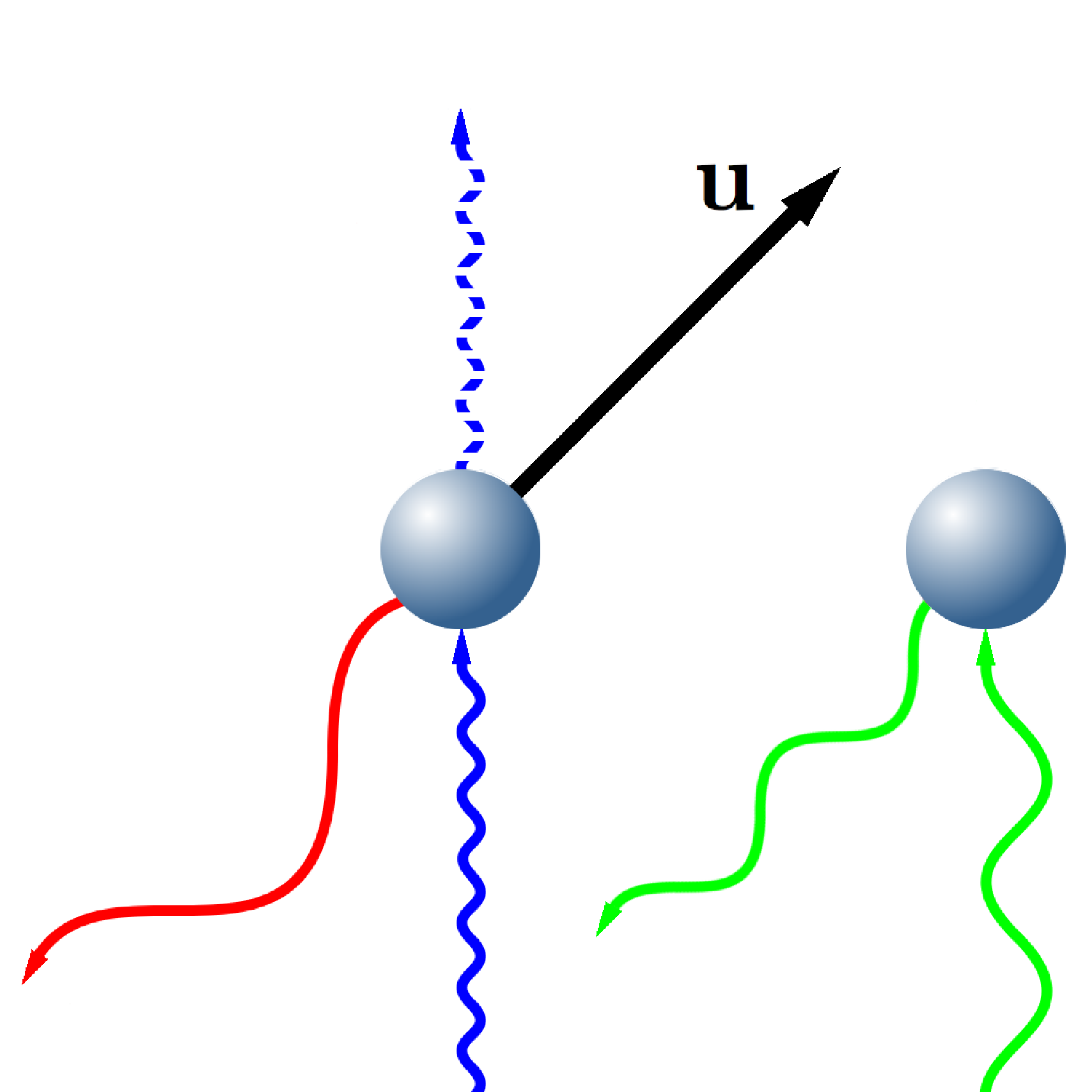
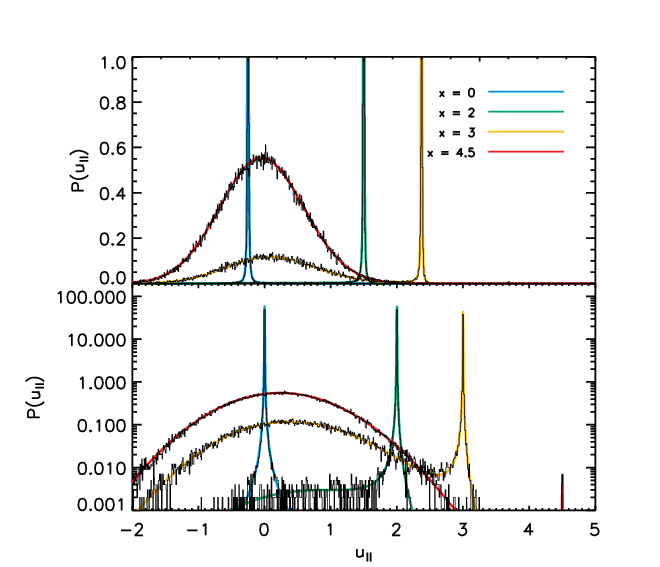
Since the frequency determines the opacity of the gas, the exact value of the velocity is important. In the directions perpendicular to , the velocities will follow a Gaussian distribution . However, due to the resonance nature of the scattering event, the velocity parallel to depends on . Thus, the probability distribution must be convolved with the probability of the atom being able to scatter the photon. For small values of , being scattered by an atom with is highly favored. For large values of the abundance of these atoms decrease as , so that scattering by “slow” atoms becomes more probable, even though in reference frame of these atoms the photon is far in the wing. The resulting normalized probability distribution is
| (13) |
Since Eq. (13) is not analytically integrable, is generated from this distribution by means of the rejection method [56]: a random value of a comparison function that is integrable and lies everywhere above is found, and accepted if a second random number33 3 Random numbers in the interval are generated by means of the subroutine ran1 [56]. (a “univariate”) is less that the ratio of the two functions. Due to the peculiar shape of (see Fig. 2), following Zheng & Miralda-Escudé [89], two comparison functions are used. For the wide range of temperatures and frequencies involved we find that a satisfactory average acceptance-to-rejection ratio of order unity is achieved for
| (14) |
as the value separating the two comparison functions. Here defines the boundary between the core and the wings of the Voigt profile, i.e. where . The solution to this equation can be approximated as
| (15) |
When , the photon barely diffuses spatially. Only when it has diffused sufficiently far in frequency space will it be able to make a large journey in real space. The photon may scatter thousands or even hundreds of thousands of times before entering the wing of the line profile. These scatterings are insignificant in the sense that they do not contribute to any important displacement in neither space nor frequency. Hence, we may as well skip them altogether and go directly to the first scattering that pushes the photon into the wing. This highly efficient acceleration of the code is achieved following Ahn et al. [4]: if is less than some critical value , is drawn from a truncated Gaussian so as to favor fast moving atoms and artificially push the photon back in the wing. The resulting random velocity generator can be written [14] as
| (16) |
where and are two univariates.
However, the value is not simply equal to , since for a nondense medium, a core scattering can in fact be associated with a considerable spatial journey, while for clouds of extremely high density even scatterings in the inner part of the wing may be neglected. Moreover, the exact value of is actually quite important; this acceleration scheme can decrease the computational execution time by several orders of magnitude but too high values will push the photons unnaturally far out in the wings, leading to incorrect results. From the Neufeld solution we know that the important parameter is the product . Correspondingly, we expect to be a function of the value of in the current cell. Indeed, it is found that the value
| (17) |
where or for or , respectively, can be used without affecting the emergent spectrum in both various tests (§IV) and realistic situations (§VI). Of course, if the photon is already in the wing, the proper Gaussian velocity distribution is used, i.e. .
The final frequency of the scattered photon (in the reference frame of the fluid element) depends on direction in which the photon is scattered, given by the phase (probability) function
| (18) |
where is the angle between and the outgoing direction , and is the degree of polarization for scattering. For reasons of symmetry, the scattering must always be isotropic in the azimuthal direction and hence independent of . For scattering in the line center, i.e. for , transitions to the state results in isotropic scattering such that , while the transition causes some polarization, resulting in [28]. Since the spin multiplicity is , with the angular momentum of the state, the probability of being excited to the state is twice as large as being excited to the state44 4 For the environments produced here, transitions to the state and subsequent destruction of the photon through two-photon processes can be neglected.. For scatterings in the wing, polarization for scattering is maximal, i.e. [71].
The transition between the wing and the core is taken to occur at . Obviously, the phase function does not change abruptly at this point, but rather varies continuously from one to another in some fashion. However, the difference in the final outcome is very small, even if a single phase function is used for all scatterings.
In the observers frame, the final frequency is then
| (19) |
where the factor [21], with the Planck constant, accounts for the recoil effect.
After the scattering, the photon is assigned a new, random value of and continues its journey.
III.4. Observations
Following the above scheme, the photon is trailed as it scatters trough real and frequency space, until eventually it escapes the computational box. Subsequently, this procedure is repeated for a number ( in total) of photons sufficiently large that the result converges. Here, “convergence” is defined as the change in the desired result after photons as compared to the result after photons being on the % level. If we merely concern ourselves with the characteristic angularly averaged spectrum of escaping Ly photons, needs not be very large, of the order . However, since in general the morphology of a galaxy may very well cause an anisotropic luminosity, it may be more interesting to see how the system would appear when observed from a given angle, at a distance given by the redshift of the galaxy. Because the ratio of photons escaping in a particular direction is effectively zero, following Yusuf-Sadeh & Morris [86] we calculate instead for each scattering and for each photon the probability of escaping the medium in the direction of the observer, or, in fact, six different observers situated in the positive and negative directions of the three principal axes, as , where is now given by the angle between and the direction of the observer and is the optical depth of the gas lying between the scattering event and the edge of the computational box (integrated through the intervening cells and of course taking into account the different bulk velocities of the cells).
This probability is added as a weight to a three-dimensional array (“CCD”) of two spatial and one spectral dimension. Each pixel suspends a solid angle of the computational box. The total surface brightness SBpix of the area covered by the pixel, measured in energy per unit time, per unit area at the location of the observer, per unit solid angle suspended by the pixel is then
| (20) |
where is the luminosity distance given by the redshift, and the sum is over all photons and all scatterings. Note that Eq. (20) does not contain a factor , due to the fact that the phase functions are normalized to unity.
Eq. (20) is the SB that an observer would measure at a distance from the galaxy. Hence, this is the interesting quantity for comparing with actual observations. Theorists tend to be more concerned with the intrinsic SB, i.e. the flux measured by a hypothetical observer at the location of the source. In this case Eq. (20) must be multiplied by a factor , and the SB is then measured in energy per time per area.
When a sufficient number of photons has been propagated, the 3D array can be collapsed along the frequential direction to give a “bolometric” Ly SB map, along the two spatial directions to give the integrated spectrum, or along all directions to give the total flux received from the source. Since in fact we obtain a full spectrum for each pixel, it is also possible to perform 2D (long slit) spectroscopy, giving frequency as a function of position of a selected part of the image.
For the spectra to converge, should be of order . The luminous regions of the SB maps need to converge, while the outer regions need several . However, when smoothing the maps so as to simulate the effect of the atmosphere, or in any case a finite angular resolution, and averaging the SB maps in the azimuthal direction to produce SB profiles, less photons are needed, of order . In the simulations described in §VI, – was used.
IV. Testing the Code
IV.1. Individual Scatterings
The various probability distribution generators were tested against their analytical solutions (in the case such solutions exist; otherwise against numerical integration). We show here only the result for the parallel velocities (Fig. 2).
To test the individual scatterings, Fig. 3 shows the relation between the frequency of the incident and of the scattered photon, compared with the exact redistribution function as formulated by Hummer [35].
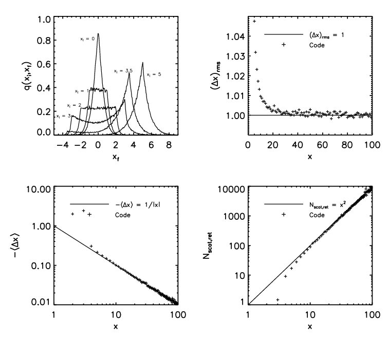
Furthermore, the rms and mean shift, and the average number of scattering before returning to the core for wing photons are shown. For , the values are seen to converge to the results derived by Osterbrock [50], and given by Eqs. (3) and (4).
IV.2. Uniform Slab of Gas
The most basic confirmation of the reliability of the code is a test of the Neufeld solution. Hence, a simulation of a slab (i.e. with the - and -dimension set to infinity) is run in which the bulk velocity of the elements is set to zero, while the temperature and hydrogen density are constant in such a way as to give the desired line center optical depth from the center of the slab to the surface. Base cells are refined in arbitrary locations, to an arbitrary level of refinement. Also, constant is used and the recoil term in Eq. (19) is omitted to match the assumptions made by Neufeld. The result for different values of is shown in Fig. 4, while the result of varying the initial frequency is shown in Fig. 5.
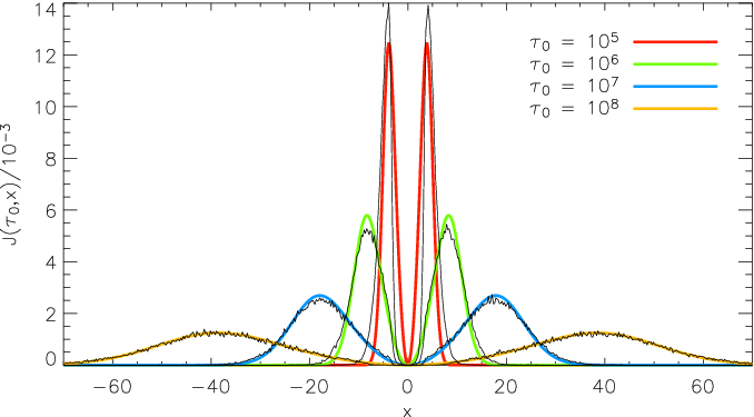
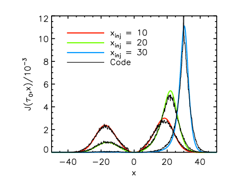
For the lowest optical depth (, corresponding to at K), the fit is not very accurate. However, this is not an artifact caused by, e.g., a too low number of photons in the simulation, but merely reflects the fact that the Neufeld solution is no longer valid when the optical depth becomes too low (at low optical depths, the transfer of photons is no longer dominated by wing scatterings, where the line profile can be approximated by a power law).
Figure 6 shows the average number of scatterings .
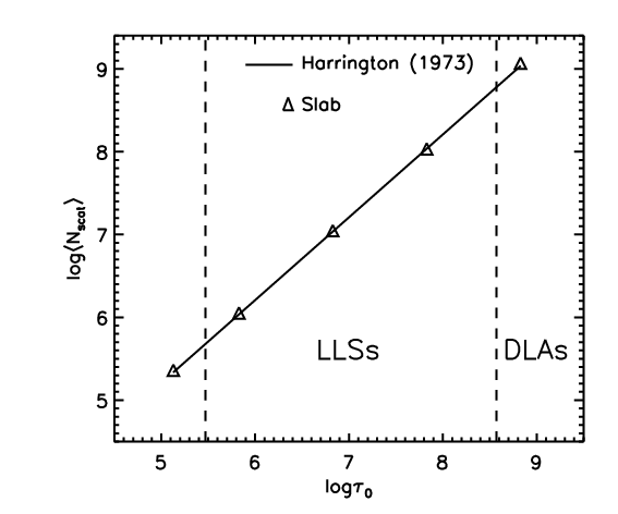
Of course, in this case a non-accelerated version of the code (i.e. ) was used, since we are interested in the true number of scatterings. To get a feeling for the physical significance of the optical depths, the region of is divided into the domains of the so-called Lyman-limit systems (LLSs) and damped Ly systems (DLAs), characterized by limiting neutral hydrogen column densities of cm-2 and cm-2, respectively.
IV.3. Gas Bulk Motion
Except for slightly different factors, Dijkstra et al. [14] found that the emergent spectrum, its maximum, and the average number of scatterings of an isothermal, homogeneous sphere with no bulk velocity of the gas resemble those of the slab. Although not shown here, such simulations were also carried out, and were run in two different ways; with a version of the code that has concentric shells instead of cells, thus exploiting fully the spherical symmetry, and a normal, cell-based version, the output of which converges to the former for sufficiently high resolution.
To test if the implementation of the bulk velocity scheme produces reliable results, we inspect the emergent spectrum of a sphere subjected to isotropic, homologous expansion or collapse. Thus, the velocity of a fluid element at a distance from the center is set to
| (21) |
where the Hubble-like parameter is fixed such that the velocity increases linearly from 0 in the center to a maximal absolute velocity at the edge of the sphere ():
| (22) |
with positive (negative) for an expanding (collapsing) sphere.
For K, no analytical solution for the spectrum exists. Qualitatively, we expect an expansion to cause a suppression of the blue wing and an enhancement of the red wing of the spectrum. The reason for this is that photons blueward of the line center that would otherwise escape the medium, are shifted into resonance in the reference frame of atom lying closer to the edge, while red photons escape even more easily. Conversely, a collapsing sphere will exhibit an enhanced blue wing and a suppressed red wing. This is indeed seen in Fig. 7.
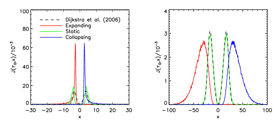
Another way to interpret this effect is that photons escaping an expanding cloud are, on the average, doing work on the gas, thus losing energy, and vice versa for a collapsing cloud.
In Fig. 8, results for a sphere of gas expanding at different velocities are shown.
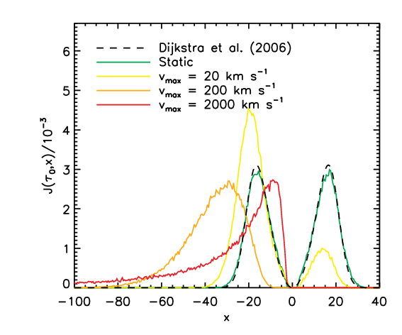
For increasing , the position of the red peak is progressively enhanced and displaced redward of the line center. However, above a certain threshold value the velocity gradient becomes so large as to render the medium optically thin and allow less redshifted photons to escape, making the peak move back toward the line center again.
V. Semianalytical Acceleration Scheme
Most of the computing time is spent in the very dense cells. Since each cell is in fact a “uniform” cube, i.e. a cube of homogeneous and isothermal gas, if an analytical Neufeld-equivalent solution for the distribution of frequency exists, it would be possible to skip a great number of scatterings and thus speed up the code further.
The slab solution is an alternate series which can be written in closed form. Unfortunately, this is not feasible for the cube solution, but under certain approximations, Tasitsiomi [77] found that it is still possible to write it as an alternate series. The problem is that, whereas for the slab the terms quickly die off, the same is not true for the cube. In fact she found that to achieve an accuracy better than 3%, one must exceed 30 terms.
Hence, it seems more convenient to seek a “Neufeld-based” approximation. Since for the cube, the radiation can escape from six faces rather than just two, we may expect the emergent radiation to be described by a function similar to the slab solution, but using a lower value of .
V.1. Emergent Spectrum
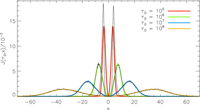
Toward these ends, a series of simulations is run in which photons are emitted isotropically from the center of a cube of constant — but different — temperature and density, and zero bulk velocity. The distance from the center to each face is . We will investigate optical depths , , , and (measured along the shortest path from center to face). In all simulations, , and different temperatures are tested. We then fit a Neufeld profile to the emergent spectrum, using as the independent variable, where is the parameter to be determined. A priori, we have no reason to believe that the same value of , if any, should be able to describe all optical depths. However, it is found that, save for the lowest optical depth (), excellent fits are obtained using
| (23) |
This is seen in Fig. 9.
V.2. Directionality of the Emergent Photons
In realistic, cosmological simulations, the direction with which the photons exit the cell is also important. Since in the limit , any finite size step not perpendicular to the surface will just shift to position of the photons in the parallel direction, for extremely optically thick slabs, the photons should have a tendency to exit perpendicular to the surface. In this case, Phillips & Mészáros [54] found that the directionality of the emergent radiation approaches that of Thomson scattered radiation from electrons, with intensity
| (24) |
where , with the angle between the outgoing direction of the photon and the normal to the surface.
Since the number of photons emerging at is , the probability of exiting the slab with is [77]
| (25) | |||||
We confirm that this is also an excellent description for a cube (Fig. 10).
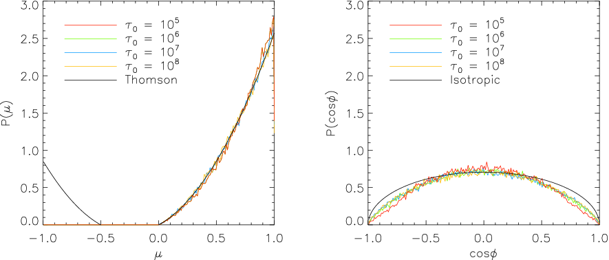
The probability distribution is found by differentiating Eq. (25) and recognizing that must be positive for the photon to escape:
| (26) |
Since Eq. (26) is valid for all six faces of the cube, the azimuthal angle parallel to the face cannot, as in the case of a slab, be evenly distributed in [77]. However, as can be seen from Fig. 10, the deviation from uniformity is quite small, and can probably be neglected. Furthermore, it seems less pronounced, the higher the optical depth.
V.3. Point of Escape
The final parameter characterizing the photons escaping the cube is the point where it crosses the face. Figure 11 shows the azimuthally averaged SB profiles of the emergent radiation as a function of distance from the center of the face, for different optical depths.
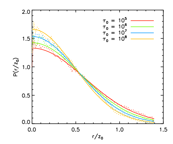
It is found that the SB profile is fairly well described by a truncated Gaussian
| (27) |
The dispersion of the SB decreases very slowly with
optical depth, and can be written as
.
However, in the context of a cell-based structure, one might state that it is
meaningless to discuss differences in position on scales smaller than the size
of a cell, and it is found that final results are not altered by simply setting
.
V.4. Implementation of the Cube Solution
With the probability distributions of frequency, direction and position for the photons escaping the cell, we are now able to accelerate the code further: every time a photon finds itself in a host cell of higher than some given threshold, which to be conservative we define as , an effective cell with the photon in the center is built, with “radius” equal to the distance from the photon to the nearest face of the host cell. Since the effective cell is always completely circumscribed by the host cell, its physical parameters are equal to those of its host cell.
If the value of in the effective cell, , is below the threshold (i.e. if the photon is too close to the face of the host cell), the normal scheme is used. Otherwise, the photon is assigned a new frequency according to the effective Neufeld distribution: drawing a univariate and setting this equal to the Neufeld-equivalent cube solution55 5 Of course normalized to unity instead of the usual integrated from to yields (after some algebra)
| (28) | |||||
Inverting the above expression, the frequency of the photon then becomes
| (29) |
VI. Application to Cosmological Simulations
To demonstrate the potency of the developed code, we apply it to a number of different simulated galaxies. Specifically, we will study three young “Lyman-break galaxies” (LBGs), for the purpose of the present study dubbed K15, K33, and S115, at a redshift of , at which time the Universe was Gyr old. These three galaxies are representative of typical galaxies in the sense that the two larger evolve into Milky Way/M31-like disk galaxies at , whereas S115 becomes a somewhat smaller disk galaxy. The characteristic circular velocities of the galaxies at are 245, 180 og 125 km s-1, respectively.
The cosmological simulation is conducted using an N-body/hydrodynamical
TreeSPH code. A “pseudo”-RT scheme of the ionizing UV
radiation is accomplished on-the-fly, while a more comprehensive
UV RT scheme is implemented post-process. This is described below.
VI.1. Underlying Cosmological Simulations
The numerical simulations are first carried out at low resolution, but in a large volume of space. Subsequently, interesting galaxy forming regions are resimulated at high resolution. Typically, resimulations are performed at 64 higher mass resolution. In order to check the significance of the resolution, also lower resolution (8) and ultrahigh resolution (512) simulations are executed.
The simulations are started at an initial redshift , at which time there is only dark matter (DM) and gas SPH particles. The latter eventually evolves partly into star particles, while, in turn, star particles can become gas particles again. The star formation criteria is described in Sommer-Larsen et al. [67]. For K15 and K33, a Kroupa [40] initial mass function (IMF) has been assumed, while for S115, a Salpeter [63] IMF was used. A standard CDM is assumed, i.e. , , and the rms linear density fluctuation on scales of Mpc is . In addition to hydrogen and helium, the code also follows the chemical evolution of C, N, O, Mg, Si, S, Ca, and Fe, using the method of Lia et al. [43].
Additional information about the simulations can be found in Tab. 1, while Tab. 2 summarizes the physical properties of the resulting galaxies, demonstrating that they are typical of galaxies at –5. Having an -band magnitude of , K15 and K33 could be detected as LBGs in a survey like the one of Steidel et al. [69, = R lim 25.5 ]. With , S115 is too faint to be detected as an LBG in current surveys, although the limit is being approached [e.g. 64, reaching ].
| Galaxy | K15 | K33 | S115 | |||||
|---|---|---|---|---|---|---|---|---|
| Resolution | 8 | 64 | 8 | 64 | 64 | 512 | ||
| , | ||||||||
| , | 382 | 191 | 382 | 191 | 191 | 96 | ||
| 680 | 340 | 680 | 340 | 340 | 170 | |||
| 20 | 10 | 20 | 10 | 10 | 5 | |||
Note. — Total number of particles, number of SPH particles only, masses , gravity softening lengths , and minimum smoothing lengths of dark matter (DM), gas (SPH), and star particles used in the simulation of the three galaxies K15, K33, and S115, for different resolutions. Masses are measured in , distances in pc.
| Galaxy | K15 | K33 | S115 |
|---|---|---|---|
| SFR/ yr-1 | 16 | 13 | 0.5 |
| /km s-1 | 245 | 180 | 125 |
| /kpc | 47.5 | 37.3 | 22.0 |
| /erg s-1 | |||
| /erg s-1 Hz-1 |
Note. — Star formation rates (SFRs), stellar masses () circular velocites (), virial radii (), Ly luminosities (), and UV luminosities () for the three simulated galaxies K15, K33, and S115. All quoted values correspond to a redshift of , except which is given for .
The Ly emission is produced by three different processes [41, see also], viz. from recombinations in photoionized regions around massive stars (responsible for % of the total Ly luminosity), gravitational cooling (%), and a metagalactic UV background (UVB) photoionizing the external parts of the galaxy (%). In the first case, the luminosity is determined following Fardal et al. [18], using the code Starburst99 [42] to yield the Lyman continuum (LyC), and assuming a mean LyC photon energy of 1.4 Rydberg and that 0.68 Ly photons are emitted per photonionization. The gravitational cooling is accounted for by keeping track of temperature and ionization state of the gas. The UVB field is assumed to be that given by Haardt & Madau [27], where the gas is treated as optically thin to the UV radiation until the mean free path of a UV photon at the Lyman limit becomes less than 1 kpc, at which point the gas is treated as optically thick and the UV field is “switched off”.
For a more thorough description of the code, the reader is referred to Sommer-Larsen et al. [67], and to Sommer-Larsen [66] for recent updates.
VI.2. Ionizing UV Radiative Transfer
To model the propagation of ionization fronts realistically, Razoumov & Sommer-Larsen [58], Razoumov & Sommer-Larsen [59] implemented the following RT scheme as a post-process to the cosmological simulation: the position of the SPH particles and their associated physical properties are interpolated from the 50 nearest neighboring particles onto a grid of base resolution cells. Dense cells are subdivided in eight cells, which are further refined until no cell contains more than ten particles.
Around each stellar source, a system of radial rays is built that split either as one moves farther away from the source or as a refined cell is entered, and is the angular resolution level. Once a radial ray is refined angularly, it stays refined at larger distances from the source, even when leaving the high-resolution region. In each cell, the photoreaction number and energy rates due to photons traveling along ray segments passing through that cell are accumulated. These rates are then used to update temperature and the ionization state of hydrogen and helium, which in turn are used to calculate the LyC opacities used in the RT. In addition to stellar photons, we also account for ionization and heating by LyC photons originating outside the computational volume with the FTTE scheme [57] assuming the Haardt-Madau UVB.
Although the UV RT is not coupled to hydrodynamics, hydrodynamical (shock) heating needs to be taken into account during the RT. All cells with temperatures above in the SPH output are considered to be shock-heated, and during the RT only their ionization state, not their temperature, is updated. For all cells with temperatures below a hydro-heating term is computed, which is defined as the amount of heating needed to keep the temperature of that cell constant if its ionization state stayed at the original level. This hydro-heating term is used to update both temperature and ionization of all cells. For these cells, a temperature ceiling of is used to avoid unphysical overheating, as during the RT calculation heated gas is not allowed to expand.
VI.3. Ly Radiative Transfer
For the purpose of the Ly RT, the same AMR grid is used as for the UV RT. A (250 kpc)3 box is cut out from each snapshot and is refined to or 8 levels, where corresponds to the unrefined (base) grid. Thus, the cell size of the smallest cells is merely pc, more than four orders of magnitude smaller than the computational box itself and comparable to the size of molecular clouds.
VI.3.1 Significance of the Improved UV RT
Initially, we will focus on K15, consisting of two rather compact “disks” embedded in a more extended, –15 kpc thick, sheet-like structure composed of nonstar-forming H i gas, taken to constitute the -plane. Figure 12 shows the general effect of the scattering: the SB is increased in the outskirts of the galaxy, at the expense of a decrease in the center, where most of the photons are produced. The effect on the spectrum is also seen: while the only broadening of the input spectrum visible is due to the bulk motion of the gas elements emitting the photons (the natural broadening being much smaller), the scattered spectrum is severely broadened, diminished by more than an order of magnitude, and split up into two peaks due to the high opacity of the gas for photons in the line center.
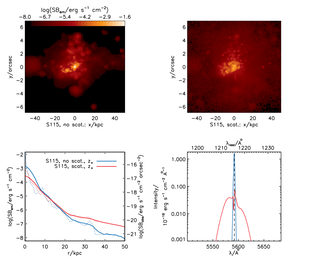
Figure 13 shows the emergent spectrum, as observed when viewing the sheet edge-on and face-on, respectively. For each case, four spectra are shown: i) using the temperature and ionization from the original SPH run, ii) using the temperature and ionization computed with the LyC transfer scheme from Sec. VI.2 applied to stellar photons only, iii) using the temperature and ionization from a model in which the UVB is traced with the FTTE scheme and there are no stellar photons, and iv) using distributions from a model in which LyC RT is computed for both stellar and UVB photons.
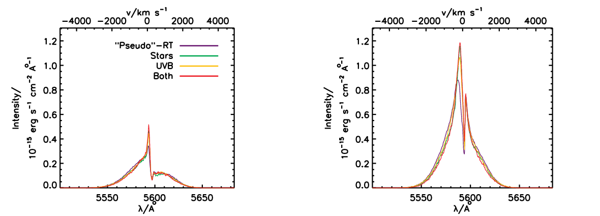
As expected, fewer photons escape in the plane of the sheet, as the Ly optical depth in this direction is greater and more photons scatter and eventually escape in the directions perpendicular to the sheet. Note that both edge-on and face-on spectra are sensitive to the changes in ionization of predominantly low-density regions which is computed with LyC radiative transfer. As discussed in §II.2, the quantity that determines the shape of the spectrum is the product (at a fixed physical size). Generally, a higher temperature will also imply a lower density of neutral hydrogen, and vice versa, and thus we might expect to change rapidly to higher or lower values for the improved scheme. However, for high density cells the change in the ratio is minor when invoking the improved scheme, in most cases of order unity. Only in low density cells is this ratio considerably altered, but since % of all scatterings take place in high-density cells, the overall effect is small. The only notable difference is seen in the inner part of the spectrum, which is exactly the part that is created by the low-density regions, since photons near the line center cannot escape from high-density regions.
VI.3.2 Characteristics of the Emergent Spectrum
The double peak profile seen in Fig. 13 is characteristic of Ly emission lines; the high opacity for photons near the line center makes diffusion to the either side necessary in order to escape the galaxy. Nonetheless, unlike in previous simple models, the intensity in the line center is not zero. The photons that contribute to this intensity are those produced mainly by gravitational cooling, in the outskirts of the systems.
Figures 14 and 15 display the spectra emerging from galaxies K33 and S115 at , in six different directions.
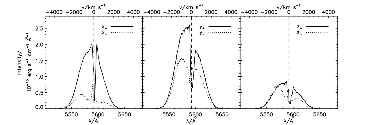
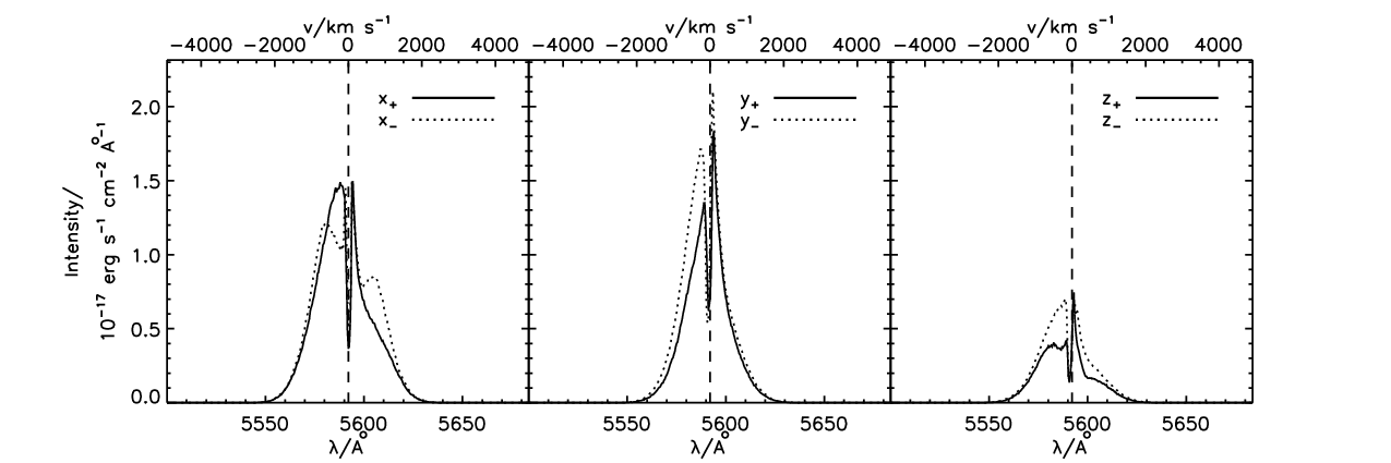
The exact shape varies quite a lot, but all spectra appear to exhibit the double peak profile. Moreover, they are broadened by several 1000 km s-1.
Double peaks have been observed on several occasions [85, 82, e.g.,]. Tapken et al. [75], using a resolution of , found three out of 16 LAEs at redshifts – to have a double-peaked profile, while Yamada et al. (priv. comm.), using found that 26 of 94 LAEs at redshift 3.1 have the double-peaked profile. The difference in magnitude of the two peaks can be a signature of infalling/outflowing gas, cf. §IV.3. In principle, this difference may be used as a probe of the gas dynamics, and has indeed been used to infer the presence of galactic superwinds. However, since LAEs are often situated in higher-than-average density regions, the removal or diminishing of the blue peak might also be caused by IGM resonant scattering combined with cosmic expansion.
Even if the double peak survives intergalactic transmission, fairly high resolution is required. With a typical separation of the peaks of the simulated spectra from a few to Å, the resolution must be –.
It is interesting that while the Ly profile of the sub-Milky Way galaxy K15 also shows a moderate gas infall, we see some outflow signatures in the spectrum of the lower-mass galaxy S115 from negative - and -directions. Fitting a Neufeld, or Dijkstra, profile to the observed spectra can give us an idea of the intrinsic properties of the system. Unfortunately, due to the degeneracy between column density and temperature, one would have to gain knowledge either of the parameters by other means to constrain the other (e.g. by inferring column density from the spectrum of a coincident background quasar, or by assuming a temperature of, say, K, representative of most of the Ly emitting gas). However, clumpiness of the ISM will lower the effective optical depth, making any inferred value of a lower bound. This is exactly the reason we need realistic models; galaxies are not isothermal, homogeneous slabs.
VI.3.3 Surface Brightness
Figure 16 displays the Ly SB maps, integrated over the line, of two of the galaxies, K15 and K33.
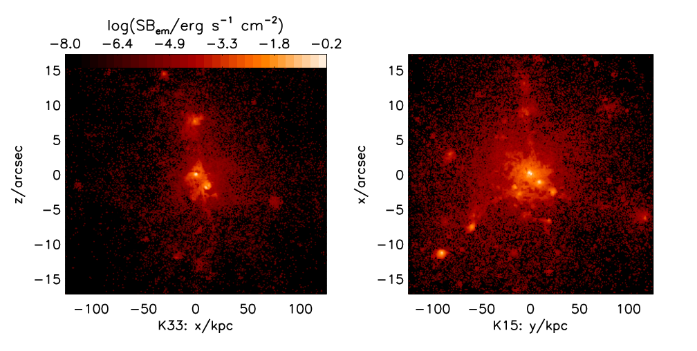
As mentioned already, K15 is embedded in a sheet-like structure, lying at the intersection of three filaments of gas. Since the bulk of the photons are produced in the central, star-forming regions, the total optical depth is larger in the direction parallel to the sheet than perpendicular to it, and hence we would expect the photons to escape more easily in the face-on direction. Similarly, K33 is situated in a filament of gas, taken to lie along the -axis. Here, we would expect the photons to escape more easily in the - and -directions.
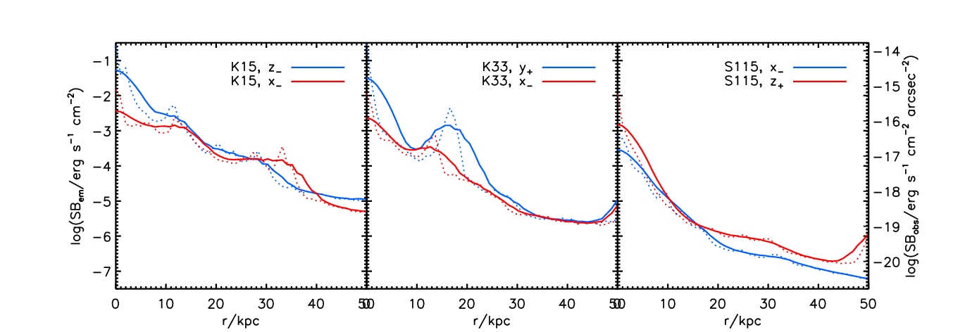
Averaging the SB in the azimuthal direction, the SB profiles of the three galaxies, each as viewed from two different directions, are shown in Fig. 17, while Tab. 3 summarizes the observed maximum surface brightnesses, SBmax.
| Galaxy | K15 | K33 | S115 |
|---|---|---|---|
| log SB | |||
| log SB | |||
| log SB | |||
| log SB | |||
| log SB | |||
| log SB | |||
| Ratio | 14.3 | 13.6 | 5.3 |
Note. — Surface brightnesses (SBs, calculated from the images convolved with a seeing of ) are measured in erg s-1 cm-2, at the location of the galaxies. The maximally and the minimally observed SBmax’s for a given galaxy are written in boldface, and the ratios between these are given in the lower row.
In fact, regarding K33, SB turns out to be smaller than both SB and SB, due to the presence in the line of sight of hydrogen clouds with little star formation causing a shadowing effect. As seen in Tab. 3, the observed SB of a given galaxy varies with viewing angle by approximately an order of magnitude.
This result is intriguing in relation to the classification of galaxies. Galaxies are commonly annotated according to the method by which they are selected, and one of the mysteries in the context of galaxy formation and evolution is the connection between the different types.
As already mentioned, sufficiently high column densities of neutral hydrogen in the line of sight toward a bright background source give rise to broad absorption lines in their spectra, and may be detected as the so-called DLAs. On the other hand, galaxies with high enough star formation rates (SFRs) may be detected in narrowband searches by an excess of their narrowband to continuum flux as LAEs.
Due to the massive amount of neutral hydrogen, DLAs are self-shielded against ionizing radiation and may hence be able to cool sufficiently to initiate star formation. The assumption that DLAs be progenitors of present-day galaxies therefore seems reasonable, and is indeed generally accepted. Pursuing this idea, one may thus image an evolutionary sequence, for instance DLA LAE LBG [23, 25, see, e.g.,]. However, high-redshift galaxy classification may also be a simple consequence of a selection effect, i.e. reflecting the means by which they are probed. It seems safe to say that the exact relation between the different types remains unclear.
All three galaxies of the present study contain enough neutral hydrogen to make them detectable as DLAs in the spectra of (hypothetical) quasars [17, see]. More interestingly, the present results show that while their high SFRs (K15: 16 yr-1; K33: 13 yr-1; S115: 1/2 yr-1) may make at least the two larger galaxies detectable as LAEs when viewed from a given direction, it may not be possible to see them in Ly from another direction; instead, it may be possible to observe them as LBGs. This effect demonstrates how galaxies selected by different means may be connected to each other, although this obviously has to be quantified through detailed modeling, including the effect of dust.
Overlaps in the properties of LAEs and LBGs have also been inferred observationally; Gawiser et al. [24] found that more than % of a sample of emission-line-selected LAEs have the right -colors to be selected as LBGs. The primary difference between the two populations is the selection criteria, as only % are also brighter than the “spectroscopic” LBG magnitude cut. Also, when correcting for dust, Gronwall et al. [26] found comparable SFRs for the two populations.
For high-redshift LAEs, SFRs are inferred almost exclusively from Ly flux measurements, assuming isotropic luminosity. However, as is evident from the above discussion, in general the complex morphology of a galaxy may very well cause a preferred direction of photon escape. For the three galaxies of the present study, the angular variation in flux can be as high as a factor of 3.4, 6.2, and 3.3, for K15, K33, and S115, respectively (here the flux is calculated by integrating the SB maps over a region of radius kpc, centered at ). Although not as pronounced as in the case of SBmax, this introduces a considerable source of uncertainty, which may propagate into estimates of SFRs or into calculations of the content of dust residing in galaxies.
VI.3.4 Testing Resolution and Interpolation Scheme
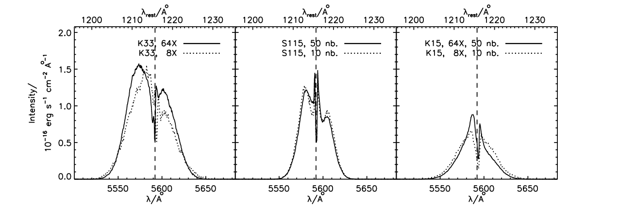
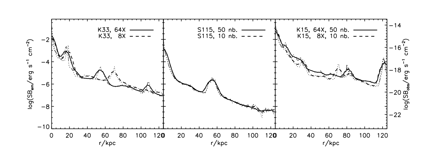
In order to check the impact of the resolution of the cosmological simulation on the results of the Ly RT, the above RT calculations were also carried out on the output of cosmological simulations performed at eight times lower resolution. Furthermore, the procedure by which the SPH particles were interpolated onto the grid was tested by using the 10 nearest neighboring particles instead of the usual 50 particles, and running similar RT calculations on the output grids. Although in both cases the results changed somewhat, there seems to be no general trend. Due to the slightly different evolution of the lo-res galaxies, the precise configuration of stars and gas clouds will not necessarily be the same, and thus luminous peaks in the SB maps cannot be expected to coincide exactly. However, the maximum SBs appear to agree to within a few tens of percents, as do the slopes and the overall amplitudes of the SB profiles. The outcome of three such simulations can be
VII. Summary and Discussion
A Monte Carlo Ly radiative transfer code has been presented, and subsequently tested against various analytical solutions. The code is capable of propagating Ly radiation on an adaptively refined mesh, with an arbitrary distribution of Ly source emission, gas temperature, density, and velocity field, and is thus suitable for making predictions about the diffusion of Ly radiation in simulated galaxies of arbitrarily high resolution.
A similar non-AMR version of the code has already verified the extendedness of Ly surface brightness of –4 compared to the continuum as being due to the resonant scattering of Ly [41]. In the present work, we address the question of the impact of the viewing angle on the observed properties of galaxies. We find that the anisotropic escape of photons may cause the maximum observed SB to vary quite a lot — in the three studied cases on the average by approximately an order of magnitude — while the total observed Ly flux varies somewhat less; a factor of 3–6. We propose that this effect may sometimes cause confusion in the classification of galaxies, in the sense that the same galaxy could be detected as an LBG from one direction and a LAE from another. In addition, this angular variation may act as a source of error when inferring star formation rates.
As yet, the developed code includes no effect of dust. Considerable amounts of dust have been inferred to reside in LBGs [65, 10, 72, 62, e.g.,]. Correcting for dust increases the typical inferred value of the SFR by a factor of [60]. One may naively expect the presence of dust to amplify the difference between the SB observed from different angles of inclination. Nevertheless, taking Ly transfer into account, it is not obvious how observations will be affected by dust. In fact, the Ly-to-continuum ratio may even be boosted if most of the dust resides in clump together with the neutral gas, since Ly will scatter off the clouds while continuum photons get absorbed [49, 29]. Also, since the presence of dust induces the formation of hydrogen molecules, it may actually lower somewhat, making it easier for the photons to escape.
The transfer of the Ly photons through the intergalactic medium has not been modeled either. IGM absorption may remove the blue peak of the spectrum, since the cosmological expansion will eventually shift it into resonance of neutral hydrogen in the line of sight, thus approximately halving the observed flux. The damping wing of the absorption profile may sometimes extend into the red wing, attenuating the line even more. On the other hand, the effect of IGM may be substantially reduced, since the line-of-sight density of Hi absorbers decrease with decreasing redshift, and by , the Universe is largely ionized. The implementation of dust and IGM RT will presented in a forthcoming paper.
References
- [1] Adams, T. F. 1972, ApJ, 174, 439
- [2] Ahn, S.-H., Lee, H.-W., & Lee, H. M. 2000, JKAS, 33, 29
- [3] Ahn, S.-H., Lee, H.-W., & Lee, H. M. 2001, ApJ, 554, 604
- [4] Ahn, S.-H., Lee, H.-W., & Lee, H. M. 2002, ApJ, 567, 922
- [5] Ambarzumian, V. A. 1932, MNRAS, 93, 50
- [6] Auer, L. H. 1965, ApJ, 153, 783
- [7] Avery, L. W. & House, L. L. 1968, ApJ, 152, 493
- [8] Bonilha, J. R. M., Ferch, R., Salpeter, E. E., Slater, G., & Noerdlinger, P. D. 1979, ApJ, 233, 649
- [9] Bouwens, R. J. et al. 2004, ApJ, 616, 79
- [10] Calzetti, D. 2001, PASP, 113, 1449
- [11] Cantalupo, S., Porciani, C., Lilly, S. J., & Miniati, F. 2005, ApJ, 628, 61
- [12] Caroff, L. J., Noerdlinger, P. D., & Scargle, J. D. 1972, ApJ, 176, 439
- [13] Chandrasekhar, S. 1935, ZAp, 9, 267
- [14] Dijkstra, M., Haiman, Z., & Spaans, M. 2006, ApJ, 649, 14
- [15] Djorgovski, S. & Thompson, D. J. 1992, IAUS, 149, 337
- [16] Dunlop, J. S., Le Fevre, O., Franx, M., & Fynbo, J. P. U 2007, Principal Investigators of the Ultra-VISTA project
- [17] Ellison, S. L., Hennawi, J. F., Martin, C. L., & Sommer-Larsen, J. 2007 MNRAS, 378, 801
- [18] Fardal, M. A., Katz, N., Gardner, J. P., Hernquist, L., Weinberg, D. H., & Davé, R. 2001, ApJ, 562, 605
- [19] Feautrier, P. 1964, CR, 258, 3189
- [20] Ferland, G. J. et al. 1998, PASP, 110, 761
- [21] Field, G. 1959, ApJ, 129, 551
- [22] Gardner, J. P. 2006, Astronomical Facilities of the Next Decade, 26th meeting of the IAU
- [23] Gawiser, E. 2006, ASP Conf. Ser., 352, 177
- [24] Gawiser, E. et al. 2006, ApJ642, L13
- [25] Gawiser, E. et al. 2007, ApJ, 671, 278
- [26] Gronwall, C. et al. 2007, ApJ, 667, 79
- [27] Haardt, F. & Madau, P. 1996, ApJ, 461, 20
- [28] Hamilton, D. R. 1940, Phys. Rev, 58, 122
- [29] Hansen, M. & Oh, S. P. 2006, MNRAS, 367, 979
- [30] Harrington, J. P. 1973, MNRAS, 162, 43
- [31] Hartmann, L. W., Huchra, J. P., Geller, M. J., O’Brien, P., & Wilson, R. 1988, ApJ, 326, 101
- [32] Henyey, L. G. 1940, PNAS, 26, 50
- [33] Hu, E.M., Cowie, L. L., & McMahon, R. G. 1998, ApJ, 502, 99
- [34] Hu, E.M., Cowie, L. L., Capak, P., McMahon, R. G., Hayashino, T., & Komiyama, Y. 2004, AJ, 127, 563
- [35] Hummer, D. G. 1962, MNRAS, 125, 21
- [36] Iye, M., Ota, K., & Kashikawa, N. 2006, BAAS, 38, 1079
- [37] Jefferies, J. T. & White, O. R. 1960, ApJ, 132, 767
- [38] Koelbloed, D. 1956, BAN, 12, 341
- [39] Kollmeier, J. 2006, Ph.D. thesis: The Intergalactic Medium: Absorption, Emission, Disruption
- [40] Kroupa, P. 1998, MNRAS, 298, 231
- [41] Laursen, P. & Sommer-Larsen, J. 2007, ApJ, 657, 69
- [42] Leitherer, C. et al. 1999, ApJ, 123, 3
- [43] Lia, C., Portinari, L., & Carraro, G. 2002, MNRAS, 330, 821
- [44] Loeb, R. & Rybicki, G. B. 1999, ApJ, 524, 527
- [45] Meier, D. L. & Terlevich, R. 1981, ApJ, 246, 109
- [46] Miller, G. E., Scalo, J. M. 1979, ApJ, 41, 513
- [47] Natta, A. & Beckwith, S. 1986, A&A, 158, 310
- [48] Neufeld, D. 1990, ApJ, 350, 216
- [49] Neufeld, D. 1991, ApJ, 370, L85
- [50] Osterbrock, D. E. 1962, ApJ, 135, 195
- [51] Ouchi, M. et al. 2003, ApJ, 582, 60
- [52] Panangia, N. & Ranieri, M. 1973, A&A, 24, 219
- [53] Partridge, R. B. & Peebles, P. J. E. 1967, ApJ, 147, 868
- [54] Phillips, K. C. & Mészáros, P. 1986, ApJ, 310, 284
- [55] Pierleoni, M., Maselli, A., & Ciardi, B. 2007, (arXiv:0712.1159)
- [56] Press, W. H., Teukolsky, S. A., Vetterling. W. T., & Flannery, B. P. 1992, Numerical Recipes in FORTRAN — The Art of Scientific Computing, 2nd ed., New York: Cambridge University Press
- [57] Razoumov, A. O. & Cardall, C. Y. 2005, MNRAS, 362, 1413
- [58] Razoumov, A. O. & Sommer-Larsen, J. 2006, ApJ, , 651, 81
- [59] Razoumov, A. O. & Sommer-Larsen, J. 2007, ApJ, , 668, 674
- [60] Reddy, N. A. & Steidel, Charles C. 2004, ApJ, 603, 13
- [61] Rhoads, J. E., Malhotra, S., Dey, A., Stern, D., Spinrad, H., & Jannuzi, B. T. 2000, ApJ, 545, 85
- [62] Rigopoulou, D. et al 2006, ApJ, 648, 81
- [63] Salpeter, E. 1955, ApJ, 121, 161
- [64] Sawicki, M. & Thompson, D. 2005, ApJ635, 100
- [65] Sawicki, M & Yee, H. K. C 1998, AJ, 115, 1329
- [66] Sommer-Larsen, J. 2006, ApJ, 644, L1
- [67] Sommer-Larsen, J., Götz, M., & Portinari, L. 2003, ApJ, 596, 47
- [68] Spitzer, L. 1944, ApJ, 99, 1
- [69] Steidel, C. C., Adelberger, K. L., Shapley, A. E., Pettini, M., Dickinson, M., & Giavalisco, M. 2003, ApJ, 592, 728S
- [70] Stenflo, J. O. 1976, A&A, 46, 61
- [71] Stenflo, J. O. 1980, A&A, 84, 68
- [72] Takeuchi, T. T. & Ishii, T. T. 2004, A&A, 426, 425
- [73] Taniguchi, Y. et al. 2005, PASJ, 57, 165
- [74] Tapken, C., Appenzeller, I., Mehlert, D., Noll, S., & Richling, S. 2004, A&A, 416, 1L
- [75] Tapken, C., Appenzeller, I., Noll, S., Richling, S., Heidt, J., Meinköhn, E., Mehlert, D. 2007, A&A, 467, 63
- [76] Tasitsiomi, A. 2006a, ApJ, 645, 792
- [77] Tasitsiomi, A. 2006b, ApJ, 648, 762
- [78] Unno, W. 1952a, PASJ, 3, 158
- [79] Unno, W. 1952b, PASJ, 4, 100
- [80] Unno, W. 1955, PASJ, 7, 81
- [81] Valls-Gabaud, D. 1993, ApJ, 419, 7
- [82] Venemans, B.et al. 2005, A&A, 431, 793
- [83] Verhamme, A., Schaerer, D., & Maselli, A. 2006, A&A, 460, 397
- [84] Verhamme, A., Schaerer, D., Atek, H., Tapken, C. 2007, ASPC, 380, 97
- [85] Yee, H. K. C. & De Robertis, M. M. 1991, ApJ, 381, 386
- [86] Yusuf-Sadeh, F. & Morris, M. 1984, ApJ, 278, 186
- [87] Zanstra, H. 1949, BAN, 11, 401
- [88] Zanstra, H. 1951, BAN, 11, 359
- [89] Zheng, Z. & Miralda-Escudé, J. 2002, ApJ, 578, 33