A new calculation for $D(e,e^{\prime}p)n$ at GeV energies

Preprint: JLAB-THY-08-822 Notice: Authored by Jefferson Science Associates, LLC under U.S. DOE Contract No. DE-AC05-06OR23177. The U.S. Government retains a non-exclusive, paid-up, irrevocable, world-wide license to publish or reproduce this manuscript for U.S. Government purposes

Sabine Jeschonnek⁽¹⁾ and J. W. Van Orden^(2,3) Affiliation: (1) The Ohio State University, Physics Department, Lima, OH 45804
(2) Department of Physics, Old Dominion University, Norfolk, VA 23529
and
(3) Jefferson Lab, 12000 Jefferson Avenue, Newport News, VA 23606

August 24, 2026

Abstract

We perform a fully relativistic calculation of the $D(e,e^{\prime}p)n$ reaction in the impulse approximation. We employ the Gross equation to describe the deuteron ground state, and we use the SAID parametrization of the full NN scattering amplitude to describe the final state interactions (FSIs). We include both on-shell and positive-energy off-shell contributions in our FSI calculation. We show results for momentum distributions and angular distributions of the differential cross section, as well as for various asymmetries. We identify kinematic regions where various parts of the final state interactions are relevant, and discuss the theoretical uncertainties connected with calculations at high missing momenta.

pacs

25.30.Fj, 21.45.Bc, 24.10.Jv

I Introduction

Exclusive electron scattering from the deuteron target is very interesting by itself, and also as a very relevant stepping stone towards understanding exclusive electron scattering from heavier nuclei. The $D(e,e^{\prime}p)n$ reaction at GeV energies allows us - and requires us - to carefully study the reaction mechanism. It is necessary to consider final state interactions (FSIs) between the two nucleons in the final state, two-body currents, and isobar contributions. Of these, the FSIs can be expected to be the most relevant part of the reaction mechanisms at the GeV energy and momentum transfers relevant to the study of the transition from hadronic to quark-gluon degrees of freedom. For some recent reviews on this exciting topic, see e.g. [1, 2, 3].

Even though the deuteron is the simplest nucleus, and it has been the subject of considerable attention for a long time, there are several open questions: Is it possible to experimentally determine the high-momentum components of the deuteron wave function even though the nuclear wave function or the momentum distribution are not observables? Will conventional nuclear physics break down or become too cumbersome at some point, and will a description involving quarks become necessary? Are there any six-quark admixtures in the deuteron wave function, and do they have an unambiguous experimental signal? What influence does short range physics have on conventional wave functions, and how can this influence be removed to find an effective potential $V_{low\,k}$ , provided one is interested in low energy scenarios only [4, 5]? Relativistic wave functions are available [6] for the deuteron. And while the calculational effort is still considerable, it can be managed without resorting to super computers. The interest and importance of the $D(e,e^{\prime}p)n$ process is reflected in the fact that recently, a deuteron benchmarking project has been started to investigate the differences between various calculations that are based on non-relativistic wave functions [7].

Anything that we learn about the reaction mechanism of the $D(e,e^{\prime}p)n$ reaction has implications for heavier targets or experiments where the deuteron is used as a lab. Some examples for the latter are the measurement of the neutron magnetic form factor by measuring a ratio of $D(e,e^{\prime}p)$ and $D(e,e^{\prime}n)$ cross sections. This allows for a significant reduction in the model dependence of the extracted form factor, but some theoretical input is still required [8]. Another example for using the nucleus as a lab is color transparency. While meson production from nuclei [12, 10, 9, 11] is the main thrust of color transparency investigations, color transparency in $(e,e^{\prime}p)$ reactions is very interesting and topical, too [13]. In order to study color transparency, one first needs to establish a firm understanding of all the conventional nuclear effects.

Several experiments on deuteron targets have been performed in the last few years, both at Jefferson Lab and at MIT Bates, and these data have either been published recently or are currently under analysis [15, 14, 8, 17, 16]. There are also new proposals for D(e,e’p) experiments at Jefferson Lab [18]. Apart from these exciting new data, there are very interesting open questions posed by the data that have been available for some years now [20, 19, 21, 22]. Regardless of the momentum transfers involved, there has been a discrepancy between data and calculations at low missing momentum. We discuss calculations in kinematics relevant to the new experiments as well as the low missing momentum puzzle in our results section.

The experimental activity in $(e,e^{\prime}p)$ reactions on the deuteron and other light nuclei has been matched by theoretical efforts. These calculations typically are performed using Glauber theory, the generalized eikonal approximation [23, 25, 24], or a diagrammatic approach [26], although there are rare exceptions [27]. Even a second-order correction to the eikonal approximation has been suggested recently [28]. Many of these calculations focus on the differential cross section only, and use just the central part of the NN scattering amplitude. Currently, almost all calculations for $D(e,e^{\prime}p)n$ reactions are unfactorized [29], but factorized approaches are used for heavier targets [30]. A common feature first introduced in Glauber calculations is the assumption that the momentum transfer in the rescattering of the two nucleons is purely transverse. This has consequences both for the profile function, and the argument for which the NN scattering amplitude is evaluated.

In this paper, we present a new calculation with several important features: we use a fully relativistic formalism, and describe the ground state with a solution of the Gross equation[31]; we include all parts of the nucleon-nucleon scattering amplitude, including all the spin dependent parts, and use a realistic, modern parametrization; the only approximation that we make is to neglect the negative energy states, as discussed at the end of the first section. This new calculation can be used at all energy and momentum transfers, provided that an appropriate full set of $pn$ scattering data is available. This paper is organized as follows: First, we review the theoretical framework for our calculations, then, we show numerical results for the cross section and asymmetries. We conclude with a summary and outlook.

II Theoretical Framework

The Feynman diagrams representing the impulse approximation are shown in Fig. 1.

Refer to caption — Figure 1: Feynman diagrams representing the impulse approximation.

Figure 1a represents the plane wave contribution and Fig. 1b represents the contribution from final state interactions. The plane wave contribution to the current matrix element is given by

\left<\bm{p}_{1}s_{1};\bm{p}_{2}s_{2}\right|J^{\mu}_{PW}\left|\bm{P}\lambda_{d}\right>=-\bar{u}(\bm{p}_{1},s_{1})\Gamma^{\mu}(q)G_{0}(P-p_{2})\Gamma^{T}_{\lambda_{d}}(p_{2},P)\bar{u}^{T}(\bm{p}_{2},s_{2})\,,

(1)

where the target deuteron has four-momentum $P$ and spin $\lambda_{d}$ , the final proton has four-momentum $p_{1}$ and spin $s_{1}$ and the final neutron has four-momentum $p_{2}$ and spin $s_{2}$ . The single-nucleon propagator is

G_{0}(p)=\frac{\gamma\cdot p+m}{m^{2}-p^{2}-i\eta}

(2)

and the current operator is chosen to be of the free Dirac-plus-Pauli form

\Gamma^{\mu}(q)=F_{1}(Q^{2})\gamma^{\mu}+\frac{F_{2}(Q^{2})}{2m}i\sigma^{\mu\nu}q_{\nu}\,.

(3)

The deuteron vertex function with nucleon 2 on shell can be written as

	$\displaystyle\Gamma_{\lambda_{d}}(p_{2},P)$	$\displaystyle=$	$\displaystyle g_{1}(p_{2}^{2},p_{2}\cdot P)\gamma\cdot\xi_{\lambda_{d}}(P)+g_{2}(p_{2}^{2},p_{2}\cdot P)\frac{p\cdot\xi_{\lambda_{d}}(P)}{m}$		(4)
			$\displaystyle-\left(g_{3}(p_{2}^{2},p_{2}\cdot P)\gamma\cdot\xi_{\lambda_{d}}(P)+g_{4}(p_{2}^{2},p_{2}\cdot P)\frac{p\cdot\xi_{\lambda_{d}}(P)}{m}\right)\frac{\gamma\cdot p_{1}+m}{m}C\,,$		(4)

where $p_{1}=P-p_{2}$ , $p=\frac{1}{2}(p_{1}-p_{2})=\frac{P}{2}-p_{2}$ , $C$ is the charge-conjugation matrix and $\xi_{\lambda_{d}}$ is the deuteron polarization four-vector. The invariant functions $g_{i}$ are given by

$\displaystyle g_{1}(p_{2}^{2},p_{2}\cdot P)$	$\displaystyle=$	$\displaystyle\frac{2E_{k}-M_{d}}{\sqrt{8\pi}}\left[u(k)-\frac{1}{\sqrt{2}}w(k)+\sqrt{\frac{3}{2}}\frac{m}{k}v_{t}(k)\right]$	(5)
$\displaystyle g_{2}(p_{2}^{2},p_{2}\cdot P)$	$\displaystyle=$	$\displaystyle\frac{2E_{k}-M_{d}}{\sqrt{8\pi}}\left[\frac{m}{E_{k}+m}u(k)+\frac{m(2E_{k}+m)}{\sqrt{2}k^{2}}w(k)+\sqrt{\frac{3}{2}}\frac{m}{k}v_{t}(k)\right]$	(6)
$\displaystyle g_{3}(p_{2}^{2},p_{2}\cdot P)$	$\displaystyle=$	$\displaystyle\sqrt{\frac{3}{16\pi}}\frac{mE_{k}}{k}v_{t}(k)$	(7)
$\displaystyle g_{4}(p_{2}^{2},p_{2}\cdot P)$	$\displaystyle=$	$\displaystyle-\frac{m^{2}}{\sqrt{8\pi}M_{d}}\left[(2E_{k}-M_{d})\left(\frac{1}{E_{k}+m}u(k)-\frac{E_{k}+2m}{\sqrt{2}k^{2}}w(k)\right)+\frac{\sqrt{3}M_{d}}{k}v_{s}(k)\right]\,,$

where

k=\sqrt{\frac{(P\cdot p_{2})^{2}}{P^{2}}-p_{2}^{2}}

(9)

is the magnitude of the neutron three-momentum in the deuteron rest frame and

E_{k}=\sqrt{k^{2}+m^{2}}\,.

(10)

The functions $u(k)$ , $w(k)$ , $v_{s}(k)$ and $v_{t}(k)$ are the s-wave, d-wave, singlet p-wave and triple p-wave radial wave functions of the deuteron in momentum space. The radial wave functions are normalized in the absence of energy-dependent kernels such that

\int_{0}^{\infty}\frac{dpp^{2}}{(2\pi)^{3}}\left[u^{2}(p)+w^{2}(p)+v_{t}^{2}(p)+v_{s}^{2}(p)\right]=1\,.

(11)

For convenience, the spectator deuteron wave function can be defined as

\psi_{\lambda_{d},s_{2}}(p_{2},P)=G_{0}(P-p_{2})\Gamma^{T}_{\lambda_{d}}(p_{2},P)\bar{u}^{T}(\bm{p}_{2},s_{2})\,.

(12)

We choose to normalize this wave function such that in the deuteron rest frame

\sum_{s_{2}}\int\frac{d^{3}p_{2}}{(2\pi)^{3}}\frac{m}{E_{p_{2}}}\bar{\psi}_{\lambda_{d},s_{2}}(p_{2},P)\gamma^{0}\psi_{\lambda_{d},s_{2}}(p_{2},P)=1\,,

(13)

which is correct only in the absence of energy-dependent kernels. The plane wave contribution to the current matrix element can then be written as

\left<\bm{p}_{1}s_{1};\bm{p}_{2}s_{2}\right|J^{\mu}_{PW}\left|\bm{P}\lambda_{d}\right>=-\bar{u}(\bm{p}_{1},s_{1})\Gamma^{\mu}(q)\psi_{\lambda_{d},s_{2}}(p_{2},P)

(14)

The contribution from final state interactions represented by Fig. 1b requires an integration for the loop four-momentum $k_{2}$ which involves both the deuteron vertex function and the $pn$ scattering amplitude. An equivalent approach is to formulate the problem in terms of the Spectator or Gross equations [31] where the equations for the scattering amplitude and vertex function are rewritten such that one particle is always taken to be on mass shell. This approach is manifestly covariant and has been successfully applied to elastic electron scattering from the deuteron [32]. Using this approach, the contribution of the final state interaction to the current matrix element is given by

$\displaystyle\left<\bm{p}_{1}s_{1};\bm{p}_{2}s_{2}\right\|J^{\mu}_{FSI}\left\|\bm{P}\lambda_{d}\right>$	$\displaystyle=$	$\displaystyle\int\frac{d^{3}k_{2}}{(2\pi)^{3}}\frac{m}{E_{k_{2}}}\bar{u}_{a}(\bm{p}_{1},s_{1})\bar{u}_{b}(\bm{p}_{2},s_{2})M_{ab;cd}(p_{1},p_{2};k_{2})$	(15)
		$\displaystyle\times{G_{0}}_{ce}(P+q-k_{2})\Gamma^{\mu}_{ef}(q){G_{0}}_{fg}(P-k_{2})$
		$\displaystyle\times\Lambda^{+}_{dh}(\bm{k}_{2}){\Gamma^{T}_{\lambda_{d}}}_{gh}(k_{2},P)\,,$

where $M$ is the $pn$ scattering amplitude,

\Lambda^{+}(\bm{p})=\sum_{s}u(\bm{p},s)\bar{u}(\bm{p},s)=\frac{\gamma\cdot p+m}{2m}

(16)

is the positive energy projection operator and the Dirac indices for the various components are shown explicitly. Since the single-nucleon propagator can be decomposed as

	$\displaystyle G_{0}(p)$	$\displaystyle=$	$\displaystyle-\frac{m}{E_{p}}\sum_{s}\left[\frac{u(\bm{p},s)\bar{u}(\bm{p},s)}{p^{0}-E_{p}+i\epsilon}+\frac{v(-\bm{p},s)\bar{v}(-\bm{p},s)}{p^{0}+E_{p}-i\epsilon}\right]$		(17)
		$\displaystyle=$	$\displaystyle-\frac{m}{E_{p}}\left[\frac{\Lambda^{+}(\bm{p})}{p^{0}-E_{p}+i\epsilon}-\frac{\Lambda^{-}(-\bm{p})}{p^{0}+E_{p}-i\epsilon}\right]$		(17)

and

\frac{1}{p^{0}-E_{p}+i\epsilon}=-i\pi\delta(p^{0}-E_{p})+\frac{\cal{P}}{p^{0}-E_{p}}\,,

(18)

(15) can be written as

\left<\bm{p}_{1}s_{1};\bm{p}_{2}s_{2}\right|J^{\mu}_{FSI}\left|\bm{P}\lambda_{d}\right>=\left<\bm{p}_{1}s_{1};\bm{p}_{2}s_{2}\right|J^{\mu}_{a}\left|\bm{P}\lambda_{d}\right>+\left<\bm{p}_{1}s_{1};\bm{p}_{2}s_{2}\right|J^{\mu}_{b}\left|\bm{P}\lambda_{d}\right>+\left<\bm{p}_{1}s_{1};\bm{p}_{2}s_{2}\right|J^{\mu}_{c}\left|\bm{P}\lambda_{d}\right>

(19)

where

$\displaystyle\left<\bm{p}_{1}s_{1};\bm{p}_{2}s_{2}\right\|J^{\mu}_{a}\left\|\bm{P}\lambda_{d}\right>$	$\displaystyle=$	$\displaystyle i\pi\sum_{\sigma_{2}}\int\frac{d^{3}k_{2}}{(2\pi)^{3}}\frac{m}{E_{k_{2}}}\frac{m}{E_{P+q-k_{2}}}\delta(P^{0}+\nu-E_{k_{2}}-E_{P+q-k_{2}})$	(20)
		$\displaystyle\qquad\times\bar{u}_{a}(\bm{p}_{1},s_{1})\bar{u}_{b}(\bm{p}_{2},s_{2})M_{ab;cd}(p_{1},p_{2};k_{2})u_{d}(\bm{k}_{2},\sigma_{2})$
		$\displaystyle\qquad\times\left(\Lambda^{+}(\bm{P}+\bm{q}-\bm{k}_{2})\Gamma^{\mu}(q)\psi_{\lambda_{d},\sigma_{2}}(k_{2},P)\right)_{c}\,,$

$\displaystyle\left<\bm{p}_{1}s_{1};\bm{p}_{2}s_{2}\right\|J^{\mu}_{b}\left\|\bm{P}\lambda_{d}\right>$	$\displaystyle=$	$\displaystyle-\sum_{\sigma_{2}}{\cal{P}}\int\frac{d^{3}k_{2}}{(2\pi)^{3}}\frac{m}{E_{k_{2}}}\frac{m}{E_{P+q-k_{2}}}\frac{1}{P^{0}+\nu-E_{k_{2}}-E_{P+q-k_{2}}}$	(21)
		$\displaystyle\qquad\times\bar{u}_{a}(\bm{p}_{1},s_{1})\bar{u}_{b}(\bm{p}_{2},s_{2})M_{ab;cd}(p_{1},p_{2};k_{2})u_{d}(\bm{k}_{2},\sigma_{2})$
		$\displaystyle\qquad\times\left(\Lambda^{+}(\bm{P}+\bm{q}-\bm{k}_{2})\Gamma^{\mu}(q)\psi_{\lambda_{d},\sigma_{2}}(k_{2},P)\right)_{c}$

and

$\displaystyle\left<\bm{p}_{1}s_{1};\bm{p}_{2}s_{2}\right\|J^{\mu}_{c}\left\|\bm{P}\lambda_{d}\right>$	$\displaystyle=$	$\displaystyle\sum_{\sigma_{2}}\int\frac{d^{3}k_{2}}{(2\pi)^{3}}\frac{m}{E_{k_{2}}}\frac{m}{E_{P+q-k_{2}}}\frac{1}{P^{0}+\nu-E_{k_{2}}+E_{P+q-k_{2}}-i\epsilon}$	(22)
		$\displaystyle\qquad\times\bar{u}_{a}(\bm{p}_{1},s_{1})\bar{u}_{b}(\bm{p}_{2},s_{2})M_{ab;cd}(p_{1},p_{2};k_{2})u_{d}(\bm{k}_{2},\sigma_{2})$
		$\displaystyle\qquad\times\left(\Lambda^{-}(\bm{k}_{2}-\bm{q}-\bm{P})\Gamma^{\mu}(q)\psi_{\lambda_{d},\sigma_{2}}(k_{2},P)\right)_{c}\,.$

These contributions are represented by the diagrams in Fig. 2.

Equation (20), represented by Fig. 2a, has all four legs of the $pn$ scattering amplitude on mass shell. For this case, the scattering amplitude can be parameterized in terms of five Fermi invariants as

	$\displaystyle M_{ab;cd}$	$\displaystyle=$	$\displaystyle\mathcal{F}_{S}(s,t)\delta_{ac}\delta_{bd}+\mathcal{F}_{V}(s,t)\gamma_{ac}\cdot\gamma_{bd}+\mathcal{F}_{T}(s,t)\sigma^{\mu\nu}_{ac}(\sigma_{\mu\nu})_{bd}$		(23)
			$\displaystyle+\mathcal{F}_{P}(s,t)\gamma^{5}_{ac}\gamma^{5}_{bd}+\mathcal{F}_{A}(s,t)(\gamma^{5}\gamma)_{ac}\cdot(\gamma^{5}\gamma)_{bd}$		(23)

where $s$ and $t$ are the usual Mandelstam variables. The calculation of the invariant functions from helicity amplitudes is described in Appendix A. We use the helicity amplitudes available from SAID as input for our calculations [33]. For this calculation we have constructed a table of the invariant functions in terms of $s$ and the center of momentum angle $\theta$ . The table is then interpolated to obtain the invariant functions at the values required by the integration.

An alternative two-dimensional representation of the scattering amplitudes is in terms of the Saclay amplitudes. In this case, the scattering amplitude as an operator in two-dimensional spinor space is given by

	$\displaystyle\widetilde{M}$	$\displaystyle=$	$\displaystyle\frac{1}{2}\left[(a_{s}+b_{s})+(a_{s}-b_{s})\bm{\sigma}_{1}\cdot\hat{\bm{n}}\bm{\sigma}_{2}\cdot\hat{\bm{n}}+(a_{s}-b_{s})\bm{\sigma}_{1}\cdot\hat{\bm{m}}\bm{\sigma}_{2}\cdot\hat{\bm{m}}\right.$		(24)
			$\displaystyle\left.+(a_{s}-b_{s})\bm{\sigma}_{1}\cdot\hat{\bm{l}}\bm{\sigma}_{2}\cdot\hat{\bm{l}}+e_{s}(\bm{\sigma}_{1}+\bm{\sigma}_{2})\cdot\hat{\bm{n}}\right]$		(24)

where

\hat{\bm{l}}=\frac{\bm{p}^{\prime}+\bm{p}}{|\bm{p}^{\prime}+\bm{p}|},\quad\hat{\bm{m}}=\frac{\bm{p}^{\prime}-\bm{p}}{|\bm{p}^{\prime}-\bm{p}|},\quad\hat{\bm{n}}=\frac{\bm{p}\times\bm{p}^{\prime}}{|\bm{p}\times\bm{p}^{\prime}|}

(25)

for $\bm{p}$ and $\bm{p}^{\prime}$ as the initial and final momenta of the proton. The first term is the central contribution, the next three terms are double-spin-flip terms and the final term is a single-spin-flip term. We can determine the sensitivity of the $(e,e^{\prime}p)$ observables to these terms by determining the Saclay amplitudes $a_{s}$ , $b_{s}$ , $c_{s}$ , $d_{s}$ and $e_{s}$ from the helicity matrix elements as described in the Appendix, setting some of the amplitudes to zero and then transforming the result to give new invariant amplitudes for the Fermi form. A common approximation is to use only the central part of the amplitude generated from a prescription involving the total cross section.

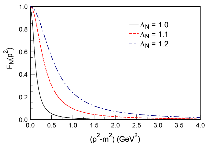
The contribution to the current matrix element given by (21), represented by Fig. 2b, involves a principal value integral over off-mass-shell momenta for one leg of the scattering amplitude. The proton propagator for this leg contains only the positive energy contribution. Determination of the off shell behavior of the scattering amplitude requires a dynamical model of the amplitude. Such a model is not currently available to us in the range of energies required for the experiments being performed at Jefferson Lab. In order to estimate the possible effects of this contribution to the current matrix elements, we use a simple prescription for the off-shell behavior of the amplitude. Although additional invariants are possible when the nucleon is allowed to go off shell, we keep only the forms in (23). The center-of-momentum angle is calculated using

\displaystyle{\cos\theta=\frac{t-u}{\sqrt{s-4m^{2}}\sqrt{\frac{(4m^{2}-t-u)^{2}}{s}-4m^{2}}}}

(26)

The invariants are then replaced by

\mathcal{F}_{i}(s,t)\rightarrow\mathcal{F}_{i}(s,t,u)F_{N}(s+t+u-3m^{2})

(27)

where

F_{N}(p^{2})=\frac{(\Lambda_{N}^{2}-m^{2})^{2}}{(p^{2}-m^{2})^{2}+(\Lambda_{N}^{2}-m^{2})^{2}}

(28)

and the $\mathcal{F}_{i}(s,t,u)$ are obtained from interpolation of the on-shell invariant functions with the center-of-momentum angle obtained from (26). The form factor (28) was used as a cutoff in calculating the Gross vertex function used in this paper with $\Lambda_{N}=1.675$ GeV. However, there should be an intrinsic fall off of the scattering amplitude due to the dynamics of the scattering which would be expected to be faster than provided by this cutoff mass. Figure 3 shows the off-shell form factor for cutoff masses of $\Lambda_{N}=$ 1.0, 1.1 and 1.2 GeV. In the absence of a dynamical model of the scattering amplitudes, the effect of possible off-shell contributions on various observables can be reasonably estimated by using cutoff masses in this range.

The contribution to the current matrix elements from (22), represented by Fig. 2c, contains the effect of negative energy propagation of the off-shell leg of the scattering amplitude. Since the denominator of this part of the propagator will be large compared with that of the positive energy part at large momentum transfers, we neglect this contribution for the present. This is the only approximation involved in our calculation. Note, however, that by dropping this contribution the current matrix elements are no longer covariant. We have chosen to calculate the matrix elements in the laboratory frame.

II.1 Differential Cross Section

The $D(e,e^{\prime}p)$ cross section for unpolarized deuterons and protons in the lab frame can be written as [34, 35]

$\displaystyle\left(\frac{d\sigma^{5}}{d\epsilon^{\prime}d\Omega_{e}d\Omega_{p}}\right)_{h}$	$\displaystyle=$	$\displaystyle\frac{m_{p}\,m_{n}\,p_{p}}{8\pi^{3}\,M_{d}}\,\sigma_{Mott}\,f_{rec}^{-1}\,$	(29)
		$\displaystyle\Big[\left(v_{L}R_{L}+v_{T}R_{T}+v_{TT}R_{TT}\cos 2\phi_{p}+v_{LT}R_{LT}\cos\phi_{p}\right)$
		$\displaystyle+hv_{LT^{\prime}}R_{LT^{\prime}}\sin\phi_{p}\Big]\,,$

where $M_{d}$ , $m_{p}$ and $m_{n}$ are the masses of the deuteron, proton and neutron, $p_{p}=p_{1}$ and $\Omega_{p}$ are the momentum and solid angle of the ejected proton, $\epsilon^{\prime}$ is the energy of the detected electron and $\Omega_{e}$ is its solid angle. The helicity of the electron is denoted by $h$ . The Mott cross section is

\sigma_{Mott}=\left(\frac{\alpha\cos(\theta_{e}/2)}{2\varepsilon\sin^{2}(\theta_{e}/2)}\right)^{2}

(30)

and the recoil factor is given by

f_{rec}=\left|1+\frac{\omega p_{p}-E_{p}q\cos\theta_{p}}{M_{d}\,p_{p}}\right|\,.

(31)

The kinematic coefficients $v_{K}$ are

$\displaystyle v_{L}$	$\displaystyle=$	$\displaystyle\frac{Q^{4}}{q^{4}}$	(32)
$\displaystyle v_{T}$	$\displaystyle=$	$\displaystyle\frac{Q^{2}}{2q^{2}}+\tan^{2}\frac{\theta_{e}}{2}$	(33)
$\displaystyle v_{TT}$	$\displaystyle=$	$\displaystyle-\frac{Q^{2}}{2q^{2}}$	(34)
$\displaystyle v_{LT}$	$\displaystyle=$	$\displaystyle-\frac{Q^{2}}{\sqrt{2}q^{2}}\sqrt{\frac{Q^{2}}{q^{2}}+\tan^{2}\frac{\theta_{e}}{2}}$	(35)
$\displaystyle v_{LT^{\prime}}$	$\displaystyle=$	$\displaystyle-\frac{Q^{2}}{\sqrt{2}q^{2}}\tan\frac{\theta_{e}}{2}$	(36)

If the response tensor is defined as

W^{\mu\nu}=\frac{1}{3}\sum_{s_{1},s_{2},\lambda_{d}}\left<\bm{p}_{1}s_{1};\bm{p}_{2}s_{2}\right|J^{\mu}\left|\bm{P}\lambda_{d}\right>^{*}\left<\bm{p}_{1}s_{1};\bm{p}_{2}s_{2}\right|J^{\nu}\left|\bm{P}\lambda_{d}\right>

(37)

the response functions $R_{K}$ are defined by

$\displaystyle R_{L}$	$\displaystyle\equiv$	$\displaystyle W^{00}$
$\displaystyle R_{T}$	$\displaystyle\equiv$	$\displaystyle W^{11}+W^{22}=w_{1,1}+w_{-1,-1}$
$\displaystyle R_{TT}\cos 2\phi_{p}$	$\displaystyle\equiv$	$\displaystyle W^{22}-W^{11}=2\Re(w_{1,-1})$
$\displaystyle R_{LT}\cos\phi_{p}$	$\displaystyle\equiv$	$\displaystyle 2\sqrt{2}\,\Re(W^{01})=-2\Re(w^{0}_{1}-w^{0}_{-1})$
$\displaystyle R_{LT^{\prime}}\sin\phi_{p}$	$\displaystyle\equiv$	$\displaystyle-2\sqrt{2}\,\Im(W^{01})=-2\Re(w^{0}_{1}+w^{0}_{-1})\,,$	(38)

where

w_{\lambda^{\prime}_{\gamma},\lambda_{\gamma}}=\frac{1}{3}\sum_{s_{1},s_{2},\lambda_{d}}\left<\bm{p}_{1}s_{1};\bm{p}_{2}s_{2}\right|J_{\lambda^{\prime}_{\gamma}}\left|\bm{P}\lambda_{d}\right>^{*}\left<\bm{p}_{1}s_{1};\bm{p}_{2}s_{2}\right|J_{\lambda_{\gamma}}\left|\bm{P}\lambda_{d}\right>

(39)

and

w^{0}_{\lambda_{\gamma}}=\frac{1}{3}\sum_{s_{1},s_{2},\lambda_{d}}\left<\bm{p}_{1}s_{1};\bm{p}_{2}s_{2}\right|J^{0}\left|\bm{P}\lambda_{d}\right>^{*}\left<\bm{p}_{1}s_{1};\bm{p}_{2}s_{2}\right|J_{\lambda_{\gamma}}\left|\bm{P}\lambda_{d}\right>

(40)

with

J_{\pm 1}=\mp\frac{1}{\sqrt{2}}(J^{1}\pm J^{2})

(41)

For our calculations, we have chosen the following kinematic conditions: the z-axis is parallel to $\bm{q}$ , and the missing momentum is defined as $\bm{p}_{m}\equiv\bm{q}-\bm{p}_{1}=\bm{p}_{2}=\bm{p}_{n}$ .

II.2 Asymmetries

The representation of the cross section in terms of response functions is due to the mixed polarization of the virtual photon which varies with the electron kinematics and polarization. The transverse-transverse response function is the result of interference between the $\lambda_{\gamma}=\pm 1$ helicity states while the longitudinal-transverse response functions $R_{LT}$ and $R_{LT^{\prime}}$ are the result of interference between the deuteron charge and two linear combinations of the $\lambda_{\gamma}=\pm 1$ helicity states. As an alternative to a complete separation of the cross section into response functions, the interference response functions can be accessed through linear combinations of differential cross sections to produce three interference asymmetries defined as

A_{TT}=\frac{v_{TT}R_{TT}}{v_{L}R_{L}+v_{T}R_{T}}

(42)

A_{LT}=\frac{\sigma_{0}(0^{\circ})-\sigma_{0}(180^{\circ})}{\sigma_{0}(0^{\circ})+\sigma_{0}(180^{\circ})}=\frac{v_{LT}R_{LT}}{v_{L}R_{L}+v_{T}R_{T}+v_{TT}R_{TT}}

(43)

and

\displaystyle{A_{LT^{\prime}}=\frac{\sigma_{+1}(90^{\circ})-\sigma_{-1}(90^{\circ})}{\sigma_{+1}(90^{\circ})+\sigma_{-1}(90^{\circ})}=\frac{v_{LT^{\prime}}R_{LT^{\prime}}}{v_{L}R_{L}+v_{T}R_{T}-v_{TT}R_{TT}}}\,,

(44)

where, for conciseness,

\sigma_{h}(\phi_{p})\equiv\left(\frac{d\sigma^{5}}{d\epsilon^{\prime}d\Omega_{e}d\Omega_{p}}\right)_{h}

(45)

Note that while $A_{LT}$ can be obtained by measuring protons in the electron scattering plane symmetrically about the direction of the three-momentum transfer, the asymmetries $A_{TT}$ and $A_{LT^{\prime}}$ require measurements to be made out of the scattering plane. The asymmetry $A_{LT^{\prime}}$ is defined as an electron single spin asymmetry and can, therefore, be easily obtained by flipping the beam helicity. While $R_{L}$ and $R_{T}$ are independent of photon-helicity-dependent phases, the interference response functions are not. As a result, the interference response functions can be very sensitive to phase differences generated by non-nucleonic currents and final state interactions. This is particularly true of $R_{LT^{\prime}}$ which can be shown to be zero in the PWIA. The interference response function, $R_{LT}$ , is very sensitive to the relativity included in the current operator, due to the various interference contributions from the charge and transverse current operators [36].

The observable $A_{LT^{\prime}}$ has recently been measured in Jefferson Lab’s Hall B [17]. Due to the large solid angle coverage in Hall B, and the averaging over $\phi_{p}$ , the transverse-transverse interference response that is multiplied with a factor of $\cos(2\phi_{p})$ in the cross section, drops out of the measured asymmetry $A_{LT^{\prime}}$ [37]. Therefore, from now on in this paper, we calculate

\displaystyle{A_{LT^{\prime}}^{Hall\,B}=\frac{v_{LT^{\prime}}R_{LT^{\prime}}}{v_{L}R_{L}+v_{T}R_{T}}}\,.

(46)

The difference between the asymmetry calculated with and without $R_{TT}$ is very small in practice, due to the small size of the transverse-transverse response.

III Results

In this section, we discuss our numerical results for several observables. We will investigate the effect of the final state interactions (FSIs), and in particular, we will point out the contributions of spin-dependent FSIs, both the single-spin-flip contributions and the double-spin-flip contributions. We will also discuss the relative importance of on-shell and off-shell contributions to FSI.

III.1 Differential Cross Sections

III.1.1 Momentum Distributions

The most natural observable to investigate is the differential cross section. In Fig. 4 our calculations are compared to the published $D(e,e^{\prime}p)$ data from Jefferson Lab’s Hall A. The data from Ulmer et al. [20] are shown together with our PWIA, on-shell FSI, and full FSI curves as a function of the missing momentum $p_{m}$ . For all of the calculations in the paper we use the MMD [38] proton electromagnetic form factors. The data are presented as a reduced cross section, which is defined as

\sigma_{reduced}=\frac{d^{5}\sigma}{d\Omega_{e^{\prime}}d\Omega_{N}dE_{e^{\prime}}}\,\,\frac{M_{d}f_{rec}}{\sigma_{ep}m_{p}m_{n}p_{p}}\,.

(47)

At lower missing momenta, the effects of FSIs are small. For missing momenta larger than $p_{m}\approx 110$ MeV, the FSI effects become visible. First, the PWIA curve is slightly above the FSI results, then, at $p_{m}\approx 300$ MeV, the FSI curves become larger than the PWIA contribution. The agreement with the data is quite nice overall. The off-shell FSI is small, and leads to final results a little below the data at larger missing momenta. This is a sensible result, as we do expect meson exchange currents (MECs) to play a role at the relatively low $Q^{2}$ at which these data were taken. Indeed, in [20], the calculation by Arenhoevel [39] agreed with the data at large missing momenta after MEC contributions were included; the FSI-only calculation was a bit below the data.

We also have added a panel with a linear plot of just the low missing momentum data. The full FSI curve and the on-shell FSI curve coincide in this region. It has been observed in several previous $D(e,e^{\prime}p)$ measurements that at very low missing momenta, the calculations are somewhat above the data. This is quite puzzling as at these low missing momenta, effects like FSIs, MECS etc are supposed to be small and well under control. For a nice compilation on this topic, see [21]. In [20], Fig. 1 shows the deviation of the reduced cross section data and the calculations. Here, we observe the same type of deviation at very low $p_{m}\leq 0.35~MeV$ . The largest discrepancy appears at $p_{m}=15~MeV$ , where our calculation overpredicts the data by $15\%$ . Overall, comparing with the previous results, our low missing momentum results seem to be an improvement, even though the discrepancy has not been fully removed. One main difference between the calculation presented in this article and the calculations in[20] is the fully relativistic approach we take here.

In Figure 5, the upper panel shows the cross section as a function of the missing momentum, with a beam energy of $5.5$ GeV, $Q^{2}=2~{\rm GeV}^{2}$ , $x_{Bj}=1$ , and $\phi_{p}=180^{\circ}$ . The choice of Bjorken-x implies roughly quasi-free kinematics. The azimuthal angle of the detected proton has been chosen to maximize the cross section. The PWIA and on-shell FSI curves are almost identical at very low missing momenta, up to $0.05$ GeV. Then, the FSI curve reduces the cross section compared to the PWIA result, roughly from $p_{m}=0.05$ GeV to $p_{m}=0.33$ GeV. For larger missing momenta, there is a marked increase in the differential cross section when FSI is included. These results are quite typical and have been seen in other calculations [40, 23, 26, 25]. The differential cross section decreases by several orders of magnitude with increasing missing momentum, and a small reduction due to FSI at lower missing momenta and larger differential cross section can lead to a very large increase at larger missing momenta and smaller differential cross sections. The inclusion of the off-shell FSI contributions leads to a slight reduction of the cross section for medium missing momenta.

The lower panel shows the ratios of the off-shell FSI calculations with $\Lambda_{N}=$ 1.0, 1.1 and 1.2 GeV to the on-shell FSI. The off-shell effects are small for small $p_{m}$ , but become increasingly large as $p_{m}$ increases. These effects are not particularly sensitive to the cutoffs chosen here, but must be quite sensitive to lower cutoff masses.

In Fig. 6, we investigate the role played by the various parts of the proton-neutron scattering amplitude contributing to (23). The dashed line shows the results without the three double-spin-flip terms in the amplitude. One can see that for missing momenta from $0.2$ GeV to $0.45$ GeV, the double-spin-flip contribution is quite relevant. Its omission in this region leads to a significantly smaller cross section. The single-spin-flip - or spin-orbit - part of the proton-neutron scattering amplitude becomes relevant only at higher missing momenta than the double-spin-flip terms. From roughly $p_{m}=0.3$ GeV on, omitting the spin-orbit contribution leads to a decrease in the differential cross section.

This clearly shows that while it is possible to parameterize the central part of the $NN$ scattering amplitude, and to reproduce the $NN$ cross section data this way, this type of parametrization effectively includes some physics that stems from the spin-dependent parts of the $NN$ amplitude. Here, it is interesting to see the influence of the spin-dependent parts of the $NN$ amplitude on the unpolarized cross section. While the logarithmic scale necessary for the momentum distribution conceals the effects, it is important to note that the relative importance of the spin-dependent FSI contributions changes with missing momentum. We will return to the effects of spin-dependent FSI with Fig. 10.

In Fig. 7, we display our results for the same four-momentum transfer, but higher $x_{Bj}=1.3$ . At this value of $x_{Bj}$ , and larger values, strong short-range $pn$ correlations have been reported by inclusive electron scattering experiments on deuterium [15, 41]. The deviation of the on-shell FSI from the PWIA is small for medium missing momenta, and seems to disappear altogether for missing momenta between 0.5 GeV and 0.6 GeV. However, the off-shell contribution to the FSI gains in relevance for larger missing momenta, and leads to a significant increase over the PWIA results at $p_{m}>0.4$ GeV. The lower panel again shows the ratio of off-shell FSI to the on-shell result for three values of the off-shell cutoff. The importance of the off-shell FSI here is larger than for $x_{Bj}=1$ (as discussed above when considering Fig. 5 and the sensitivity to the value of the cutoff is much greater. This is the expected behavior, as the deviation from $x_{Bj}=1$ corresponds to a deviation from the quasi-elastic kinematics, and stresses the off-shell region more. A recent new proposal [18] suggests a measurement of the cross section at somewhat larger $Q^{2}=3.5~{\rm GeV}^{2}$ , but the same value of $x_{Bj}=1.3$ and a beam energy of $E_{beam}=5.25$ GeV. The results of our calculation for these kinematics are similar to what is displayed above in Fig. 7. The on-shell FSI in this case deviates a bit more from the PWIA result than for the kinematics displayed here. The off-shell contribution is just as significant in the proposed kinematics.

III.1.2 Angular Distributions

In Figure 8, we show the cross section as a function of the angle $\theta_{m}$ of the missing momentum, with fixed $Q^{2}=2~{\rm GeV}^{2}$ and $p_{m}=0.4$ GeV. The beam energy and azimuthal angle of the proton are the same as for the momentum distribution graphs. The angular distribution of the cross section shows much less variation in the magnitude, and therefore can be shown on a linear plot, allowing for a better look at the relevance of various parts of the cross section. While the region beyond $\theta_{m}=80^{\circ}$ is kinematically accessible to experiment, a calculation in this region requires the knowledge of the $NN$ scattering amplitude above lab kinetic energies of $1.3$ GeV in the $pn$ system, which are not available from SAID. We therefore stay below $80^{\circ}$ . As is obvious from the plot, the most interesting features of the calculation are located below this angle: while the PWIA results are gently sloping upwards and then downwards for angles larger than $20^{\circ}$ , the FSI results initially follow this behavior, but then show a pronounced peak at around $\theta_{m}=70^{\circ}$ . This value corresponds to $x_{Bj}=1$ , i.e. quasi-free kinematics for the knocked-out nucleon. For the lower angles, the FSI simply leads to a reduction in the cross section, but the shape is unchanged. For larger angles, around $x_{Bj}=1$ , the diffractive nature of the FSI leads to a redistribution of strength from smaller missing momenta, causing a large peak.

If we consider the ratio of FSI to PWIA cross section, as is sometimes done when comparing various methods of calculation [23, 21], this ratio peaks at $70^{\circ}$ , too. Our calculation clearly shows the same shift from a peak at $90^{\circ}$ , as seen in Glauber theory calculations [42], to a lower angle, as seen in the Generalized Eikonal Approximation (GEA) [23] and the diagrammatic approach of Laget [26].

For the angular distribution, the influence of the off-shell FSI cut-off is clearly visible and can be studied easily. One does not expect a large contribution from far off-shell nucleons. The cut-off we use here serves to impose that constraint. For the kinematics displayed in Fig. 9, we investigate the effects of various cut-off values. The cut-off at $1$ GeV leads to a very small increase at small angles and a very small decrease at large angles, but the overall result is hardly different from the on-shell FSI only result. The primary effect for larger cutoff masses is to fill in the minimum in the on-shell result from $30^{\circ}$ to $65^{\circ}$ .

In Fig. 10, we show the effects of the various spin-dependent parts of the $pn$ scattering amplitude. It is very interesting to observe that in the peak region, the contribution of the spin-dependent FSIs (both single and double-spin-flip) amounts to about one quarter of the cross section. This is certainly a rather significant contribution. The contribution from the single-spin-flip term and the three double-spin-flip terms is about equal in the peak region. The figure shows that the double-spin-flip contribution to the cross section at small angles is almost negligible. It becomes noticeable at $\theta_{m}\approx 40^{\circ}$ , and then leads to a sizable increase of the differential cross section in the peak region. The omission of the single-spin-flip contribution leads to a noticeable reduction in the cross section for all angles. The effect is most pronounced in the peak region and in the very shallow dip just before the peak region.

To this point, we have considered the different contributions of the spin-dependent parts of the amplitude, i.e. of the $NN$ amplitude split up following the Saclay convention (24). Using the Saclay formalism with its classification according to the spin-dependence is quite useful, as it allows one to understand the new contributions from different parts of the current operator when adding the single-spin-flip term and the double-spin-flip terms, see [40]. Even though we did not rewrite our current operator to distinguish e.g. between magnetization current and convection current, seeing the $NN$ scattering amplitude in terms of its spin-dependence is a very natural view point, and allows for a certain intuitive understanding of the numerical results.

It is also interesting to investigate the $NN$ amplitude in terms of the five Fermi invariants, which are so practical for actual calculations. ¿From (56,70), it is clear that every invariant amplitude contains several different, spin-dependent pieces. In Fig. 11, we show the results of the calculation with on-shell FSI if only one of the five invariants is included. For comparison, the solid lines depicts the result obtained with the full $NN$ amplitude. The result obtained with just the pseudoscalar part is slightly above the full result for smaller angles, and continues smooth and almost straight towards larger angles. It does not exhibit a peak structure at large angles. The tensor and axial vector contributions are fairly close to the pseudoscalar contribution at large angles, and neither exhibits a peak at large angles. At small angles, however, these two contributions lead to a new peak, much larger than the original peak at large angles in the full result. The scalar and vector contributions show peaks at small angles, and a large peak at large angles. These results already show that there are large interference effects present between the various invariant amplitudes. There is no straightforward and intuitive explanation available for why these contributions interfere in such a way.

In Fig. 12, we show the angular distribution of the differential cross section for a lower missing momentum, $p_{m}=0.2$ GeV. The lower missing momentum implies that the limiting value of $1.3$ GeV lab energy for the $NN$ system is reached at larger angles than for $p_{m}=0.4$ GeV. While the PWIA curve here is very similar in shape to the curve at the higher missing momentum value, the FSI curve looks rather different now: instead of a fairly sharp peak around $\theta_{m}=70^{\circ}$ , we now observe a broad, shallow dip at larger angles. At lower missing momenta, the FSIs lead to a reduction in the cross section. Part of this strength is redistributed to larger missing momenta, as discussed above. Also including the off-shell FSIs has no effect at very small angles, roughly below $20^{\circ}$ , and then tends to shift the overall result towards lower angles.

In Fig. 13, the influence of the different kinds of FSIs is shown at low missing momentum. Switching off the double-spin-flip contribution leads to a small reduction in the cross section for medium and large angles, roughly $5\%$ in the region of the shallow dip. Switching off the single-spin-flip term, too, changes practically nothing. The FSIs in this kinematic region are overall smaller than for higher missing momenta. The influence of spin-dependent FSIs is smaller here, too. However, it is interesting to note that the double-spin-flip terms are actually more relevant here than the single-spin-flip terms. We have observed this already when discussing the momentum distributions shown in Fig. 6.

III.2 Asymmetries

Figure 14 shows the interference asymmetry $A_{TT}$ for $Q^{2}=2.0$ GeV and $E_{beam}=5.5$ GeV. The upper panel is for $x_{Bj}=1$ and the lower for $x_{Bj}=1.3$ .

In both cases, the FSI result in a substantial change from the PWIA result, both with respect to size and shape of the asymmetry. For $x_{Bj}=1$ , the variation with the cutoff mass for the three values shown here is small, but it is somewhat larger for $x_{Bj}=1.3$ reducing the asymmetry almost to zero for $\Lambda_{N}=1.2$ GeV around $p_{m}=0.5$ GeV.

Figure 15 shows results for the interference asymmetry $A_{LT}$ for the same kinematics as in the previous figure. Again the sensitivity to final state interactions is substantial. Sensitivity to off-shell contributions is relatively modest at $x_{Bj}=1$ but is much larger at $x_{Bj}=1.3$ .

The single-spin asymmetry $A_{LT^{\prime}}$ is shown in Fig. 16 for the same kinematics. This asymmetry is identically zero in the PWIA, so the FSI are responsible for any asymmetry. A more detailed discussion of FSI effects is given below for kinematics relevant to a recent experiment. Here, in these kinematics, we focus on comparing the behavior of the three asymmetries, in the same kinematics.

At $x_{Bj}=1$ there is very little sensitivity to off-shell contributions, but it is large at $x_{Bj}=1.3$ . As stated above, this behavior is expected as $x_{Bj}=1$ corresponds to quasi-free, i.e. on-shell, kinematics, while $x_{Bj}=1.3$ probes nucleons that are much more off-shell. From the plots for $x_{Bj}=1.3$ , one can see clearly that the off-shell contribution to the NN scattering amplitude introduces a certain amount of ambiguity, especially at medium to high missing momenta. While great progress has been made on the experimental side, with measurements at very high missing momenta, there clearly are some theoretical uncertainties in these kinematic regions.

We are in the fortunate situation that the asymmetry $A_{LT^{\prime}}$ has been measured over a wide range of kinematics, from very low four-momentum transfers $Q^{2}\approx 0.2~{\rm GeV}^{2}$ up to medium values of $Q^{2}\approx 1~{\rm GeV}^{2}$ [17]. The data are currently under analysis. In this range, the proton-neutron scattering amplitudes from SAID are available, so there are no limits to our ability to calculate for these kinematics.

Here, we discuss our results for two representative kinematics: $Q^{2}=0.5~{\rm GeV}^{2}$ , and $Q^{2}=1.0~{\rm GeV}^{2}$ . In both cases, we assume a beam energy of $2.558$ GeV. Fig. 17 shows our results for $Q^{2}=1~{\rm GeV}^{2}$ . The PWIA result is zero, and not shown on the plot. The full, on-shell FSI result starts out negatively, dips around $p_{m}\approx 0.25$ GeV, and then increases and changes sign around $p_{m}\approx 0.38$ GeV. Then, the asymmetry peaks around $p_{m}\approx 0.5$ GeV, and then decreases and changes sign again. The second zero of the asymmetry occurs at $p_{m}\approx 0.7$ GeV. One can see that the double-spin-flip contributions to the FSI are not very relevant: they just lead to small modifications in the dip and peak regions. The spin-orbit (i.e. the single-spin-flip) contribution is very important, though. Switching it off so that only the central FSI remains leads to a completely different picture: the asymmetry is tiny, and remains positive for large missing momenta.

In Fig. 18, we show the corresponding results for the spin-dependence of the FSIs for lower four-momentum transfer, $Q^{2}=0.5~{\rm GeV}^{2}$ . At these kinematics, we do expect the influence of meson exchange currents and isobar states to be relevant. These effects are not included in the present calculation. However, the FSIs are crucial for $A_{LT^{\prime}}$ , and we can investigate them within our model. The full calculations are qualitatively very similar at both $Q^{2}$ values, showing a negative dip around $p_{m}\approx 0.25$ GeV and then an increase into positive values, with a peak around $p_{m}\approx 0.5$ GeV. A very interesting difference, however, is the size of the contribution of the double-spin-flip terms to the FSI. While their influence is small, almost negligible, at the higher $Q^{2}$ value, it is quite significant for the low $Q^{2}$ value: the double-spin-flip terms serve to partially fill in the negative dip, and are also responsible for pushing the asymmetry back towards positive values.

III.3 FSI Details

One obvious difference between the calculation presented here and the traditional Glauber and generalized eikonal approximation (GEA) is the evaluation of the argument of the nucleon-nucleon scattering amplitude for the FSIs. As described in section II, we evaluate the five terms of the NN scattering amplitude(23) at the values of the Mandelstam variables $s$ and $t$ computed from the particular kinematics. In Glauber and GEA settings, one typically finds expressions where the NN scattering amplitude is evaluated assuming a purely transverse momentum transfer when evaluating $t$ , even though the longitudinal momentum transfer is taken into account in the GEA. This is typically denoted with expressions like $f_{NN}(k_{\perp})$ . With the kinematics variables as defined in Fig. 1, the Mandelstam $t$ is given by $t=(M_{d}-E_{k_{2}}+\omega-E_{p_{1}})^{2}-(\bf{p_{1}}+\bf{k_{2}}-\bf{q})^{2}$ , whereas assuming a purely transverse momentum transfer implies: $t_{\perp}=-(\bf{p_{1,\perp}}+\bf{k_{2,\perp}})^{2}$ . Using this we can define the cm scattering angle as

\cos\theta=1+\frac{2t_{\perp}}{s-4m^{2}}

(48)

In Fig. 19, we show the ratio of the transverse-momentum approximation to the full, on-shell calculation. The kinematics are identical to the kinematics used for Fig. 5: a beam energy of $5.5$ GeV, $Q^{2}=2~{\rm GeV}^{2}$ , $x_{Bj}=1$ , and $\phi_{p}=180^{\circ}$ . Up to missing momenta of $0.4$ GeV, the two approximation works well, leading to small deviations of less than $5\%$ . Beyond $0.4$ GeV, the deviation from the full result grows, and for missing momenta larger than $0.6$ GeV, the quality of the approximation deteriorates quickly.

We have performed the same calculation for the angular distribution shown in Fig. 8. Here, we found that the approximation does well - the deviations are less than $5\%$ for any angle. This corresponds to our findings for the momentum distribution.

As an illustrative example for the other observables discussed in this article, we also show our results for the asymmetry $A_{LT^{\prime}}$ in Fig. 20. The kinematics correspond to Fig. 17, we have used a beam energy of $2.558$ GeV and four-momentum transfer $Q^{2}=1~{\rm GeV}^{2}$ . The spike seen in the ratio around $p_{m}=0.4$ GeV stems from the sign change in the asymmetry, they are not relevant to our discussion. Again, we see that the approximation is doing well up to missing momenta of roughly $0.4$ GeV. Then, the approximation considerably overestimate the full result, and for very large missing momenta, $p_{m}\geq 0.7$ GeV, it even fails to reproduce the correct sign of the asymmetry. It is interesting to see that the effects of the approximation are visible even in a quantity that is a ratio of quantities that are both affected by the approximation.

In conclusion, approximating the argument of the NN scattering amplitude with the popular “transverse momentum transfer only” works well up to missing momenta of $0.4$ GeV for various observables. For missing momenta higher than that, the approximation becomes questionable.

IV Summary and Outlook

In this paper, we have presented a fully relativistic $D(e,e^{\prime}p)$ calculation in impulse approximation. We have steered clear from a number of common, simplifying assumptions. The only approximation made in this paper is neglecting the negative-energy contributions to the propagator of the off-shell nucleon. These contributions can realistically expected to be very small compared to the positive-energy contributions.

We have used a parametrization of experimental $NN$ data from SAID to describe the full $pn$ scattering amplitude for the final state interaction. This leads to certain limits in the kinematics we can access, as these parametrizations are available only for lab kinetic energies of $1.3$ GeV or less. In our calculations, we have investigated the effects of the different contributions to the NN scattering amplitude: the central, spin-orbit, and double-spin-flip parts, using the Saclay formalism to describe the different contributions. Many other fine calculations using the generalized eikonal approximation [23, 25, 24] or a diagrammatic approach [26] use the central part only. While the central part of the amplitude is clearly dominant in almost all observables, the spin-orbit and double-spin-flip parts do contribute visibly to the cross section in the peak area of the angular distribution, increasing the peak height roughly by a quarter. For the out-of-plane asymmetry $A_{LT^{\prime}}$ , which is non-zero only in the presence of FSIs, the spin-orbit part is clearly the most relevant. Depending on the kinematics, the double-spin-flip can also play a relevant role for this asymmetry.

We also showed the different contributions of the NN amplitude in terms of the five invariant amplitudes. Interestingly, they are all relevant, and a lot of interference effects contribute to the full result. It is not possible to identify a single, dominant contribution in this framework for the description of the NN amplitudes.

In the spirit of avoiding all unnecessary approximations, we have used the full argument for the calculation of the NN scattering amplitudes. In Glauber theory and its variants, one often encounters the assumption of a transverse momentum transfer only, and this changes the value of Mandelstam $t$ . We have investigated the validity of this assumption, and found that it is a very good approximation for missing momenta up to $0.4$ GeV. For higher missing momenta, the quality of this approximation deteriorates quickly, and it should probably not be used.

We have also compared the influence of the off-shell FSI contributions to the on-shell FSI contributions. The former are expected to not be too large, and they require some interpolation of on-shell amplitudes and the introduction of a regulator function to suppress very far off-shell contributions. The off-shell FSI contributions tend to be negligible to small for lower missing momenta, $p_{m}\leq 0.4$ GeV for any observable. Beyond that, their importance varies depending on the specific kinematics: the off-shell FSI is very small for the momentum distribution calculated for the quasi-free value $x_{Bj}=1$ , but it is large for $x_{Bj}=1.3$ . This pattern was observed both for the cross section and the asymmetries $A_{TT}$ , $A_{LT}$ , and $A_{LT^{\prime}}$ . The size of the off-shell contribution does depend on the chosen cut-off, with a larger cut-off admitting a sometimes much-larger contribution. The main purpose of showing figures with the ratios of off-shell calculations with different cut-offs to the on-shell result is to identify “safe” kinematics and observables, where the off-shell FSI contributions are definitely small. In regions where they are relevant, a certain amount of theoretical uncertainty cannot be avoided, until reliable and believable models of the off-shell NN interaction at the relevant energies are developed. This is particularly relevant for the interpretation of new data taken at high missing momentum at Jefferson Lab.

The current calculations will be applied or already have been applied to the forthcoming experimental data from Jefferson Lab [17, 14], and calculations for the BLAST data from MIT Bates [16] are planned. Our calculation also does a nice job of improving the agreement with the low missing momentum data of Ulmer et al. [20], even though the “low missing momentum puzzle” [21] is not completely resolved.

Logical next steps for enhancing our calculations are the inclusion of meson exchange currents, and isobar states.

Acknowledgments: We thank Paul Ulmer for quickly providing us with his data from [20] in tabulated form. SJ thanks Charlotte Elster for interesting discussions. This work was supported in part by funds provided by the U.S. Department of Energy (DOE) under cooperative research agreement under No. DE-AC05-84ER40150 and by the National Science Foundation under grants No. PHY-0354916 and PHY-0653312.

Appendix A Representations of the $NN$ amplitudes

The invariant functions $\mathcal{F}_{i}(s,t)$ can be obtained from scattering data. For example, the helicity amplitudes are defined as

\mathcal{M}_{\lambda_{1}^{\prime}\lambda_{2}^{\prime};\lambda_{1}\lambda_{2}}=(\bar{u}_{\lambda_{1}^{\prime}}(\bm{p}_{1}^{\prime}))_{a}(\bar{u}_{\lambda_{2}^{\prime}}(\bm{p}_{2}^{\prime}))_{b}M_{ab,cd}(u_{\lambda_{1}}(\bm{p}_{1}))_{c}(u_{\lambda_{2}}(\bm{p}_{2}))_{d}

(49)

where $u_{\lambda}(\bm{p})$ is the helicity spinor for helicity $\lambda$ . The helicity matrix elements for $pn$ scattering in the center-of-momentum frame can be obtained from the program SAID for laboratory kinetic energies of up to 1.3 GeV. If the amplitudes are extracted in units of $fm$ , the helicity amplitudes consistent with the conventions used here are related to the SAID amplitudes by

\mathcal{M}_{\lambda_{1}^{\prime}\lambda_{2}^{\prime};\lambda_{1}\lambda_{2}}=-\frac{4\pi\sqrt{s}}{\hbar cm^{2}}\mathcal{M}_{\lambda_{1}^{\prime}\lambda_{2}^{\prime};\lambda_{1}\lambda_{2}}^{SAID}\,.

(50)

Parity, time-reversal and particle interchange symmetries can be used to show that there are only five independent helicity amplitudes defined as

$\displaystyle a$	$\displaystyle=$	$\displaystyle\mathcal{M}_{1,1;1,1}$	(51)
$\displaystyle b$	$\displaystyle=$	$\displaystyle\mathcal{M}_{1,1;1,-1}$	(52)
$\displaystyle c$	$\displaystyle=$	$\displaystyle\mathcal{M}_{1,-1;1,-1}$	(53)
$\displaystyle d$	$\displaystyle=$	$\displaystyle\mathcal{M}_{1,1;-1,-1}$	(54)
$\displaystyle e$	$\displaystyle=$	$\displaystyle\mathcal{M}_{1,-1;-1,1}\,.$	(55)

Using (23) in (49) and solving for the invariant functions gives

\begin{pmatrix}\mathcal{F}_{S}\\ \mathcal{F}_{V}\ \\ \mathcal{F}_{T}\ \\ \mathcal{F}_{P}\ \\ \mathcal{F}_{A}\ \\ \end{pmatrix}=\frac{1}{s-4m^{2}}\begin{pmatrix}a_{11}&a_{12}&a_{13}&a_{14}&a_{15}\\ a_{21}&a_{22}&a_{23}&a_{24}&a_{25}\\ a_{31}&a_{32}&a_{33}&a_{34}&a_{35}\\ a_{41}&a_{42}&a_{43}&a_{44}&a_{45}\\ a_{51}&a_{52}&a_{53}&a_{54}&a_{55}\\ \end{pmatrix}\begin{pmatrix}a\\ b\\ c\\ d\\ e\\ \end{pmatrix}

(56)

where

$\displaystyle a_{11}$	$\displaystyle=$	$\displaystyle-a_{24}=a_{25}=-2a_{31}=a_{41}=-a_{54}=-a_{55}=-\frac{2m^{4}}{s}$	(57)
$\displaystyle a_{14}$	$\displaystyle=$	$\displaystyle-a_{15}=-a_{21}=-2a_{34}=2a_{35}=a_{44}=-a_{51}=\frac{2m^{4}}{s}-m^{2}$	(58)
$\displaystyle a_{12}$	$\displaystyle=$	$\displaystyle\frac{m[8m^{2}-(3+\cos\theta)s]}{\sqrt{s}\sin\theta}$	(59)
$\displaystyle a_{13}$	$\displaystyle=$	$\displaystyle\frac{m^{2}[2m^{2}(1+\cos\theta)-s(3+\cos\theta)]}{s(1+\cos\theta)}$	(60)
$\displaystyle a_{22}$	$\displaystyle=$	$\displaystyle\frac{4m^{2}(1+\cos\theta)}{\sqrt{s}\sin\theta}$	(61)
$\displaystyle a_{23}$	$\displaystyle=$	$\displaystyle\frac{2m^{2}[m^{2}(1+\cos\theta)+s]}{s(1+\cos\theta)}$	(62)
$\displaystyle a_{32}$	$\displaystyle=$	$\displaystyle-\frac{m\sqrt{s}(1-\cos\theta)}{2\sin\theta}$	(63)
$\displaystyle a_{33}$	$\displaystyle=$	$\displaystyle-\frac{m^{2}[m^{2}(1+\cos\theta)+s(1-\cos\theta)]}{s(1+\cos\theta)}$	(64)
$\displaystyle a_{42}$	$\displaystyle=$	$\displaystyle-\frac{m[8m^{2}+s(3+\cos\theta)]}{\sqrt{s}\sin\theta}$	(65)
$\displaystyle a_{43}$	$\displaystyle=$	$\displaystyle\frac{m^{2}[2m^{2}(1+\cos\theta)-s(3+\cos\theta)]}{s(1+\cos\theta)}$	(66)
$\displaystyle a_{45}$	$\displaystyle=$	$\displaystyle-\frac{m^{2}[2m^{2}(1-\cos\theta)+s(7+\cos\theta)]}{s(1-\cos\theta)}$	(67)
$\displaystyle a_{52}$	$\displaystyle=$	$\displaystyle-\frac{4m^{2}(1-\cos\theta)}{\sqrt{s}\sin\theta}$	(68)
$\displaystyle a_{53}$	$\displaystyle=$	$\displaystyle\frac{2m^{2}[m^{2}(1+\cos\theta)-s]}{s(1+\cos\theta)}\,.$	(69)

The Saclay amplitudes are given in terms of the helicity amplitudes by

\begin{pmatrix}a_{s}\\ b_{s}\\ c_{s}\\ d_{s}\\ e_{s}\\ \end{pmatrix}=\frac{1}{2\sqrt{2}}\begin{pmatrix}\cos\theta&-4\sin\theta&\cos\theta&\cos\theta&-\cos\theta\\ 1&0&1&-1&1\\ -1&0&1&1&1\\ 1&0&-1&1&1\\ -i\sin\theta&-4i\cos\theta&-i\sin\theta&-i\sin\theta&i\sin\theta\\ \end{pmatrix}\begin{pmatrix}a\\ b\\ c\\ d\\ e\\ \end{pmatrix}\,.

(70)

Equations (56) and (70) can then be used to obtain the transformation from the Saclay amplitudes to the Fermi invariant functions.

References

[1] M. Garcon and J. W. Van Orden, Adv. Nucl. Phys. 26, 293 (2001) [arXiv:nucl-th/0102049].
[2] R. A. Gilman and F. Gross, J. Phys. G 28, R37 (2002) [arXiv:nucl-th/0111015].
[3] I. Sick, Prog. Part. Nucl. Phys. 47, 245 (2001) [arXiv:nucl-ex/0208009].
[4] S. K. Bogner, R. J. Furnstahl and R. J. Perry, Phys. Rev. C 75, 061001 (2007) [arXiv:nucl-th/0611045].
[5] H. Hergert and R. Roth, Phys. Rev. C 75, 051001 (2007) [arXiv:nucl-th/0703006].
[6] F. Gross, J. W. Van Orden and K. Holinde, Phys. Rev. C 41, R1909 (1990); F. Gross, J. W. Van Orden and K. Holinde, Phys. Rev. C 45, 2094 (1992).
[7] The Deuteron Benchmarking Project, see http://hule.fiu.edu/highnp/deubenchmarking.htm
[8] Jefferson Lab Experiment E-94-017, spokespersons W. Brooks, M. Vineyard.
[9] A. Larson, G. A. Miller and M. Strikman, Phys. Rev. C 74, 018201 (2006) [arXiv:nucl-th/0604022].
[10] W. Cosyn, M. C. Martinez and J. Ryckebusch, arXiv:0710.4837 [nucl-th]; W. Cosyn, M. C. Martinez, J. Ryckebusch and B. Van Overmeire, Phys. Rev. C 74, 062201 (2006) [arXiv:nucl-th/0701029]; B. Van Overmeire and J. Ryckebusch, Phys. Lett. B 644, 304 (2007) [arXiv:nucl-th/0608040]; J. Ryckebusch, W. Cosyn, B. Van Overmeire and C. Martinez, Eur. Phys. J. A 31, 585 (2007).
[11] J. M. Laget, Phys. Rev. C 73, 044003 (2006); J. M. Laget, arXiv:nucl-th/0507035.
[12] B. Clasie et al., arXiv:0707.1481 [nucl-ex].
[13] J. Ryckebusch, W. Cosyn, B. Van Overmeire and C. Martinez, Eur. Phys. J. A 31, 585 (2007); J. Ryckebusch, P. Lava, M. C. Martinez, J. M. Udias and J. A. Caballero, Nucl. Phys. A 755, 511 (2005); P. Lava, M. C. Martinez, J. Ryckebusch, J. A. Caballero and J. M. Udias, Phys. Lett. B 595, 177 (2004) [arXiv:nucl-th/0401041]; L. L. Frankfurt, W. R. Greenberg, G. A. Miller, M. M. Sargsian and M. I. Strikman, Z. Phys. A 352, 97 (1995) [arXiv:nucl-th/9501009].
[14] Jefferson Lab Experiment E01 - 020, spokespersons W. Boeglin, M. Jones, A. Klein, P. Ulmer, J. Mitchell, E. Voutier.
[15] K. S. Egiyan et al. [CLAS Collaboration], Phys. Rev. Lett. 96, 082501 (2006) [arXiv:nucl-ex/0508026]; K. S. Egiyan et al. [CLAS Collaboration], Phys. Rev. C 68, 014313 (2003) [arXiv:nucl-ex/0301008].
[16] BLAST data from MIT Bates, Ph. D. thesis A. Maschinot (MIT 2005).
[17] G. Gilfoyle, spokesperson, Jefferson Lab Hall B, E5 run period; G.P. Gilfoyle, (the CLAS Collaboration), ’Out-of-Plane Measurements of the Fifth Structure Function of the Deuteron’, Bull. Am. Phys. Soc., Fall DNP Meeting, DF.00010(2006).
[18] W. Boeglin, spokesperson, proposal to Jefferson Lab PAC 33, 2007.
[19] A. Bussiere et al., Nucl. Phys. A 365, 349 (1981).
[20] P. E. Ulmer et al., Phys. Rev. Lett. 89, 062301 (2002).
[21] Werner Boeglin, talk at the 2005 Workshop on “Probing microscopic structure of the lightest nuclei in electron scattering at JLab energies and beyond”, Trento, Italy July 25-30, 2005, http://www.fiu.edu/ sargsian/ect05
[22] E. Voutier, arXiv:nucl-ex/0501020.
[23] M. M. Sargsian, Int. J. Mod. Phys. E 10, 405 (2001) [arXiv:nucl-th/0110053]; M. M. Sargsian, T. V. Abrahamyan, M. I. Strikman and L. L. Frankfurt, Phys. Rev. C 71, 044614 (2005) [arXiv:nucl-th/0406020]; L. L. Frankfurt, M. M. Sargsian and M. I. Strikman, Phys. Rev. C 56, 1124 (1997) [arXiv:nucl-th/9603018].
[24] J. Ryckebusch, D. Debruyne, P. Lava, S. Janssen, B. Van Overmeire and T. Van Cauteren, Nucl. Phys. A 728, 226 (2003) [arXiv:nucl-th/0305066]; D. Debruyne, J. Ryckebusch, W. Van Nespen and S. Janssen, Phys. Rev. C 62, 024611 (2000) [arXiv:nucl-th/0005058].
[25] C. C. degli Atti and L. P. Kaptari, Phys. Rev. C 71, 024005 (2005); C. Ciofi delgi Atti and L. P. Kaptari, arXiv:0705.3951 [nucl-th]; C. Ciofi degli Atti, L. P. Kaptari and D. Treleani, Phys. Rev. C 63, 044601 (2001) [arXiv:nucl-th/0005027].
[26] J. M. Laget, Phys. Lett. B 609, 49 (2005) [arXiv:nucl-th/0407072].
[27] R. Schiavilla, O. Benhar, A. Kievsky, L. E. Marcucci and M. Viviani, Phys. Rev. C72, 064003 (2005) [arXiv:nucl-th/0508048].
[28] B. Van Overmeire and J. Ryckebusch, Phys. Lett. B 650, 337 (2007) [arXiv:0704.0705 [nucl-th]].
[29] S. Jeschonnek, Phys. Rev. C 63, 034609 (2001) [arXiv:nucl-th/0009086].
[30] C. Ciofi degli Atti, L. P. Kaptari and H. Morita, Nucl. Phys. A 782, 191 (2007) [arXiv:nucl-th/0609029].
[31] F. Gross, Phys. Rev. 186, 1448 (1969); Phys. Rev. D 10, 223 (1974), Phys. Rev. C 26, 2203 (1982).
[32] J. W. Van Orden, N. Devine and F. Gross, Phys. Rev. Lett. 75, 4369 (1995).
[33] R. A. Arndt, W. J. Briscoe, I. I. Strakovsky and R. L. Workman, Phys. Rev. C 76, 025209 (2007) [arXiv:0706.2195 [nucl-th]]; data available through SAID, http://gwdac.phys.gwu.edu/
[34] A. S. Raskin and T. W. Donnelly, Ann. of Phys. 191, 78 (1989).
[35] V. Dmitrasinovic and F. Gross, Phys. Rev. C 40, 2479 (1989).
[36] S. Jeschonnek and T.W. Donnelly, Phys. Rev. C 57, 2438 (1998); S. Jeschonnek and J. W. Van Orden, Phys. Rev. C 62, 044613 (2000).
[37] G. Gilfoyle, private communication (e-mail October 2007).
[38] P. Mergell, Ulf-G. Meissner and D. Drechsel, Nucl. Phys. A 596, 367 (1996)
[39] H. Arenhoevel, W. Leidemann and E. L. Tomusiak, Phys. Rev. C 46, 455 (1992); H. Arenhovel, W. Leidemann and E. L. Tomusiak, Phys. Rev. C 52, 1232 (1995); W. Leidemann, E. L. Tomusiak and H. Arenhovel, Phys. Rev. C 43, 1022 (1991); F. Ritz, H. Goller, T. Wilbois and H. Arenhovel, Phys. Rev. C 55, 2214 (1997).
[40] S. Jeschonnek and T.W. Donnelly, Phys. Rev. C 59, 2676 (1999).
[41] E. Piasetzky, M. Sargsian, L. Frankfurt, M. Strikman and J. W. Watson, Phys. Rev. Lett. 97, 162504 (2006) [arXiv:nucl-th/0604012].
[42] A. Bianconi, S. Jeschonnek, N. N. Nikolaev and B. G. Zakharov, Phys. Lett. B343, 13 (1995); A. Bianconi, S. Jeschonnek, N. N. Nikolaev and B. G. Zakharov, Phys. Rev. C 53, 576 (1996). A. Bianconi, S. Jeschonnek, N. N. Nikolaev and B. G. Zakharov, Nucl. Phys. A608, 437 (1996).

A new calculation for D⁡(e,e′​p)​nD(e,e^{\prime}p)n at GeV energies

Abstract

pacs

I Introduction

II Theoretical Framework

II.1 Differential Cross Section

II.2 Asymmetries

III Results

III.1 Differential Cross Sections

III.1.1 Momentum Distributions

III.1.2 Angular Distributions

III.2 Asymmetries

III.3 FSI Details

IV Summary and Outlook

Appendix A Representations of the N​NNN amplitudes

References

A new calculation for $D(e,e^{\prime}p)n$ at GeV energies

Appendix A Representations of the $NN$ amplitudes