跳到论文正文
W Papers独立论文阅读器 arXiv:0805.3098 论文正文 计算阅读时间 · 0%
引用这篇论文根据当前论文元数据生成,正式投稿前建议核对。


License: arXiv.org perpetual non-exclusive license
arXiv:0805.3098v1 [hep-th] 20 May 2008

MPP-2008-38

UTHEP-562

May 2008

Bethe–Salpeter wave functions in integrable models

Sinya Aoki

Graduate School of Pure and Applied Sciences, University of Tsukuba

Ibaraki, 305-8571, Japan

Riken BNL Research Center, Upton, NY 11973, USA

Janos Balog

Research Institute for Particle and Nuclear Physics

1525 Budapest 114, Pf. 49, Hungary

Peter Weisz

Max-Planck-Institut für Physik

Föhringer Ring 6, D-80805 München, Germany

Abstract

We investigate some properties of Bethe–Salpeter wave functions in integrable models. In particular we illustrate the application of the operator product expansion in determining the short distance behavior. The energy dependence of the potentials obtained from such wave functions is studied, and further we discuss the (limited) phenomenological significance of zero–energy potentials.

1 Introduction

In a recent paper [1] which has received general recognition [2], Ishii, Hatsuda and one of the present authors (S. A) have presented results on the nucleon–nucleon (NN) potential from first principle lattice computations [3, 4]. The results qualitatively resemble phenomenological NN potentials which are employed in nuclear physics. The force at medium to long range (r≥1.2​fmr\geq 1.2{\rm fm}) is attractive; this feature which is essential for the existence of bound states of nuclei (e.g. the deuteron) has long well been understood in terms of pion and other heavier meson exchange. At short distances a characteristic repulsive core is produced [1] by the QCD dynamics, but this feature has not yet found a simpler theoretical explanation.

Intuitively the short distance behavior in QCD is encoded in operator product expansions (OPE). However wave functions and potentials in the framework of relativistic quantum field theory are notoriously “flexible” concepts. There are infinitely many definitions depending on the interpolating fields chosen and thus the universality of the short distance behavior extracted from one particular chosen wave function is not a priori clear. The wave function discussed in ref. [1] is a Bethe–Salpeter (BS) wave function with a particular nucleon interpolating field of lowest dimension. The phenomenological success of the results gives rise to the hope that one is on the “correct track”, however there remain many theoretical questions and refinements in the measurements to be made. For example the results are still in the quenched approximation, lattice artifacts must be studied in more detail, the dependence of the results on the interpolating field must be examined and the very definition of a potential via a BS wave function must be better understood.

It is our hope that studies of BS wave functions in integrable models in two dimensions will give us more insight into such questions. As an aside here we note that the methods used in ref. [1] were partially motivated by a method proposed to measure phase shifts in a two–dimensional model [5]. In this paper we investigate BS wave functions in the Ising model and in the O(3) non–linear sigma–model in two space–time dimensions.

In a remarkable paper, Fonseca and Zamolodchikov [6] obtained an exact expression for the BS wave function of the Ising field theory. In Sect. 2 we study its properties; in particular we can see at which distances the short distance behavior expected from the OPE sets in. We also point out that a zero energy potential defined from the BS wave function has a non-trivial form and may be a concept which may have a wider domain of applicability.

We further examine how the wave function in the Ising model is built from the contributions of the intermediate particle states. We find that intermediate states involving a relatively low number of particles give a good approximation down to quite short distances. This study was performed because in other integrable models the exact wave function is not (yet) known and the only analytical methods available are intermediate state approximations, the OPE (renormalized perturbation theory at short distances) and 1/n1/n expansions. As an example in Sect. 3 we study the (asymptotically free) O(3) sigma model in two dimensions.

Various technical details are relegated to appendices and in Sect. 4 we make some concluding remarks.

2 The two–dimensional Ising model in the scaling limit

In this section we will discuss properties of BS wave functions in the two–dimensional Ising field theory, but before introducing these we first briefly describe the theory and establish some notations and conventions.

The theoretical insight which is to be gained from the 2–d Ising model seems inexhaustible. In 1976 Wu, McCoy, Tracey and Barouch [7] showed that the model (at zero external field) has a continuum limit as one approaches the critical point. This relativistic quantum field theory, called the Ising field theory, describes on–shell free particles of mass M>0M>0. We denote the corresponding one–particle states with momentum p=M⁡(cosh⁡θ,sinh⁡θ)p=M(\cosh\theta,\sinh\theta) by |θ⟩|\theta\rangle, with state normalization

⟨θ′|θ⟩=4​π​δ​(θ−θ′).\langle\theta^{\prime}|\theta\rangle=4\pi\delta(\theta-\theta^{\prime})\,. (2.1)

The continuum limit of the spin field σ⁡(x)\sigma(x) is an interpolating field for this particle; we chose the normalization

⟨0|σ⁡(x)|θ⟩=e−i​p​x,p=M⁡(cosh⁡θ,sinh⁡θ).\langle 0|\sigma(x)|\theta\rangle={\rm e}^{-ipx}\,,\,\,\,\,\,\,p=M(\cosh\theta,\sinh\theta)\,. (2.2)

Although the theory has an alternative representation in terms of free (fermion) fields, the spin field is not a free field; nevertheless there is a wealth of information on its correlation functions. In ref. [7] it was shown that the two–point function of σ⁡(x)\sigma(x) satisfies the Painlevé III equation. More explicitly defining the vacuum 2–point function of σ⁡(x)\sigma(x) and also that of the corresponding disorder variable μ⁡(x)\mu(x) 11 1 which is local with respect to itself but non–local wrt σ⁡(x)\sigma(x) at equal times (which suffices for our considerations) by

G⁡(r)\displaystyle G(r) =\displaystyle= ⟨0|σ⁡((0,x1))​σ​(0)|0⟩,\displaystyle\langle 0|\sigma((0,x_{1}))\sigma(0)|0\rangle\,, (2.3)
G~​(r)\displaystyle\widetilde{G}(r) =\displaystyle= ⟨0|μ⁡((0,x1))​μ​(0)|0⟩,\displaystyle\langle 0|\mu((0,x_{1}))\mu(0)|0\rangle\,, (2.4)

where r=M​x1r=Mx_{1}. Then for the sum and difference

G±​(r)=G~​(r)±G⁡(r),G_{\pm}(r)=\widetilde{G}(r)\pm G(r)\,, (2.5)

one has

G±(r)=eχ⁡(r)/2e±φ(r)/2,G_{\pm}(r)={\rm e}^{\chi(r)/2}{\rm e}^{\pm\varphi(r)/2}\,, (2.6)

where the functions χ,φ\chi,\varphi obey the equations

1r​[r​φ′​(r)]′\displaystyle\frac{1}{r}[r\varphi^{\prime}(r)]^{\prime} =\displaystyle= 12​sh​(2​φ​(r)),\displaystyle\frac{1}{2}{\rm sh}(2\varphi(r))\,, (2.7)
1r​[r​χ′​(r)]′\displaystyle\frac{1}{r}[r\chi^{\prime}(r)]^{\prime} =\displaystyle= 12​[1−ch​(2​φ​(r))].\displaystyle\frac{1}{2}[1-{\rm ch}(2\varphi(r))]\,. (2.8)

For definiteness we are considering the theory obtained by taking the continuum limit from the symmetric phase, where μ⁡(x)\mu(x) has a non--vanishing vacuum expectation value 22 2 i.e. the fields σ,μ\sigma,\mu in Fonseca and Zamolodchikov [6] are interchanged with respect to ours. Also the field normalization differs..

The short and long distance behaviors of the functions φ,χ\varphi,\chi are summarized in Appendix A, and from these it follows that for small r>0r>0 (for the field normalization given in (2.2)),

G(r)∼Cχr−1/4+O(r3/4lnr),G(r)\sim C_{\chi}r^{-1/4}+{\rm O}(r^{3/4}\ln r)\,, (2.9)

(where the constant CχC_{\chi} is given in (A.99),) exhibiting the well known anomalous dimension of σ⁡(x)\sigma(x). For large distances r>0r>0 the correlation function falls exponentially:

G⁡(r)∼e−r8​π​r​[1+O⁡(r−1)].G(r)\sim\frac{{\rm e}^{-r}}{\sqrt{8\pi r}}\left[1+{\rm O}(r^{-1})\right]\,. (2.10)

The results on the 2–point function were subsequently derived in other ways (see e.g. [8] and [9]). A very elegant derivation recently presented by Fonseca and Zamolodchikov [6] is based on local conservation laws of the doubled Ising field theory.

2.1 Bethe–Salpeter wave functions

In their remarkable paper Fonseca and Zamolodchikov [6] showed that their methods also lead to exact results for a larger class of correlation functions. In particular they obtained exact expressions for the BS wave functions for 2–particle in–states

Ψ⁡(r,θ)\displaystyle\Psi(r,\theta) =\displaystyle= i​⟨0​|σ⁡((0,x1))​σ​(0)|​θ,−θ⟩in,\displaystyle i\langle 0|\sigma((0,x_{1}))\sigma(0)|\theta,-\theta\rangle^{\rm in}\,, (2.11)
Ψ~​(r,θ)\displaystyle\widetilde{\Psi}(r,\theta) =\displaystyle= i​⟨0​|μ⁡((0,x1))​μ​(0)|​θ,−θ⟩in.\displaystyle i\langle 0|\mu((0,x_{1}))\mu(0)|\theta,-\theta\rangle^{\rm in}\,. (2.12)

In fact Fonseca and Zamolodchikov consider the wave functions for general space–time arguments of the fields but here we restrict ourselves to equal times. Without loss of generality we can consider the rapidity θ≥0\theta\geq 0 and in the following consider only r>0r>0 since locality (and parity invariance) imply

Ψ⁡(r,θ)=Ψ⁡(−r,θ).\Psi(r,\theta)=\Psi(-r,\theta)\,. (2.13)

For the sum and difference

Ψ±=Ψ~±Ψ,\Psi_{\pm}=\widetilde{\Psi}\pm\Psi\,, (2.14)

Fonseca and Zamolodchikov [6] obtain

Ψ±​(r,θ)=G±​(r)ch​θ​[e−θ​Φ±​(r,θ)2−eθ​Φ∓​(r,θ)2],\Psi_{\pm}(r,\theta)=\frac{G_{\pm}(r)}{{\rm ch}\theta}\left[{\rm e}^{-\theta}\Phi_{\pm}(r,\theta)^{2}-{\rm e}^{\theta}\Phi_{\mp}(r,\theta)^{2}\right]\,, (2.15)

where G±G_{\pm} are defined in (2.5) and Φ±\Phi_{\pm} 33 3 which are the functions Ψ±\Psi_{\pm} in the notation of ref. [6], satisfy the coupled equations

Φ±′​(r,θ)=12​sh​(φ⁡(r)±θ)​Φ∓​(r,θ),\Phi^{\prime}_{\pm}(r,\theta)=\frac{1}{2}{\rm sh}(\varphi(r)\pm\theta)\Phi_{\mp}(r,\theta)\,, (2.16)

and the boundary conditions for small rr are

eχ⁡(r)/2Φ±(r,θ)∼2​πCχe±θ/2r1/4[1+O(r2lnr)].{\rm e}^{\chi(r)/2}\Phi_{\pm}(r,\theta)\sim\sqrt{2\pi}C_{\chi}{\rm e}^{\pm\theta/2}r^{1/4}\left[1+{\rm O}(r^{2}\ln r)\right]\,. (2.17)

In terms of these functions the BS wave function Ψ\Psi is given by

Ψ⁡(r,θ)=eχ⁡(r)/2ch​θ​[Φ+​(r,θ)2​cosh⁡(φ⁡(r)2−θ)−Φ−​(r,θ)2​cosh⁡(φ⁡(r)2+θ)].\Psi(r,\theta)=\frac{{\rm e}^{\chi(r)/2}}{{\rm ch}\theta}\left[\Phi_{+}(r,\theta)^{2}\cosh\left(\frac{\varphi(r)}{2}-\theta\right)-\Phi_{-}(r,\theta)^{2}\cosh\left(\frac{\varphi(r)}{2}+\theta\right)\right]\,. (2.18)

For short distances rr it has the expansion

Ψ⁡(r,θ)\displaystyle\Psi(r,\theta) ∼\displaystyle\sim Ψas​(r,θ)+O⁡(r7/4),\displaystyle\Psi_{\rm as}(r,\theta)+{\rm O}(r^{7/4})\,,\,\,\,\,\, (2.19)
Ψas​(r,θ)\displaystyle\Psi_{\rm as}(r,\theta) =\displaystyle= 2​π​Cχ​r3/4​sinh⁡θ,\displaystyle 2\pi C_{\chi}r^{3/4}\sinh\theta\,, (2.20)

which is as expected from the known operator expansion of the product of σ\sigma–fields

σ⁡((0,x1))​σ​(0)∼G⁡(r)+c​r3/4​ℰ​(0)+….\sigma((0,x_{1}))\sigma(0)\sim G(r)+cr^{3/4}{\cal E}(0)+.... (2.21)

where ℰ⁡(x){\cal E}(x) is the mass operator of dimension 1.

The coupled differential equations (2.7), (2.8), and (2.16) for Φ±,φ,χ\Phi_{\pm},\varphi,\chi with their known boundary conditions at r=0r=0 can be easily solved numerically. In Fig. 1 we depict the wave function Ψ⁡(r,θ)\Psi(r,\theta) for various rapidities, illustrating the early set in of the long distance sinusoidal behavior. Fig. 2 shows the wave function divided by sinh⁡θ\sinh\theta so that the leading short distance behaviors are the same, (see (2.20)); once this renormalization is done there is rather little remaining variation with the energy for r<0.5r<0.5; moreover the leading OPE behavior dominates up to r∼0.2r\sim 0.2.

Refer to caption
Figure 1: The Ising BS wave function Ψ⁡(r,θ)\Psi(r,\theta) for θ=1.0\theta=1.0 (dotted), θ=0.6\theta=0.6 (dot-dashed), θ=0.3\theta=0.3 (dashed), and the zero-energy wave function ℓ⁡(r)\ell(r) defined in Appendix B (solid).
Refer to caption
Figure 2: A renormalized Ising BS wave function Ψ⁡(r,θ)/sinh⁡(θ)\Psi(r,\theta)/\sinh(\theta) for for θ=0\theta=0 (top), θ=0.3,0.6,1.0\theta=0.3,0.6,1.0 (bottom solid curve). The leading short distance OPE behavior 2​π​Cχ​r3/42\pi C_{\chi}r^{3/4} (see (2.20)) is given by the dashed curve.
Refer to caption
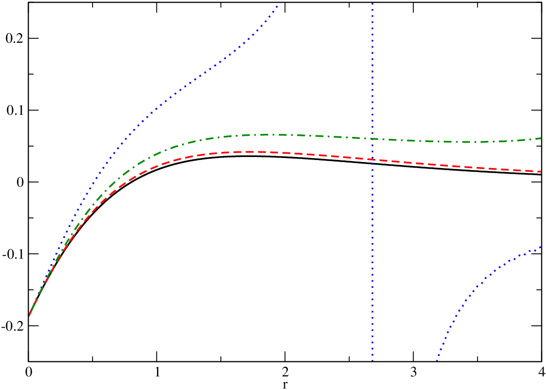
Figure 3: The Ising BS potentials (multiplied by r2r^{2}) r2​Vθ​(r)r^{2}V_{\theta}(r) for θ=1.0\theta=1.0 (dotted), θ=0.6\theta=0.6 (dot-dashed), θ=0.3\theta=0.3 (dashed), and θ=0\theta=0 (solid).

2.2 BS Potentials

From the BS wave function one can define a rapidity–dependent potential by

Vθ​(r):=Ψ′′​(r,θ)+sinh2⁡θ​Ψ​(r,θ)Ψ⁡(r,θ).V_{\theta}(r):=\frac{\Psi^{\prime\prime}(r,\theta)+\sinh^{2}\theta\Psi(r,\theta)}{\Psi(r,\theta)}\,. (2.22)

This definition is a direct analogy to that of energy dependent NN potentials made in ref. [1]. The hope is that for low energies and for the distances relevant for phenomenology the potentials are only mildly energy dependent 44 4 Of course this excludes distances near and beyond the point where Ψ⁡(r,θ)\Psi(r,\theta) has its first zero and hence at which Vθ​(r)V_{\theta}(r) is singular.. It is such an ansatz which seems to qualitatively apply in the NN case. We can investigate this question for the Ising field theory and find indeed only moderate variations in a reasonable range of parameters, as is illustrated in Fig. 3. The potential for θ=1.0\theta=1.0 becomes singular already at r∼2.681r\sim 2.681 where the corresponding wave function has its first node. Of course the physics in the Ising model is vastly different from the NN case, in particular in the Ising field theory there are no bound states.

The paper ref. [3] describes some ideas to obtain a local energy independent potential from the BS wave functions and this will hopefully be elucidated in our next paper [10]. Here we remark that a natural candidate for a potential of limited phenomenological relevance, as we will discuss below, is the zero–energy potential, obtained as the zero energy limit V0​(r)V_{0}(r) of (2.22). For purposes of numerical evaluation in the Ising model this can be expressed in terms of φ,χ\varphi,\chi (see Appendix A). A plot of this potential is included in Fig. 3. The asymptotic behaviors are analytically directly obtained from the formulae in Appendix A. From the large rr behavior of the zero energy wave function

Ψ0​(r):=limθ→0[θ−1​Ψ​(r,θ)]∼2​r+2π​r​e−r​(1−178​r+…),\Psi_{0}(r):=\lim_{\theta\to 0}\left[\theta^{-1}\Psi(r,\theta)\right]\sim 2r+\sqrt{\frac{2}{\pi r}}{\rm e}^{-r}\left(1-\frac{17}{8r}+\dots\right)\,, (2.23)

follows the leading large rr asymptotics of the zero energy potential:

V0​(r)∼12​π​1r3/2​e−r​(1−98​r+…),V_{0}(r)\sim\frac{1}{\sqrt{2\pi}}\frac{1}{r^{3/2}}\,{\rm e}^{-r}\left(1-\frac{9}{8r}+\dots\right)\,, (2.24)

i.e. the potential falls exponentially to zero from above. On the other hand for small rr using (2.20) we have

V0​(r)∼−316​1r2.V_{0}(r)\sim-\frac{3}{16}\frac{1}{r^{2}}\,. (2.25)

Since this potential is (classically) strongly attractive close to the origin the question of possible bound states naturally emerges. This would be fatal for the hope that the zero–energy potential is at all relevant for the Ising field theory. In Appendix A we show that indeed there are no bound states because (2.25) is not attractive enough in the quantum theory.

In Appendix B we consider the zero–energy potential in a slightly more general context. There we show that it reproduces the correct scattering length, which parameterizes the leading low momentum behavior of the phase shift. However in general it does not yield the exact next-to-leading behavior (although it may in some cases be a good approximation to it).

2.3 Intermediate particle state approximations to Ψ⁡(r,θ)\Psi(r,\theta)

In the Ising field theory we are, as discussed above, fortunate to have exact partial differential equations for the BS wave functions. However for most other integrable models this is not (yet) the case, and we have to resort to approximations in order to obtain quantitative results. One approach is to compute contributions from intermediate states from knowledge of the form factors. For the two–point function this approximation has been investigated in ref. [11], and there the contributions of only a few states is found to approximate the exact result down to very small distances where the OPE can be applied.

In the Hilbert space of in–states defined by the spin field the S–matrix operator is given by

𝐒=(−1)𝐍⁡(𝐍−1)/2,{\bf S}=(-1)^{{\bf N}({\bf N}-1)/2}\,, (2.26)

where 𝐍{\bf N} is the particle number operator. An energy independent phase is not observable in a scattering experiment; however the non-trivial S-matrix reflects the fact that σ⁡(x)\sigma(x) is not a free field.

Given knowledge of the S–matrix and assuming general properties such as analyticity and crossing symmetry (together with some additional technical assumptions) it was argued in ref. [12] that generalized form factors of the spin field are given by

⟨θ1,…,θt|σ(0)|θt+1,…,θn⟩inout\phantom{}{}^{\rm out}\langle\theta_{1},\dots,\theta_{t}|\sigma(0)|\theta_{t+1},\dots,\theta_{n}\rangle^{\rm in}
=(2​i)(n−1)/2​∏1≤i<j≤tT⁡(|θi−θj|)​∏1≤r≤t<s≤n𝒫T⁡(θr−θs)​∏t<k<l≤nT⁡(|θk−θl|),\displaystyle=(2i)^{(n-1)/2}\prod_{1\leq i<j\leq t}T(|\theta_{i}-\theta_{j}|)\prod_{1\leq r\leq t<s\leq n}\frac{\cal P}{T(\theta_{r}-\theta_{s})}\prod_{t<k<l\leq n}T(|\theta_{k}-\theta_{l}|)\,,

with nn an odd positive integer. 𝒫{\cal P} denotes the principle part and

T⁡(x)≡tanh⁡x2.T(x)\equiv\tanh\frac{x}{2}\,. (2.28)

Sandwiching a complete set of states

1=|0⟩⟨0|+∑r=1∞∫−∞∞d​θ14​π∫−∞θ1d​θ24​π…∫−∞θr−1d​θr4​π|θ1,…,θr⟩s⟨θ1,…,θr|s1=|0\rangle\langle 0|+\sum_{r=1}^{\infty}\int_{-\infty}^{\infty}\frac{{\rm d}\theta_{1}}{4\pi}\int_{-\infty}^{\theta_{1}}\frac{{\rm d}\theta_{2}}{4\pi}\dots\int_{-\infty}^{\theta_{r-1}}\frac{{\rm d}\theta_{r}}{4\pi}|\theta_{1},\dots,\theta_{r}\rangle^{\rm s}\phantom{}{}^{\rm s}\langle\theta_{1},\dots,\theta_{r}| (2.29)

(where s stands for in or out) between the fields, Ψ\Psi can be expressed as a sum over ss–particle contributions

Ψ⁡(r,θ)=∑s=1∞Ψ2​s−1​(r,θ).\Psi(r,\theta)=\sum_{s=1}^{\infty}\Psi_{2s-1}(r,\theta)\,. (2.30)

Starting with the 1–particle contribution we have

Ψ1​(r,θ)=−12​π​T​(2​θ)​p1​(r,θ).\Psi_{1}(r,\theta)=-\frac{1}{2\pi}T(2\theta)p_{1}(r,\theta)\,. (2.31)

with

p1​(r,θ)=∫−∞∞d​θ1​ei​r​sh​θ1​𝒫T⁡(θ1−θ)​T​(θ1+θ).p_{1}(r,\theta)=\int_{-\infty}^{\infty}{\rm d}\theta_{1}\,{\rm e}^{ir{\rm sh}\theta_{1}}\frac{{\cal P}}{T(\theta_{1}-\theta)T(\theta_{1}+\theta)}\,. (2.32)

Now use

𝒫T⁡(ϕ)=2​π​i​δ​(ϕ)+1T⁡(ϕ+i​ϵ),\frac{\cal P}{T(\phi)}=2\pi i\delta(\phi)+\frac{1}{T(\phi+i\epsilon)}\,, (2.33)

to obtain

p1=p1(2)+p1(1)+p1(0),p_{1}=p_{1}^{(2)}+p_{1}^{(1)}+p_{1}^{(0)}\,, (2.34)

where the superscripts denote the number of delta functions. So

p1(2)​(r,θ)\displaystyle p_{1}^{(2)}(r,\theta) =\displaystyle= (2​π​i)2​∫−∞∞d​θ1​ei​r​sh​θ1​δ​(θ1−θ)​δ​(θ1+θ)\displaystyle(2\pi i)^{2}\int_{-\infty}^{\infty}{\rm d}\theta_{1}\,{\rm e}^{ir{\rm sh}\theta_{1}}\delta(\theta_{1}-\theta)\delta(\theta_{1}+\theta) (2.35)
=\displaystyle= −2​π2​δ​(θ).\displaystyle-2\pi^{2}\delta(\theta)\,. (2.36)

Next

p1(1)​(r,θ)\displaystyle p_{1}^{(1)}(r,\theta) =\displaystyle= 2​π​i​∫−∞∞d​θ1​ei​r​sh​θ1​[δ⁡(θ1−θ)T⁡(θ1+θ+i​ϵ)+δ⁡(θ1+θ)T⁡(θ1−θ+i​ϵ)]\displaystyle 2\pi i\int_{-\infty}^{\infty}{\rm d}\theta_{1}\,{\rm e}^{ir{\rm sh}\theta_{1}}\left[\frac{\delta(\theta_{1}-\theta)}{T(\theta_{1}+\theta+i\epsilon)}+\frac{\delta(\theta_{1}+\theta)}{T(\theta_{1}-\theta+i\epsilon)}\right] (2.38)
=\displaystyle= 2​π​i​[ei​r​sh​θT⁡(2​θ+i​ϵ)−e−i​r​sh​θT⁡(2​θ−i​ϵ)]\displaystyle 2\pi i\left[\frac{{\rm e}^{ir{\rm sh}\theta}}{T(2\theta+i\epsilon)}-\frac{{\rm e}^{-ir{\rm sh}\theta}}{T(2\theta-i\epsilon)}\right]
=\displaystyle= 4​π2​δ​(θ)−4​π​sin⁡(r​sh​θ)T⁡(2​θ).\displaystyle 4\pi^{2}\delta(\theta)-4\pi\frac{\sin(r{\rm sh}\theta)}{T(2\theta)}\,. (2.39)

Finally

p1(0)​(r,θ)=∫−∞∞d​θ1​ei​r​sh​θ1​1T⁡(θ1−θ+i​ϵ)​T​(θ1+θ+i​ϵ).p_{1}^{(0)}(r,\theta)=\int_{-\infty}^{\infty}{\rm d}\theta_{1}\,{\rm e}^{ir{\rm sh}\theta_{1}}\frac{1}{T(\theta_{1}-\theta+i\epsilon)T(\theta_{1}+\theta+i\epsilon)}\,. (2.40)

Shifting the contour to the line parallel to the real axis with imaginary part i​π/2i\pi/2 (and observing that the contribution from the contours parallel to the imaginary axis at infinity is zero for r≠0r\neq 0) we get

p1(0)​(r,θ)\displaystyle p_{1}^{(0)}(r,\theta) =\displaystyle= −∫−∞∞dze−r​ch​z(ch​θ+i​sh​zch​θ−i​sh​z)\displaystyle-\int_{-\infty}^{\infty}{\rm d}z\,{\rm e}^{-r{\rm ch}z}\left(\frac{{\rm ch}\theta+i{\rm sh}z}{{\rm ch}\theta-i{\rm sh}z}\right) (2.41)
=\displaystyle= 2​K0​(r)−4​c​h2​θ​∫0∞d​z​e−r​ch​zch2​θ+sh2​z.\displaystyle 2K_{0}(r)-4{\rm ch}^{2}\theta\int_{0}^{\infty}{\rm d}z\,\frac{{\rm e}^{-r{\rm ch}z}}{{\rm ch}^{2}\theta+{\rm sh}^{2}z}\,. (2.42)

Summarizing we have

Ψ1​(r,θ)=12​π​[4​π​sin⁡(r​sh​θ)−T⁡(2​θ)​p1(0)​(r,θ)].\Psi_{1}(r,\theta)=\frac{1}{2\pi}\left[4\pi\sin(r{\rm sh}\theta)-T(2\theta)p_{1}^{(0)}(r,\theta)\right]\,. (2.43)

The plane wave part is as expected for a two particle S–matrix equal to −1-1; and p1(0)​(r,θ)p_{1}^{(0)}(r,\theta) decays exponentially as r→∞r\to\infty. However Ψ1​(r,θ)\Psi_{1}(r,\theta) diverges logarithmically as r→0r\to 0:

Ψ1​(r,θ)∼1π​T​(2​θ)​[ln⁡r+f⁡(θ)+O⁡(r)],\Psi_{1}(r,\theta)\sim\frac{1}{\pi}T(2\theta)\left[\ln r+f(\theta)+{\rm O}(r)\right]\,, (2.44)

which is very different from the short distance behavior of the exact wave function given in (2.20).

The contribution from the 3–particle states can be computed similarly. Here we just note that all contributions vanish exponentially as r→∞r\to\infty (some only as e−r{\rm e}^{-r} due to disconnected contributions). We have numerically computed these contributions for various rapidities and as a typical result we give the results for rapidity θ=0.3\theta=0.3 in Table 1 where we compare the approximations to the exact wave function. We observe that whereas (for this rapidity) the 1–particle approximation fails quite badly at r=0.1r=0.1, addition of the 3–particle contribution already makes the agreement much better at this distance and already here the asymptotic formula (2.20) which can be derived from the OPE sets in. Addition of the 5–particle intermediate states would of course improve the agreement to smaller distances as illustrated in the O(3) σ\sigma–model in the next section.

rr Ψ1​(r,0.3)\Psi_{1}(r,0.3) Ψ3​(r,0.3)\Psi_{3}(r,0.3) [Ψ1+Ψ3]​(r,0.3)[\Psi_{1}+\Psi_{3}](r,0.3) Ψ⁡(r,0.3)\Psi(r,0.3) Ψas​(r,0.3)\Psi_{\rm as}(r,0.3)
10.010.0 1.92482​e−1\phantom{-}1.92482{\rm e}-1 1.39916​e−61.39916{\rm e}-6 1.92484​e−1\phantom{-}1.92484{\rm e}-1 1.92484​e−11.92484{\rm e}-1
5.05.0 1.99793\phantom{-}1.99793 2.52957​e−42.52957{\rm e}-4 1.99818\phantom{-}1.99818 1.998181.99818
4.04.0 1.87759\phantom{-}1.87759 7.18688​e−47.18688{\rm e}-4 1.87831\phantom{-}1.87831 1.878311.87831
3.03.0 1.58539\phantom{-}1.58539 2.03727​e−32.03727{\rm e}-3 1.58743\phantom{-}1.58743 1.587431.58743
2.02.0 1.14970\phantom{-}1.14970 5.73985​e−35.73985{\rm e}-3 1.15544\phantom{-}1.15544 1.155441.15544
1.01.0 6.12374​e−1\phantom{-}6.12374{\rm e}-1 1.63733​e−21.63733{\rm e}-2 6.28747​e−1\phantom{-}6.28747{\rm e}-1 6.28748​e−16.28748{\rm e}-1
0.10.1 2.60053​e−4\phantom{-}2.60053{\rm e}-4 9.40535​e−29.40535{\rm e}-2 9.43136​e−2\phantom{-}9.43136{\rm e}-2 9.45618​e−29.45618{\rm e}-2 9.227​e−29.227{\rm e}-2
0.010.01 −2.43697​e−1-2.43697{\rm e}-1 2.50800​e−12.50800{\rm e}-1 7.10370​e−3\phantom{-}7.10370{\rm e}-3 1.64495​e−21.64495{\rm e}-2 1.641​e−21.641{\rm e}-2
0.0010.001 −4.59999​e−1-4.59999{\rm e}-1 3.85735​e−13.85735{\rm e}-1 −7.42642​e−2-7.42642{\rm e}-2 2.91863​e−32.91863{\rm e}-3 2.918​e−32.918{\rm e}-3
0.00010.0001 5.18897​e−45.18897{\rm e}-4 5.189​e−45.189{\rm e}-4
Table 1: Ψ⁡(r,θ)\Psi(r,\theta) the exact wave function, and Ψ1​(r,θ),Ψ3​(r,θ)\Psi_{1}(r,\theta),\Psi_{3}(r,\theta) the 1– and 3–particle contributions, and the leading short distance behavior Ψas​(r​θ)\Psi_{\rm as}(r\theta) given in (2.20), for θ=0.3\theta=0.3.

3 BS wave functions of the O(3) σ\sigma–model

In this section we will give a quantitative discussion of BS wave functions and their associated potentials in the O(3) non–linear sigma model in two dimensions. The O(nn) sigma model has long served as a favorite laboratory for testing ideas concerning asymptotically free theories [13, 14, 15, 16, 17]. Unfortunately there is in this case no exact expression known for correlation functions of any local operators. However for the case n=3n=3 the multi–particle form factors (FF) (defined in Eq. (3.61)) can be obtained recursively (although they become extremely complicated for higher particle states), and so one can often obtain excellent approximations to correlation functions in a wide range of energies by saturation with a low number of intermediate states.

The spectrum is considered to contain an O(nn) vector multiplet of particles of mass MM and to have no bound states. The two-particle S–matrix established by Zamolodchikov and Zamolodchikov [18] is given by:

Sa​b;c​d​(β)=∑I=02SI​(β)​PI​(a​b|c​d),S_{ab;cd}(\beta)=\sum_{I=0}^{2}S_{I}(\beta)P_{I}(ab|cd)\,, (3.45)

where β\beta is the rapidity difference of the incoming particles and PIP_{I} are ‘‘isospin” projectors given by 55 5 Note ∑e,fPI​(a​b|e​f)​PJ​(e​f|c​d)=δI​J​PI​(a​b|c​d),\sum_{e,f}P_{I}(ab|ef)P_{J}(ef|cd)=\delta_{IJ}P_{I}(ab|cd)\,, and for n=3n=3 one has ∑a,bPI​(a​b|a​b)=2​I+1.\sum_{a,b}P_{I}(ab|ab)=2I+1\,.

P0​(a​b|c​d)\displaystyle P_{0}(ab|cd) =\displaystyle= 1n​δa​b​δc​d,\displaystyle\frac{1}{n}\delta_{ab}\delta_{cd}\,, (3.46)
P1​(a​b|c​d)\displaystyle P_{1}(ab|cd) =\displaystyle= 12​δa​c​δb​d−12​δa​d​δb​c,\displaystyle\frac{1}{2}\delta_{ac}\delta_{bd}-\frac{1}{2}\delta_{ad}\delta_{bc}\,, (3.47)
P2​(a​b|c​d)\displaystyle P_{2}(ab|cd) =\displaystyle= 12​δa​c​δb​d+12​δa​d​δb​c−1n​δa​b​δc​d,\displaystyle\frac{1}{2}\delta_{ac}\delta_{bd}+\frac{1}{2}\delta_{ad}\delta_{bc}-\frac{1}{n}\delta_{ab}\delta_{cd}\,, (3.48)

and

SI​(β)=−(−1)I​e2​i​δI​(β).S_{I}(\beta)=-(-1)^{I}{\rm e}^{2i\delta_{I}(\beta)}\,. (3.49)

For the special case n=3n=3 the phase shifts are simply given by

δ0​(β)\displaystyle\delta_{0}(\beta) =\displaystyle= −arctan⁡(β2​π),\displaystyle-\arctan\left(\frac{\beta}{2\pi}\right)\,, (3.50)
δ2​(β)\displaystyle\delta_{2}(\beta) =\displaystyle= arctan⁡(βπ),\displaystyle\arctan\left(\frac{\beta}{\pi}\right)\,, (3.51)
δ1​(β)\displaystyle\delta_{1}(\beta) =\displaystyle= δ0​(β)+δ2​(β).\displaystyle\delta_{0}(\beta)+\delta_{2}(\beta)\,. (3.52)

We define BS wave functions as in the last section by

Ψa​b;c​d​(x1,θ)=⟨0​|σa​(0,x1)​σb​(0,0)|​c,θ;d,−θ⟩in,θ>0.\Psi_{ab;cd}(x_{1},\theta)=\langle 0|\sigma^{a}(0,x_{1})\sigma^{b}(0,0)|c,\theta;d,-\theta\rangle^{{\rm in}},\qquad\qquad\theta>0\,. (3.53)

The spin field σa​(x)\sigma^{a}(x) is an interpolating field for the massive particle and we fix the normalization by

⟨0​|σa​(0)|​b,θ⟩=δa​b.\langle 0|\sigma^{a}(0)|b,\theta\rangle=\delta^{ab}\,. (3.54)

Translation invariance and locality implies

Ψa​b;c​d​(−x1,θ)=Ψb​a;d​c​(x1,θ).\Psi_{ab;cd}(-x_{1},\theta)=\Psi_{ba;dc}(x_{1},\theta). (3.55)

Introducing isospin components TIT_{I} for all tensors Ta​b;c​dT_{ab;cd}\,:

TI=12​I+1​PI​(a​b|c​d)​Ta​b;c​d,T_{I}=\frac{1}{2I+1}P_{I}(ab|cd)T_{ab;cd}\,, (3.56)

Eq. (3.55) now implies

ΨI​(−x1,θ)=(−1)I​ΨI​(x1,θ).\Psi_{I}(-x_{1},\theta)=(-1)^{I}\Psi_{I}(x_{1},\theta)\,. (3.57)

As before the BS wave function can be expressed as an expansion over ss–particle contributions:

Ψa​b;c​d​(x1,θ)=∑s​oddΨa​b;c​d(s)​(x1,θ),\Psi_{ab;cd}(x_{1},\theta)=\sum_{s{\rm\,\,odd}}\Psi^{(s)}_{ab;cd}(x_{1},\theta)\,, (3.58)

and these can further be organized in contributions having specific large distance behavior. Since the computation is rather technical we relegate the details to Appendix C and here just summarize the result. Firstly it is convenient to introduce the modified wave function

Ψ~I​(r,θ)=itanh⁡θ​e−i​δI​(2​θ)​ΨI​(r/M,θ),\widetilde{\Psi}_{I}(r,\theta)=\frac{i}{\tanh\theta}{\rm e}^{-i\delta_{I}(2\theta)}\Psi_{I}(r/M,\theta)\,, (3.59)

since as shown in Appendix C Ψ~\widetilde{\Psi} becomes real (for real arguments). This WF has a (large distance) expansion which is naturally expressed in the form

Ψ~I​(r,θ)=∑m​odd{AI(m)​(r,θ)+BI(m)​(r,θ)},\widetilde{\Psi}_{I}(r,\theta)=\sum_{m{\rm\ odd}}\left\{A^{(m)}_{I}(r,\theta)+B^{(m)}_{I}(r,\theta)\right\}\,, (3.60)

where AI(m)​(r,θ)∼O⁡(e−m​r)A^{(m)}_{I}(r,\theta)\sim{\rm O}({\rm e}^{-mr}) and BI(m)​(r,θ)∼O⁡(e−(m−1)​r)B^{(m)}_{I}(r,\theta)\sim{\rm O}({\rm e}^{-(m-1)r}) for large rr. Their explicit expressions are given in Eqs. (C.173),(C.174) and involve integrals over products of the generalized form factors

⟨0​|σa​(0)|​b1,β1;…;bs,βs⟩in=ℱb1​…​bsa​(β1,…,βs),β1>β2>…​βs.\langle 0|\sigma^{a}(0)|b_{1},\beta_{1};\dots;b_{s},\beta_{s}\rangle^{\rm in}={\cal F}^{a}_{b_{1}\dots b_{s}}(\beta_{1},\dots,\beta_{s})\,,\,\,\beta_{1}>\beta_{2}>\dots\beta_{s}\,. (3.61)

From the connectivity properties of the matrix elements built of these form factors it follows that the ss–particle contribution (s≥3s\geq 3) contributes not only to A(s)A^{(s)} and B(s)B^{(s)} but also to A(s−2)A^{(s-2)}. The leading term is

BI(1)(r,θ)=2tanh⁡θ(−1)Isin{rsinhθ+δI(2θ)}.B^{(1)}_{I}(r,\theta)=\frac{2}{\tanh\theta}(-1)^{I}\sin\left\{r\sinh\theta+\delta_{I}(2\theta)\right\}\,. (3.62)

We have numerically computed the first 5 terms in the expansion for the three isospin values (in the case of O(3)) and a range of small (≤1.0\leq 1.0) rapidities. As for the case of the Ising model, we find that inclusion of sufficient number of terms in the long distance expansion gives a good description of the full wave function down to quite small distances. This is illustrated in Tables 3–5 in Appendix D where we give results for θ=0.3\theta=0.3. Although the individual terms diverge at short distances it seems that their sums are tending to zero in each channel see Figs 4–6. Exactly how the limit is reached can however not be read off from this approximation and we require a detailed OPE analysis which we will present in the next subsection.

Refer to caption
Figure 4: Contributions to the O(3) wave function in the I=0I=0 channel for θ=0.3\theta=0.3. The dotted curve is B0(1)​(r,0.3)B_{0}^{(1)}(r,0.3), the dashed curve is A0(1)​(r,0.3)A_{0}^{(1)}(r,0.3), the dot-dashed curve is B0(3)​(r,0.3)B_{0}^{(3)}(r,0.3), and the solid curve is the sum of the first 5 contributions in the long distance expansion.
Refer to caption
Figure 5: As in Fig. 4 but for I=1I=1.
Refer to caption
Figure 6: As in Fig. 4 but for I=2I=2.

As in the case of the Ising models the BS wave functions and their corresponding potentials are only weakly varying with the rapidity (for moderate rapidities) in the short to intermediate distance range.

Note for the zero energy WF we have

BI(1)​(r,0)=2​(−1)I​{r+aI},B^{(1)}_{I}(r,0)=2(-1)^{I}\left\{r+a_{I}\right\}\,, (3.63)

where

a0=−1π,a1=1π,a2=2π.a_{0}=-\frac{1}{\pi},\qquad\quad a_{1}=\frac{1}{\pi},\qquad\quad a_{2}=\frac{2}{\pi}\,. (3.64)

For large rr the potentials fall exponentially to zero; in particular for the zero energy potentials:

V0​(r)\displaystyle V_{0}(r) =\displaystyle= 118​2​π3r3​[1−0.615​r−1+O⁡(r−2)]​e−r,\displaystyle\phantom{-}\frac{1}{18}\sqrt{\frac{2\pi^{3}}{r^{3}}}\left[1-0.615r^{-1}+{\rm O}(r^{-2})\right]{\rm e}^{-r}\,, (3.65)
V1​(r)\displaystyle V_{1}(r) =\displaystyle= −136​2​π3r3​[1−0.056​r−1+O⁡(r−2)]​e−r,\displaystyle-\frac{1}{36}\sqrt{\frac{2\pi^{3}}{r^{3}}}\left[1-0.056r^{-1}+{\rm O}(r^{-2})\right]{\rm e}^{-r}\,, (3.66)
V2​(r)\displaystyle V_{2}(r) =\displaystyle= 118​2​π3r3​[1−1.570​r−1+O⁡(r−2)]​e−r.\displaystyle\phantom{-}\frac{1}{18}\sqrt{\frac{2\pi^{3}}{r^{3}}}\left[1-1.570r^{-1}+{\rm O}(r^{-2})\right]{\rm e}^{-r}\,. (3.67)

3.1 Operator product expansion

Consider the operator product

DIa​b​(y)=PI​(a​b|c​d)​(σc​(y)​σd​(0)),D^{ab}_{I}(y)=P_{I}(ab|cd)\left(\sigma^{c}(y)\sigma^{d}(0)\right)\,, (3.68)

for general n≥3n\geq 3. Using asymptotic freedom, we can show that its leading short distance expansion is of the form

D2a​b​(y)≈α⁡(|y|)​ta​b​(0)+…,D1a​b​(y)≈β⁡(|y|)​yμ​Jμa​b​(0)+…,D0a​b​(y)≈δa​bn​{γ0​(|y|)+|y|2​γ1​(|y|)​Θ​(0)+yμ​yν​γ2​(|y|)​T^μ​ν​(0)}+…\begin{split}D^{ab}_{2}(y)&\approx\alpha(|y|)\,t^{ab}(0)+\dots,\\ D^{ab}_{1}(y)&\approx\beta(|y|)\,y^{\mu}J^{ab}_{\mu}(0)+\dots,\\ D^{ab}_{0}(y)&\approx\frac{\delta^{ab}}{n}\Big\{\gamma_{0}(|y|)+|y|^{2}\gamma_{1}(|y|)\Theta(0)+y^{\mu}y^{\nu}\gamma_{2}(|y|)\widehat{T}_{\mu\nu}(0)\Big\}+\dots\\ \end{split} (3.69)

Here ta​bt^{ab} is a traceless iso–tensor operator of dimension 0, Jμa​bJ^{ab}_{\mu} is the Noether current and Θ\Theta and T^μ​ν\widehat{T}_{\mu\nu} is the (Lorentz) trace and traceless part of the energy–momentum tensor Tμ​νT_{\mu\nu}:

Θ=Tμμ,Tμ​ν=T^μ​ν+12​ημ​ν​Θ,\Theta=T^{\mu}_{\phantom{\mu}\mu},\qquad\quad T_{\mu\nu}=\widehat{T}_{\mu\nu}+\frac{1}{2}\eta_{\mu\nu}\Theta, (3.70)

η00=−η11=1\eta_{00}=-\eta_{11}=1. Finally the leading short distance behavior of the functions α⁡(|y|),β⁡(|y|),γj​(|y|)\alpha(|y|),\beta(|y|),\gamma_{j}(|y|) appearing in (3.69) can be computed in the framework of renormalized perturbation theory as discussed below.

Sandwiching the operator product between the vacuum and a two-particle state we have

⟨0​|DIa​b​(y)|​c,θ;d,−θ⟩in=PI​(a​b|c​d)​ΨI​(r,θ),\langle 0|D^{ab}_{I}(y)|c,\theta;d,-\theta\rangle^{\rm in}=P_{I}(ab|cd)\Psi_{I}(r,\theta)\,, (3.71)

where r=M​|y|r=M|y|.

Let us recall [19] the two–particle form factors of the operators occurring in the above short distance expansion:

⟨0​|ta​b​(0)|​c,α;d,β⟩in=(α−β−i​π)​tanh⁡(α−β2)​P2​(a​b|c​d),\langle 0|t^{ab}(0)|c,\alpha;d,\beta\rangle^{\rm in}=(\alpha-\beta-i\pi)\tanh\left(\frac{\alpha-\beta}{2}\right)P_{2}(ab|cd)\,, (3.72)
⟨0​|Jμa​b​(0)|​c,α;d,β⟩in=−i​π2​ϵμ​ν​qν​ψ​(α−β)​P1​(a​b|c​d),\langle 0|J^{ab}_{\mu}(0)|c,\alpha;d,\beta\rangle^{\rm in}=-i\pi^{2}\epsilon_{\mu\nu}q^{\nu}\psi(\alpha-\beta)P_{1}(ab|cd)\,, (3.73)
⟨0​|Tμ​ν​(0)|​a,α;b,β⟩in=π22​δa​b​(q2​ημ​ν−qμ​qν)​ψ⁡(α−β)α−β−i​π.\langle 0|T_{\mu\nu}(0)|a,\alpha;b,\beta\rangle^{\rm in}=\frac{\pi^{2}}{2}\delta^{ab}(q^{2}\eta_{\mu\nu}-q_{\mu}q_{\nu})\frac{\psi(\alpha-\beta)}{\alpha-\beta-i\pi}\,. (3.74)

Here

q0=M⁡(cosh⁡α+cosh⁡β),q1=M⁡(sinh⁡α+sinh⁡β),q^{0}=M(\cosh\alpha+\cosh\beta),\qquad\qquad q^{1}=M(\sinh\alpha+\sinh\beta)\,, (3.75)

ϵ01=−ϵ10=1\epsilon_{01}=-\epsilon_{10}=1 and

ψ⁡(θ)=θ−i​πθ⁡(2​π​i−θ)​tanh2⁡(θ2).\psi(\theta)=\frac{\theta-i\pi}{\theta(2\pi i-\theta)}\tanh^{2}\left(\frac{\theta}{2}\right)\,. (3.76)

Eq. (3.72) fixes the normalization of ta​bt^{ab}, which is otherwise undetermined.

Using these form factors, the leading short distance expansion of the isospin invariant wave functions are given as

Ψ2​(r,θ)≈α⁡(r)​(2​θ−i​π)​tanh⁡θ,Ψ1​(r,θ)≈r​β​(r)​i​π2​sinh⁡θ​tanh⁡θ2​θ​(i​π−θ)​(2​θ−i​π),Ψ0​(r,θ)≈(r​π)2​[2​γ1​(r)−γ2​(r)]​sinh2⁡θ4​θ​(i​π−θ),\begin{split}\Psi_{2}(r,\theta)&\approx\alpha(r)(2\theta-i\pi)\tanh\theta\,,\\ \Psi_{1}(r,\theta)&\approx r\beta(r)\frac{i\pi^{2}\sinh\theta\tanh\theta}{2\theta(i\pi-\theta)}(2\theta-i\pi)\,,\\ \Psi_{0}(r,\theta)&\approx(r\pi)^{2}[2\gamma_{1}(r)-\gamma_{2}(r)]\frac{\sinh^{2}\theta}{4\theta(i\pi-\theta)}\,,\\ \end{split} (3.77)

which in terms of the redefined (real) field Ψ~\widetilde{\Psi} in (3.59) read:

Ψ~2​(r,θ)≈α⁡(r)​π2+4​θ2,Ψ~1​(r,θ)≈r​β​(r)​π2​sinh⁡θ2​θ​π2+4​θ2π2+θ2,Ψ~0​(r,θ)≈(r​π)2​[2​γ1​(r)−γ2​(r)]​sinh⁡2​θ8​θ​1π2+θ2.\begin{split}\widetilde{\Psi}_{2}(r,\theta)&\approx\alpha(r)\sqrt{\pi^{2}+4\theta^{2}}\,,\\ \widetilde{\Psi}_{1}(r,\theta)&\approx r\beta(r)\frac{\pi^{2}\sinh\theta}{2\theta}\sqrt{\frac{\pi^{2}+4\theta^{2}}{\pi^{2}+\theta^{2}}}\,,\\ \widetilde{\Psi}_{0}(r,\theta)&\approx(r\pi)^{2}[2\gamma_{1}(r)-\gamma_{2}(r)]\frac{\sinh 2\theta}{8\theta}\frac{1}{\sqrt{\pi^{2}+\theta^{2}}}\,.\\ \end{split} (3.78)

We now outline the information which can be gained from perturbative field theory; for any undefined notation we refer the reader to [20]. We start with the short distance expansion

ΔIa​b​(y)=1g02​PI​(a​b|c​d)​Sc​(y)​Sd​(0)≈∑ωKI(ω)​(g0,y)​ℬI(ω)​a​b​(0)+…,\Delta^{ab}_{I}(y)=\frac{1}{g_{0}^{2}}P_{I}(ab|cd)S^{c}(y)S^{d}(0)\approx\sum_{\omega}K^{(\omega)}_{I}(g_{0},y){\cal B}^{(\omega)ab}_{I}(0)+\dots, (3.79)

where ℬI(ω)​a​b{\cal B}^{(\omega)ab}_{I} are (bare) local operators and the KI(ω)K^{(\omega)}_{I} are coefficient functions (which can, in principle, be calculated in perturbation theory). The operator product (3.68) differs by a (non–perturbative) rescaling from the renormalized version of (3.79):

Ωn−2​DIa​b​(y)=ΔI⁡(R)a​b​(y)=PI​(a​b|c​d)​S(R)c​(y)​S(R)d​(0)≈∑ωkI(ω)​(g,μ,y)​ℬI⁡(R)(ω)​a​b​(0),\begin{split}\Omega_{n}^{-2}D^{ab}_{I}(y)=\Delta^{ab}_{I(R)}(y)&=P_{I}(ab|cd)S^{c}_{(R)}(y)S^{d}_{(R)}(0)\\ &\approx\sum_{\omega}k^{(\omega)}_{I}(g,\mu,y){\cal B}^{(\omega)ab}_{I(R)}(0)\,,\\ \end{split} (3.80)

written in terms of renormalized operators ℬI⁡(R)(ω)​a​b{\cal B}^{(\omega)ab}_{I(R)} and finite coefficient functions kI(ω)k^{(\omega)}_{I}. The latter satisfies the renormalization group (RG) equation

{𝒟+γ⁡(g)+γI(ω)​(g)}​kI(ω)=0,\left\{{\cal D}+\gamma(g)+\gamma^{(\omega)}_{I}(g)\right\}k^{(\omega)}_{I}=0\,, (3.81)

where the RG γ\gamma–function

γI(ω)​(g)=γI​0(ω)​g2+…\gamma^{(\omega)}_{I}(g)=\gamma^{(\omega)}_{I0}g^{2}+\dots (3.82)

is related to the operator renormalization constant (in dimensional regularization) by

ZI(ω)=1−γI​0(ω)​g2ε+…,Z^{(\omega)}_{I}=1-\frac{\gamma^{(\omega)}_{I0}g^{2}}{\varepsilon}+\dots, (3.83)

corresponding to the operator ℬI(ω)​a​b{\cal B}^{(\omega)ab}_{I}\,.

In particular, for I=2I=2 we have only one operator

ℬ2a​b=τ~a​b=1g02​(Sa​Sb−1n​δa​b),{\cal B}_{2}^{ab}=\tilde{\tau}^{ab}=\frac{1}{g_{0}^{2}}\left(S^{a}S^{b}-\frac{1}{n}\delta^{ab}\right)\,, (3.84)

which has renormalization constant [20]

Z2=Zτ~=1+g2π​ε+…Z_{2}=Z_{\tilde{\tau}}=1+\frac{g^{2}}{\pi\varepsilon}+\dots (3.85)

and coefficient function

K2​(g0,y)=1+O⁡(g02).K_{2}(g_{0},y)=1+{\rm O}(g_{0}^{2})\,. (3.86)

Similarly, for I=1I=1 we have

B1​μa​b=Jμa​b,B^{ab}_{1\mu}=J^{ab}_{\mu}\,, (3.87)

with Z1=1Z_{1}=1 and

K1μ​(g0,y)=−12​yμ+O⁡(g02).K^{\mu}_{1}(g_{0},y)=-\frac{1}{2}y^{\mu}+{\rm O}(g_{0}^{2})\,. (3.88)

Finally for I=0I=0 we have the two operators

ℬ0(1)​a​b=δa​bn​Θ,ℬ0​μ​ν(2)​a​b=δa​bn​T^μ​ν{\cal B}_{0}^{(1)ab}=\frac{\delta^{ab}}{n}\Theta,\qquad\qquad{\cal B}_{0\mu\nu}^{(2)ab}=\frac{\delta^{ab}}{n}\widehat{T}_{\mu\nu} (3.89)

with Z0(ω)=1Z_{0}^{(\omega)}=1 (ω=1, 2\omega=1,\,2) and coefficient functions

K0(1)=C10​|y|2+O⁡(g02),K0(2)​μ​ν=−12​yμ​yν+O⁡(g02).K_{0}^{(1)}=C_{10}|y|^{2}+{\rm O}(g_{0}^{2}),\qquad\qquad K_{0}^{(2)\mu\nu}=-\frac{1}{2}y^{\mu}y^{\nu}+{\rm O}(g_{0}^{2})\,. (3.90)

Since Θ\Theta vanishes at tree level, the corresponding numerical coefficient C10C_{10} can only be determined by a one–loop calculation.

The equation (3.81) can be solved by standard RG methods. Introducing the running coupling function λ⁡(r)\lambda(r) as the solution of

1λ⁡(r)+χ​ln⁡λ⁡(r)=−ln⁡r,\frac{1}{\lambda(r)}+\chi\ln\lambda(r)=-\ln r\,, (3.91)

with χ=1/(n−2)\chi=1/(n-2) we find

α⁡(r)≈α0​λχ​{1+O⁡(λ)},β⁡(r)≈−12​Dn​(2​π​χ​λ)−χ​{1+O⁡(λ)},γ1​(r)≈C10​Dn​(2​π​χ​λ)−χ​{1+O⁡(λ)},γ2​(r)≈−12​Dn​(2​π​χ​λ)−χ​{1+O⁡(λ)}.\begin{split}\alpha(r)&\approx\alpha_{0}\,\lambda^{\chi}\left\{1+{\rm O}(\lambda)\right\}\,,\\ \beta(r)&\approx-\frac{1}{2}D_{n}\,(2\pi\chi\lambda)^{-\chi}\left\{1+{\rm O}(\lambda)\right\}\,,\\ \gamma_{1}(r)&\approx C_{10}D_{n}\,(2\pi\chi\lambda)^{-\chi}\left\{1+{\rm O}(\lambda)\right\}\,,\\ \gamma_{2}(r)&\approx-\frac{1}{2}D_{n}\,(2\pi\chi\lambda)^{-\chi}\left\{1+{\rm O}(\lambda)\right\}\,.\\ \end{split} (3.92)

The constant occurring in the coefficient α\alpha cannot be calculated since we do not know the relative normalization of the operator τ~(R)a​b\tilde{\tau}^{ab}_{(R)} with respect to ta​bt^{ab} whose normalization is fixed non-perturbatively by (3.72). We also do not know the numerical value of the non-perturbative constant DnD_{n} for general nn. However, we do know [20] D3=4/πD_{3}=4/\pi and this enables us to write for n=3n=3 (and, for simplicity, at zero energy):

Ψ~0​(r,0)≈r2π​λ​(C10+14)​{1+c0(1)​λ+…},Ψ~1​(r,0)≈−r2​λ​{1+c1(1)​λ+…},Ψ~2​(r,0)≈α0​π​λ​{1+c2(1)​λ+…}.\begin{split}\widetilde{\Psi}_{0}(r,0)&\approx\frac{r^{2}}{\pi\lambda}\left(C_{10}+\frac{1}{4}\right)\left\{1+c_{0}^{(1)}\lambda+\dots\right\}\,,\\ \widetilde{\Psi}_{1}(r,0)&\approx-\frac{r}{2\lambda}\left\{1+c_{1}^{(1)}\lambda+\dots\right\}\,,\\ \widetilde{\Psi}_{2}(r,0)&\approx\alpha_{0}\pi\,\lambda\left\{1+c_{2}^{(1)}\lambda+\dots\right\}\,.\\ \end{split} (3.93)

Here the O⁡(λ){\rm O}(\lambda) (and higher) corrections can in principle be calculated in higher orders of perturbation theory. The number C10C_{10} can also be obtained by a one–loop calculation. However, as explained above, the coefficient α0\alpha_{0} cannot be calculated by presently available methods.

Fortunately, the overall normalization cancels from the potential defined by

VI​(r)=Ψ~I′′​(r,0)Ψ~I​(r,0),V_{I}(r)=\frac{\widetilde{\Psi}^{\prime\prime}_{I}(r,0)}{\widetilde{\Psi}_{I}(r,0)}\,, (3.94)

and we find

V0​(r)≃2r2​{1−32​λ+O⁡(λ2)},V1​(r)≃−λr2​{1+[1−c1(1)]​λ+O⁡(λ2)},V2​(r)≃−λr2​{1−[1−c2(1)]​λ+O⁡(λ2)}.\begin{split}V_{0}(r)&\simeq\ \ \,\frac{2}{r^{2}}\left\{1-\frac{3}{2}\lambda+{\rm O}(\lambda^{2})\right\}\,,\\ V_{1}(r)&\simeq-\frac{\lambda}{r^{2}}\left\{1+\left[1-c_{1}^{(1)}\right]\lambda+{\rm O}(\lambda^{2})\right\}\,,\\ V_{2}(r)&\simeq-\frac{\lambda}{r^{2}}\left\{1-\left[1-c_{2}^{(1)}\right]\lambda+{\rm O}(\lambda^{2})\right\}\,.\\ \end{split} (3.95)

Note that for I=0I=0 we can calculate the first correction in λ⁡(r)\lambda(r) without knowledge of the O⁡(λ){\rm O}(\lambda) correction in (3.93).

rr 0.010.01 0.050.05 0.10.1 0.20.2
λ\lambda 0.1540.154 0.2220.222 0.2800.280 0.3930.393
Table 2: Values of λ⁡(r)\lambda(r).

In Fig. 7 we plot r2r^{2} times the potentials in the I=1,2I=1,2 channels obtained from the sum of the first 5 leading terms in the long distance (LD) expansions, together with the leading behavior (3.95) obtained from the OPE. They are plotted with respect to the variable λ\lambda defined in (3.91) (with χ=1\chi=1); in Table 2 we give some pairs of values (r,λ⁡(r))(r,\lambda(r)). We also plot the curve −λ+2​λ2-\lambda+2\lambda^{2} to illustrate that (“quite reasonable”) higher order expressions in the OPE expansion could be found to make smooth meetings with the LD approximations. We think that the 5–term LD approximation is accurate down to λ∼0.2\lambda\sim 0.2 (which already corresponds to quite short distances) in the I=1I=1 channel and even to smaller distances in the I=2I=2 channel. This can be monitored by studying the stability of successive LD approximations, including only 3 terms, 4 terms and 5 terms respectively. This is illustrated in Fig. 8 for I=1I=1. Alternativey one can appreciate the situation by inspecting Table 6 in Appendix D where we give the double derivatives of the separate contributions times r2r^{2} in the various channels.

Refer to caption
Figure 7: “Long distance approximation” to r2​V1​(r)r^{2}V_{1}(r) (solid) and r2​V2​(r)r^{2}V_{2}(r) (dashed). The lower dotted line is the leading short distance behavior −λ-\lambda and the upper dotted line is −λ+2​λ2-\lambda+2\lambda^{2}.
Refer to caption
Figure 8: Successive LD approximations to r2​V1​(r)r^{2}V_{1}(r); The dotted, dashed and solid lines correspond to approximations using 3,4,5 terms repectively.

Fig. 9 shows the zero-energy potential in the I=0I=0 channel. Here the LD breaks down already larger distances, in fact there is no stability in the sense described above even at r=0.1r=0.1. The figure however suggests that our 5–term approximation may still be quite good there, but it would need computation of higher order terms to confirm this. Never the less it is plausible that the approximation joins smoothly to the OPE expansion where again higher order terms are required to improve the quantitative picture.

Refer to caption
Figure 9: LD approximation to r2​V0​(r)r^{2}V_{0}(r) (solid). The upper dotted line is the leading short distance behavior and the lower dotted line is 2−3​λ−8​λ22-3\lambda-8\lambda^{2}.

4 Conclusions

In this paper we have investigated BS wave functions in integrable models; the Ising and O(3) σ\sigma–models. We have seen that potentials derived from them are rather slowly varying with energy in the short and intermediate distance range M​|x|<∼1M|x|<\sim 1. We have also discussed the relevance of the zero-energy potential and its phenomenological limitations. In these models we have found that a good approximation to the wave functions can be obtained by combining a long distance expansion (from contributions of intermediate states) and a short distance expansion from the OPE. It would be instructive to study some other examples in particular models with bound states.

Given a BS wave function constructed from a particular choice of local fields, it is clear that its short distance behavior can be obtained by an analysis of the OPE expansion. Further it follows from naive dimensional analysis that the BS potentials derived from (most) wave functions that vanish at the origin will behave as |x|−2|x|^{-2} (modified by logarithms). The overall sign in 3–dimensions indicates its attractive or repulsive nature. How this sign may depend on the particular interpolating field remains an important question.

In a sequel paper [10] we plan to include a more general discussion on potentials obtained from BS wave functions. We will also present OPE predictions for the short distance behaviors of BS wave functions (and the resulting short distance behavior of the potentials) for the pion–pion and nucleon–nucleon cases in QCD, for some choice of the interpolating fields..

Acknowledgments

J. B. and S. A. are grateful to the Max–Planck–Institut für Physik for its hospitality. This investigation was supported in part by the Hungarian National Science Fund OTKA (under T049495) and the Grant-in-Aid of the Japanese Ministry of Education (No. 20340047).

Appendix Appendix A

A.1 Asymptotic behaviors of the functions φ,χ\varphi,\chi

Note here we always take r>0r>0. The short distance behaviors of φ,χ\varphi,\chi are given by [6]:

e−φ⁡(r)\displaystyle{\rm e}^{-\varphi(r)} ∼\displaystyle\sim −12​r​Ω​(r)​[1+O⁡(r4)],\displaystyle-\frac{1}{2}r\Omega(r)\left[1+{\rm O}(r^{4})\right]\,, (A.96)
eχ⁡(r)\displaystyle{\rm e}^{\chi(r)} ∼\displaystyle\sim −2​Cχ2​r​Ω​(r)​[1+O⁡(r2)],\displaystyle-2C_{\chi}^{2}\sqrt{r}\Omega(r)\left[1+{\rm O}(r^{2})\right]\,, (A.97)

where

Ω⁡(r)=ln⁡(k​r),k=18​eγ,\Omega(r)=\ln(kr)\,,\,\,\,\,\,\,\,k=\frac{1}{8}{\rm e}^{\gamma}\,, (A.98)

where γ\gamma is the Euler–Mascheroni constant (=0.57721566490​…=0.57721566490\dots), and

Cχ=2−7/6A−3e1/4=0.27119012339…,C_{\chi}=2^{-7/6}A^{-3}{\rm e}^{1/4}=0.27119012339\dots\,, (A.99)

where AA is Glaisher’s constant:

A=exp⁡{112−ζ′​(−1)}=1.282427​…A=\exp\left\{\frac{1}{12}-\zeta^{\prime}(-1)\right\}=1.282427\dots (A.100)

Next for long distances [6]:

φ⁡(r)\displaystyle\varphi(r) =\displaystyle= 2π​K0​(r)+O⁡(e−3​r),\displaystyle\frac{2}{\pi}K_{0}(r)+{\rm O}({\rm e}^{-3r})\,, (A.101)
χ⁡(r)\displaystyle\chi(r) =\displaystyle= −2​ln⁡2−2​rπ2​[r⁡{K0​(r)2−K1​(r)2}+K0​(r)​K1​(r)]+O⁡(e−4​r).\displaystyle-2\ln 2-\frac{2r}{\pi^{2}}\left[r\{K_{0}(r)^{2}-K_{1}(r)^{2}\}+K_{0}(r)K_{1}(r)\right]+{\rm O}({\rm e}^{-4r})\,. (A.102)

Recall the modified Bessel function

K0​(r)\displaystyle K_{0}(r) =\displaystyle= ∫0∞d​z​e−r​ch​z,\displaystyle\int_{0}^{\infty}{\rm d}z\,{\rm e}^{-r{\rm ch}z}\,, (A.103)

behaves for small rr as

K0​(r)=−ln⁡(r2)−γ+O⁡(r2),K_{0}(r)=-\ln\left(\frac{r}{2}\right)-\gamma+{\rm O}(r^{2})\,, (A.104)

and for large rr,

K0​(r)=π2​r​e−r​[1−18​r+…],K_{0}(r)=\sqrt{\frac{\pi}{2r}}{\rm e}^{-r}\left[1-\frac{1}{8r}+\dots\right]\,, (A.105)

and K1​(r)=−K0′​(r)K_{1}(r)=-K_{0}^{\prime}(r)\,.

A.2 Zero–energy potential

Expanding Φ±​(r,θ)\Phi_{\pm}(r,\theta) for small θ\theta:

Φ±​(r,θ)=Φ0​(r)±θ​Φ1​(r)+…\Phi_{\pm}(r,\theta)=\Phi_{0}(r)\pm\theta\Phi_{1}(r)+\dots (A.106)

and defining

μ⁡(r)\displaystyle\mu(r) =\displaystyle= Φ0​(r)2,\displaystyle\Phi_{0}(r)^{2}\,, (A.107)
ν⁡(r)\displaystyle\nu(r) =\displaystyle= 2​Φ0​(r)​Φ1​(r),\displaystyle 2\Phi_{0}(r)\Phi_{1}(r)\,, (A.108)

we have

μ′​(r)\displaystyle\mu^{\prime}(r) =\displaystyle= μ⁡(r)​sinh⁡φ​(r),\displaystyle\mu(r)\sinh\varphi(r)\,, (A.109)
ν′​(r)\displaystyle\nu^{\prime}(r) =\displaystyle= μ⁡(r)​cosh⁡φ​(r).\displaystyle\mu(r)\cosh\varphi(r)\,. (A.110)

Then it follows for small θ\theta:

Ψ⁡(r,θ)∼2​θ​eχ⁡(r)/2​[ν⁡(r)​cosh⁡φ⁡(r)2−μ⁡(r)​sinh⁡φ⁡(r)2]+…\Psi(r,\theta)\sim 2\theta{\rm e}^{\chi(r)/2}\left[\nu(r)\cosh\frac{\varphi(r)}{2}-\mu(r)\sinh\frac{\varphi(r)}{2}\right]+\dots (A.111)

and

V0​(r):=limθ→0Ψ′′​(r,θ)Ψ⁡(r,θ)\displaystyle V_{0}(r):=\lim_{\theta\to 0}\frac{\Psi^{\prime\prime}(r,\theta)}{\Psi(r,\theta)}
=14​[χ′​(r)​(2r+χ′​(r))−φ′​(r)2]+F⁡(r)ν⁡(r)​cosh⁡φ⁡(r)2−μ⁡(r)​sinh⁡φ⁡(r)2.\displaystyle=\frac{1}{4}\left[\chi^{\prime}(r)\left(\frac{2}{r}+\chi^{\prime}(r)\right)-\varphi^{\prime}(r)^{2}\right]+\frac{F(r)}{\nu(r)\cosh\frac{\varphi(r)}{2}-\mu(r)\sinh\frac{\varphi(r)}{2}}\,. (A.112)

with

F⁡(r)=12​{χ′​(r)​φ′​(r)+φ′′​(r)}​{ν⁡(r)​sinh⁡φ⁡(r)2−μ⁡(r)​cosh⁡φ⁡(r)2}\displaystyle F(r)=\frac{1}{2}\left\{\chi^{\prime}(r)\varphi^{\prime}(r)+\varphi^{\prime\prime}(r)\right\}\left\{\nu(r)\sinh\frac{\varphi(r)}{2}-\mu(r)\cosh\frac{\varphi(r)}{2}\right\}
+μ⁡(r)​{χ′​(r)+sinh⁡φ⁡(r)}​cosh⁡φ⁡(r)2.\displaystyle+\mu(r)\left\{\chi^{\prime}(r)+\sinh\varphi(r)\right\}\cosh\frac{\varphi(r)}{2}\,. (A.113)

A.3 Absence of bound states

A bound state would have negative energy −E-E and would be a solution of the Schrödinger equation

−Φ′′+V0​Φ=−E​Φ,-\Phi^{\prime\prime}+V_{0}\Phi=-E\Phi\,, (A.114)

with large rr asymptotics

Φ⁡(r)∼e−E​r,\Phi(r)\sim{\rm e}^{-\sqrt{E}r}\,, (A.115)

i.e. would be normalizable.

It is important to impose the right boundary conditions at the origin. It turns out [21, 22] that the correct boundary condition is

Φ⁡(r)∼r3/4.\Phi(r)\sim r^{3/4}\,. (A.116)

In other words, the other, more singular solution of the Schrödinger equation, which would behave like

Φ⁡(r)∼r1/4\Phi(r)\sim r^{1/4} (A.117)

is not allowed (the Hamilton operator would not be self-adjoint).

Using this information it is easy to derive the formula

Ψ0′(r)Φ(r)−Ψ0(r)Φ′(r)=−E∫0rdxΦ(x)Ψ0(x).\Psi^{\prime}_{0}(r)\Phi(r)-\Psi_{0}(r)\Phi^{\prime}(r)=-E\int_{0}^{r}{\rm d}x\,\Phi(x)\Psi_{0}(x)\,. (A.118)

The left hand side vanishes for large rr and we know that the zero energy wave function Ψ0​(r)\Psi_{0}(r) (2.23) is positive everywhere. Therefore the bound state wave function has to change sign somewhere. We denote this point by r0r_{0} and assume Φ⁡(r)\Phi(r) is positive between the origin and this point. Then we have

−Ψ0(r0)Φ′(r0)=−E∫0r0dxΦ(x)Ψ0(x),-\Psi_{0}(r_{0})\Phi^{\prime}(r_{0})=-E\int_{0}^{r_{0}}{\rm d}x\,\Phi(x)\Psi_{0}(x)\,, (A.119)

implying that

Φ′​(r0)>0,\Phi^{\prime}(r_{0})>0\,, (A.120)

but this is obviously a contradiction, so Φ⁡(r)\Phi(r) cannot exist.

Appendix Appendix B. Scattering length and effective range

Let us consider the BS wave function

Φ⁡(r,k)=⟨0|σ⁡(0,r)​σ​(0,0)|2⟩\Phi(r,k)=\langle 0|\sigma(0,r)\sigma(0,0)|2\rangle (B.121)

in a 2-dimensional model, where kk is the wave number of the 2–particle state. Its large rr asymptotics

Φ(r,k)∼ϕ(k)sin{kr+δ^(k)}\Phi(r,k)\sim\phi(k)\sin\left\{kr+\hat{\delta}(k)\right\} (B.122)

can be used [5] to read off the physical phase shift δ^​(k)\hat{\delta}(k). This has a low energy expansion of the form

δ^​(k)=−a^​k+f^​k3+⋯\hat{\delta}(k)=-\hat{a}k+\hat{f}k^{3}+\cdots (B.123)

It is convenient to introduce a new normalization for the wave function so that for large rr we have

Φ~​(r,k)∼sin⁡{k​r+δ^​(k)}k.\tilde{\Phi}(r,k)\sim\frac{\sin\left\{kr+\hat{\delta}(k)\right\}}{k}\,. (B.124)

The zero energy wave function

ℓ​(r)=Φ~​(r,0),\ell(r)=\tilde{\Phi}(r,0)\,, (B.125)

has long distance asymptotics

ℓ⁡(r)∼r−a^+⋯\ell(r)\sim r-\hat{a}+\cdots (B.126)

It can be used to define the zero energy potential

U⁡(r)=ℓ′′​(r)ℓ⁡(r).U(r)=\frac{\ell^{\prime\prime}(r)}{\ell(r)}\,. (B.127)

We can now study the solution of the Schrödinger equation with this potential:

−ψ′′​(r,k)+U⁡(r)​ψ​(r,k)=k2​ψ​(r,k),-\psi^{\prime\prime}(r,k)+U(r)\psi(r,k)=k^{2}\psi(r,k)\,, (B.128)

where the solution is fixed by requiring the following asymptotic behavior:

ψ⁡(r,k)∼sin⁡{k​r+δ⁡(k)}k,\psi(r,k)\sim\frac{\sin\left\{kr+\delta(k)\right\}}{k}\,, (B.129)

where for low energy

δ⁡(k)=−a​k+f​k3+⋯\delta(k)=-ak+fk^{3}+\cdots (B.130)

Since the zero energy wave function is the same as before,

ψ⁡(r,0)=ℓ⁡(r),\psi(r,0)=\ell(r)\,, (B.131)

we have

a=a^,a=\hat{a}\,, (B.132)

i.e. the scattering length corresponding to the zero energy potential is equal to the physical one.

Using the Schrödinger equation (B.128) we can write

dd​r​{ψ′​(r,k2)​ψ​(r,k1)−ψ′​(r,k1)​ψ​(r,k2)}=(k12−k22)​ψ​(r,k1)​ψ​(r,k2),\frac{{\rm d}}{{\rm d}r}\left\{\psi^{\prime}(r,k_{2})\psi(r,k_{1})-\psi^{\prime}(r,k_{1})\psi(r,k_{2})\right\}=(k_{1}^{2}-k_{2}^{2})\psi(r,k_{1})\psi(r,k_{2})\,, (B.133)

which can be integrated to give

ψ′​(R,k2)​ψ​(R,k1)−ψ′​(R,k1)​ψ​(R,k2)=(k12−k22)​∫0Rd​r​ψ​(r,k1)​ψ​(r,k2).\psi^{\prime}(R,k_{2})\psi(R,k_{1})-\psi^{\prime}(R,k_{1})\psi(R,k_{2})=(k_{1}^{2}-k_{2}^{2})\int_{0}^{R}{\rm d}r\,\psi(r,k_{1})\psi(r,k_{2})\,. (B.134)

Now we define S⁡(r,k)S(r,k) by

S⁡(r,k):=sin⁡{k​r+δ⁡(k)}k,S(r,k):=\frac{\sin\left\{kr+\delta(k)\right\}}{k}\,, (B.135)

which satisfies

(k12−k22)​∫0Rd​r​S​(r,k1)​S​(r,k2)\displaystyle(k_{1}^{2}-k_{2}^{2})\int_{0}^{R}{\rm d}r\,S(r,k_{1})S(r,k_{2})
=\displaystyle= S′​(R,k2)​S​(R,k1)−S′​(R,k1)​S​(R,k2)+S′​(0,k1)​S​(0,k2)−S′​(0,k2)​S​(0,k1).\displaystyle S^{\prime}(R,k_{2})S(R,k_{1})-S^{\prime}(R,k_{1})S(R,k_{2})+S^{\prime}(0,k_{1})S(0,k_{2})-S^{\prime}(0,k_{2})S(0,k_{1})\,.

Taking the difference between () and (B.134) in the R→∞R\to\infty limit gives

(k12−k22)​∫0∞d​r​{S⁡(r,k1)​S​(r,k2)−ψ⁡(r,k1)​ψ​(r,k2)}\displaystyle(k_{1}^{2}-k_{2}^{2})\int_{0}^{\infty}{\rm d}r\,\left\{S(r,k_{1})S(r,k_{2})-\psi(r,k_{1})\psi(r,k_{2})\right\}
=\displaystyle= cos⁡δ⁡(k1)​sin⁡δ⁡(k2)k2−cos⁡δ⁡(k2)​sin⁡δ⁡(k1)k1\displaystyle\cos\delta(k_{1})\frac{\sin\delta(k_{2})}{k_{2}}-\cos\delta(k_{2})\frac{\sin\delta(k_{1})}{k_{1}}

Now we take k2→0k_{2}\to 0 and k1=kk_{1}=k in the above formula and find

k2​∫0∞d​r​{(r−a)​S​(r,k)−ψ⁡(r,k)​ℓ​(r)}=−a​cos⁡δ⁡(k)−sin⁡δ⁡(k)k.k^{2}\int_{0}^{\infty}{\rm d}r\,\left\{(r-a)S(r,k)-\psi(r,k)\ell(r)\right\}=-a\cos\delta(k)-\frac{\sin\delta(k)}{k}\,. (B.137)

Expanding this exact formula we get

f=a33−B,f=\frac{a^{3}}{3}-B\,, (B.138)

where

B=∫0∞d​r​{(r−a)2−ℓ2​(r)}.B=\int_{0}^{\infty}{\rm d}r\,\left\{(r-a)^{2}-\ell^{2}(r)\right\}\,. (B.139)

In scattering theory one usually introduces the effective range:

ρ=B2​a2,\rho=\frac{B}{2a^{2}}\,, (B.140)

which, together with the scattering length aa, gives a two–parameter description of low energy scattering.

In the Ising model

a=a^=0,f^=0,a=\hat{a}=0,\qquad\qquad\hat{f}=0\,, (B.141)

and ρ\rho cannot be defined. On the other hand 66 6 The fact that f>0f>0 follows directly from the property that ℓ⁡(r)>r\ell(r)>r for all rr.,

f=−B=∫0∞d​r​{ℓ2​(r)−r2}∼0.263.f=-B=\int_{0}^{\infty}{\rm d}r\,\left\{\ell^{2}(r)-r^{2}\right\}\sim 0.263\,. (B.142)

We see that the zero energy potential does (in general) not reproduce the low energy expansion of the true phase shift beyond leading order.

Appendix Appendix C. ss–particle contributions to the O(3) wave functions

The matrix elements built from the form factors (3.61) have a particular connectivity structure (see e.g. ref. [23]), from which one infers that the ss–particle contribution can be written as a sum of three terms with DD delta–functions involving the rapidity variables, D=0,1,2D=0,1,2:

Ψa​b;c​d(s)​(x1,θ)=∑D=02Ψa​b;c​d(s)​(D)​(x1,θ).\Psi^{(s)}_{ab;cd}(x_{1},\theta)=\sum_{D=0}^{2}\Psi^{(s)(D)}_{ab;cd}(x_{1},\theta)\,. (C.143)

We start with contributions without delta functions:

Ψa​b;c​d(s)​(0)​(x1,θ)=∫β1>⋯>βsd​β1​…​d​βs(4​π)s​ei​x1​[sinh⁡β1+⋯+sinh⁡βs]×ℱb1​…​bsa​(β1,…,βs)​ℱbs​…​b1​c​db​(β^s,…,β^1,θ,−θ),\begin{split}\Psi^{(s)(0)}_{ab;cd}(x_{1},\theta)&=\int_{\beta_{1}>\cdots>\beta_{s}}\frac{{\rm d}\beta_{1}\dots{\rm d}\beta_{s}}{(4\pi)^{s}}{\rm e}^{ix_{1}[\sinh\beta_{1}+\dots+\sinh\beta_{s}]}\\ &\times{\cal F}^{a}_{b_{1}\dots b_{s}}(\beta_{1},\dots,\beta_{s}){\cal F}^{b}_{b_{s}\dots b_{1}cd}(\hat{\beta}_{s},\dots,\hat{\beta}_{1},\theta,-\theta)\,,\\ \end{split} (C.144)

where

β^i=βi+i​π−i​ϵ.\hat{\beta}_{i}=\beta_{i}+i\pi-i\epsilon\,. (C.145)

We first note that here the integrand is a totally symmetric function of the (real) integration variables βi\beta_{i}. Thus we can extend the integration from the original domain β1>⋯>βs\beta_{1}>\cdots>\beta_{s} to I​Rs\rm I\kern-1.99997ptR^{s}. After that we can shift the integration contour by defining

βi=αi−i​π/2,αi​real.\beta_{i}=\alpha_{i}-i\pi/2,\qquad\qquad\alpha_{i}{\rm\ real}\,. (C.146)

This latter step works for negative x1x_{1} only, and for this reason from now on we take

M​x1=−r,r>0,Mx_{1}=-r,\qquad\qquad r>0\,, (C.147)

and set M=1M=1 in the following. We will use (3.57) later to get the wave function for positive x1x_{1}. We get

Ψa​b;c​d(s)​(0)​(−r,θ)=Fa​b;c​d(s)​(r,θ),\Psi^{(s)(0)}_{ab;cd}(-r,\theta)=F^{(s)}_{ab;cd}(r,\theta), (C.148)

where

Fa​b;c​d(s)​(r,θ)=1s!​∫−∞∞d​α1​…​d​αs(4​π)s​e−r⁡[cosh⁡α1+⋯+cosh⁡αs]×ℱb1​…​bsa​(α1,…,αs)​ℱbs​…​b1​c​db​(αs,…,α1,θ−i​π2,−θ−i​π2).\begin{split}F^{(s)}_{ab;cd}(r,\theta)&=\frac{1}{s!}\int_{-\infty}^{\infty}\frac{{\rm d}\alpha_{1}\dots{\rm d}\alpha_{s}}{(4\pi)^{s}}{\rm e}^{-r[\cosh\alpha_{1}+\dots+\cosh\alpha_{s}]}\\ &\times{\cal F}^{a}_{b_{1}\dots b_{s}}(\alpha_{1},\dots,\alpha_{s}){\cal F}^{b}_{b_{s}\dots b_{1}cd}(\alpha_{s},\dots,\alpha_{1},\theta-\frac{i\pi}{2},-\theta-\frac{i\pi}{2})\,.\\ \end{split} (C.149)

This behaves as O⁡(e−s​r){\rm O}({\rm e}^{-sr}) for large rr.

Next we discuss contributions with two delta-functions. Let us discuss first the case s=3s=3. Here we see using the FF axioms that the three terms have the same analytic form, the only difference is that the range of the integration variable β\beta is different, namely

−θ>β,θ>β>−θ,β>θ-\theta>\beta,\qquad\qquad\theta>\beta>-\theta,\qquad\qquad\beta>\theta (C.150)

for the three terms. This means that the sum of the three contributions can be simply written as the same integral with the integration extending from −∞-\infty to ∞\infty.

Similar considerations work for general ss and we get

Ψa​b;c​d(s)​(2)​(x1,θ)=∫β3>⋯>βsd​β3​…​d​βs(4​π)(s−2)​ei​x1​[sinh⁡β3+⋯+sinh⁡βs]×ℱc​d​b3​…​bsa​(θ,−θ,β3,…,βs)​ℱbs​…​b3b​(β^s,…,β^3).\begin{split}\Psi^{(s)(2)}_{ab;cd}(x_{1},\theta)&=\int_{\beta_{3}>\cdots>\beta_{s}}\frac{{\rm d}\beta_{3}\dots{\rm d}\beta_{s}}{(4\pi)^{(s-2)}}{\rm e}^{ix_{1}[\sinh\beta_{3}+\dots+\sinh\beta_{s}]}\\ &\times{\cal F}^{a}_{cdb_{3}\dots b_{s}}(\theta,-\theta,\beta_{3},\dots,\beta_{s}){\cal F}^{b}_{b_{s}\dots b_{3}}(\hat{\beta}_{s},\dots,\hat{\beta}_{3})\,.\\ \end{split} (C.151)

We can again extend the β\beta integrations to I​R(s−2)\rm I\kern-1.99997ptR^{(s-2)} and then shift the integration contours:

Ψa​b;c​d(s)​(2)​(−r,θ)=1(s−2)!​∫−∞∞d​α3​…​d​αs(4​π)(s−2)​e−r⁡[cosh⁡α3+⋯+cosh⁡αs]×ℱc​d​b3​…​bsa​(θ+i​π2,−θ+i​π2,α3,…,αs)​ℱbs​…​b3b​(αs,…,α3).\begin{split}\Psi^{(s)(2)}_{ab;cd}(-r,\theta)&=\frac{1}{(s-2)!}\int_{-\infty}^{\infty}\frac{{\rm d}\alpha_{3}\dots{\rm d}\alpha_{s}}{(4\pi)^{(s-2)}}{\rm e}^{-r[\cosh\alpha_{3}+\dots+\cosh\alpha_{s}]}\\ &\times{\cal F}^{a}_{cdb_{3}\dots b_{s}}(\theta+\frac{i\pi}{2},-\theta+\frac{i\pi}{2},\alpha_{3},\dots,\alpha_{s}){\cal F}^{b}_{b_{s}\dots b_{3}}(\alpha_{s},\dots,\alpha_{3})\,.\\ \end{split} (C.152)

Finally we use the relation (expressing parity invariance)

ℱb1​…​bsa​(θ1,…,θs)=ℱbs​…​b1a​(−θs,…,−θ1),{\cal F}^{a}_{b_{1}\dots b_{s}}(\theta_{1},\dots,\theta_{s})={\cal F}^{a}_{b_{s}\dots b_{1}}(-\theta_{s},\dots,-\theta_{1})\,, (C.153)

and see that (C.152) can be expressed with (C.149):

Ψa​b;c​d(s)​(2)​(−r,θ)=Fb​a;d​c(s−2)​(r,θ).\Psi_{ab;cd}^{(s)(2)}(-r,\theta)=F^{(s-2)}_{ba;dc}(r,\theta)\,. (C.154)

The last group of integrals is with one delta-function. In the s=3s=3 case we can group the six contributions into two groups of three. The first one contains integrals proportional to ei​x1​sinh⁡θ{\rm e}^{ix_{1}\sinh\theta}, whereas the integrals in the second one are proportional to e−i​x1​sinh⁡θ{\rm e}^{-ix_{1}\sinh\theta} and also contain the factor Sc​d;..​(2​θ)S_{cd;..}(2\theta). Again, the three terms in the first group are of the same analytic form and correspond to the domains

θ>β>β′,β>θ>β′,β>β′>θ,\theta>\beta>\beta^{\prime},\qquad\qquad\beta>\theta>\beta^{\prime},\qquad\qquad\beta>\beta^{\prime}>\theta\,, (C.155)

for the two integration variables β,β′\beta,\beta^{\prime}. The sum of the three integrals is simply an integral over β>β′\beta>\beta^{\prime}. Generalizing to arbitrary ss the first group gives

Ψa​b;c​d(s)​(1)​first​(x,θ)=ei​x1​sinh⁡θ​∫β2>⋯>βsd​β2​…​d​βs(4​π)(s−1)​ei​x1​[sinh⁡β2+⋯+sinh⁡βs]×ℱc​b2​…​bsa​(θ,β2,…,βs)​ℱbs​…​b2​db​(β^s,…,β^2,−θ).\begin{split}\Psi^{(s)(1){\rm first}}_{ab;cd}(x,\theta)&={\rm e}^{ix_{1}\sinh\theta}\int_{\beta_{2}>\cdots>\beta_{s}}\frac{{\rm d}\beta_{2}\dots{\rm d}\beta_{s}}{(4\pi)^{(s-1)}}{\rm e}^{ix_{1}[\sinh\beta_{2}+\dots+\sinh\beta_{s}]}\\ &\times{\cal F}^{a}_{cb_{2}\dots b_{s}}(\theta,\beta_{2},\dots,\beta_{s}){\cal F}^{b}_{b_{s}\dots b_{2}d}(\hat{\beta}_{s},\dots,\hat{\beta}_{2},-\theta)\,.\\ \end{split} (C.156)

Performing the usual operations we get

Ψa​b;c​d(s)​(1)​(−r,θ)=e−i​r​sinh⁡θ​ga​b;c​d(s)​(r,θ)+ei​r​sinh⁡θ​Sc​d;d′​c′​(2​θ)​ga​b;c′​d′(s)​(r,−θ),\Psi_{ab;cd}^{(s)(1)}(-r,\theta)={\rm e}^{-ir\sinh\theta}g^{(s)}_{ab;cd}(r,\theta)+{\rm e}^{ir\sinh\theta}S_{cd;d^{\prime}c^{\prime}}(2\theta)g^{(s)}_{ab;c^{\prime}d^{\prime}}(r,-\theta)\,, (C.157)

where

ga​b;c​d(s)​(r,θ)=1(s−1)!​∫−∞∞d​α2​…​d​αs(4​π)(s−1)​e−r⁡[cosh⁡α2+⋯+cosh⁡αs]×ℱc​b2​…​bsa​(θ+i​π2,α2,…,αs)​ℱbs​…​b2​db​(αs,…,α2,−θ−i​π2).\begin{split}g^{(s)}_{ab;cd}(r,\theta)&=\frac{1}{(s-1)!}\int_{-\infty}^{\infty}\frac{{\rm d}\alpha_{2}\dots{\rm d}\alpha_{s}}{(4\pi)^{(s-1)}}{\rm e}^{-r[\cosh\alpha_{2}+\dots+\cosh\alpha_{s}]}\\ &\times{\cal F}^{a}_{cb_{2}\dots b_{s}}(\theta+\frac{i\pi}{2},\alpha_{2},\dots,\alpha_{s}){\cal F}^{b}_{b_{s}\dots b_{2}d}(\alpha_{s},\dots,\alpha_{2},-\theta-\frac{i\pi}{2})\,.\\ \end{split} (C.158)

It is easy to see that this behaves as O⁡(e−(s−1)​r){\rm O}({\rm e}^{-(s-1)r}) for large rr.

Adding up all the contributions and using (3.57) we can write for the isospin components:

ΨI​(r,θ)=2​(−1)I​∑s​oddFI(s)​(r,θ)+∑s​odd{(−1)Ie−i​r​sinh⁡θg(s)I(r,θ)+ei​r​sinh⁡θSI(2θ)g(s)I(r,−θ)},\begin{split}\Psi_{I}(r,\theta)&=2(-1)^{I}\sum_{s{\rm\ odd}}F^{(s)}_{I}(r,\theta)\\ &+\sum_{s{\rm\ odd}}\left\{(-1)^{I}{\rm e}^{-ir\sinh\theta}g^{(s)}_{I}(r,\theta)+{\rm e}^{ir\sinh\theta}S_{I}(2\theta)g^{(s)}_{I}(r,-\theta)\right\}\,,\\ \end{split} (C.159)

where SIS_{I} are the isospin invariant S–matrix amplitudes in (3.45). Equation (C.159) is a large distance expansion and we now study the first few terms (up to the ones behaving O⁡(e−3​r){\rm O}({\rm e}^{-3r}) for large rr).

For O⁡(1){\rm O}(1) we get

gI(1)​(r,θ)=1.g^{(1)}_{I}(r,\theta)=1\,. (C.160)

For O⁡(e−r){\rm O}({\rm e}^{-r}) we have

FI(1)​(r,θ)=π24​ψ​(2​θ)​∫−∞∞d​α​e−r​cosh⁡α​ψ​(α+i​π2−θ)​ψ​(α+i​π2+θ)​ρI​(α,θ),F^{(1)}_{I}(r,\theta)=\frac{\pi^{2}}{4}\psi(2\theta)\int_{-\infty}^{\infty}{\rm d}\alpha{\rm e}^{-r\cosh\alpha}\psi(\alpha+\frac{i\pi}{2}-\theta)\psi(\alpha+\frac{i\pi}{2}+\theta)\rho_{I}(\alpha,\theta), (C.161)

where

ρ0​(α,θ)=−4​θ−2​π​i,ρ1​(α,θ)=i​π−2​α,ρ2​(α,θ)=2​θ−2​π​i.\rho_{0}(\alpha,\theta)=-4\theta-2\pi i\,,\qquad\rho_{1}(\alpha,\theta)=i\pi-2\alpha\,,\qquad\rho_{2}(\alpha,\theta)=2\theta-2\pi i\,. (C.162)

Here we have used the representation (for s≥2s\geq 2):

ℱb1​…​bsa​(θ1,…,θs)=π3​(s−1)/2​gb1​…​bsa​(θ1,…,θs)​∏1≤i<j≤sψ⁡(θi−θj),{\cal F}^{a}_{b_{1}\dots b_{s}}(\theta_{1},\dots,\theta_{s})=\pi^{3(s-1)/2}g^{a}_{b_{1}\dots b_{s}}(\theta_{1},\dots,\theta_{s})\prod_{1\leq i<j\leq s}\psi(\theta_{i}-\theta_{j})\,, (C.163)

with ψ⁡(θ)\psi(\theta) defined in (3.76) and where gb1​…​bsa​(θ1,…,θs)g^{a}_{b_{1}\dots b_{s}}(\theta_{1},\dots,\theta_{s}) is a polynomial function of the rapidities. Some explicit expressions of the latter are given in [17].

Next we have

gI(3)​(r,θ)=π432​∫−∞∞d​α2​d​α3​e−r⁡(cosh⁡α2+cosh⁡α3)​hI​(α2,α3,θ)×ψ⁡(α2−α3)​ψ​(α3−α2)​ψ​(θ+i​π2−α2)​ψ​(θ+i​π2−α3)×ψ⁡(θ+i​π2+α2)​ψ​(θ+i​π2+α3),\begin{split}g^{(3)}_{I}(r,\theta)&=\frac{\pi^{4}}{32}\int_{-\infty}^{\infty}{\rm d}\alpha_{2}{\rm d}\alpha_{3}{\rm e}^{-r(\cosh\alpha_{2}+\cosh\alpha_{3})}h_{I}(\alpha_{2},\alpha_{3},\theta)\\ &\times\psi(\alpha_{2}-\alpha_{3})\psi(\alpha_{3}-\alpha_{2})\psi(\theta+\frac{i\pi}{2}-\alpha_{2})\psi(\theta+\frac{i\pi}{2}-\alpha_{3})\\ &\times\qquad\psi(\theta+\frac{i\pi}{2}+\alpha_{2})\psi(\theta+\frac{i\pi}{2}+\alpha_{3})\,,\\ \end{split} (C.164)

where hIh_{I} is the quadratic polynomial

hI​(α2,α3,θ)=12​I+1​PI​(a​b|c​d)​gc​b2​b3a​(θ+i​π2,α2,α3)​gb3​b2​db​(α3,α2,−θ−i​π2).h_{I}(\alpha_{2},\alpha_{3},\theta)=\frac{1}{2I+1}P_{I}(ab|cd)g^{a}_{cb_{2}b_{3}}(\theta+\frac{i\pi}{2},\alpha_{2},\alpha_{3})g^{b}_{b_{3}b_{2}d}(\alpha_{3},\alpha_{2},-\theta-\frac{i\pi}{2})\,. (C.165)

Finally

FI(3)​(r,θ)=π6384​ψ​(2​θ)​∫−∞∞d​α1​d​α2​d​α3​e−r⁡(cosh⁡α1+cosh⁡α2+cosh⁡α3)​ωI​(α1,α2,α3,θ)×∏k=13ψ⁡(αk+i​π2+θ)​ψ​(αk+i​π2−θ)​∏k<lψ⁡(αk−αl)​ψ​(αl−αk)\begin{split}F^{(3)}_{I}(r,\theta)&=\frac{\pi^{6}}{384}\psi(2\theta)\int_{-\infty}^{\infty}{\rm d}\alpha_{1}{\rm d}\alpha_{2}{\rm d}\alpha_{3}{\rm e}^{-r(\cosh\alpha_{1}+\cosh\alpha_{2}+\cosh\alpha_{3})}\omega_{I}(\alpha_{1},\alpha_{2},\alpha_{3},\theta)\\ &\times\prod_{k=1}^{3}\psi(\alpha_{k}+\frac{i\pi}{2}+\theta)\psi(\alpha_{k}+\frac{i\pi}{2}-\theta)\prod_{k<l}\psi(\alpha_{k}-\alpha_{l})\psi(\alpha_{l}-\alpha_{k})\end{split} (C.166)

with

ωI​(α1,α2,α3,θ)=12​I+1​PI​(a​b|c​d)​gb1​b2​b3a​(α1,α2,α3)×gb3​b2​b1​c​db​(α3,α2,α1,θ−i​π2,−θ−i​π2).\begin{split}\omega_{I}(\alpha_{1},\alpha_{2},\alpha_{3},\theta)&=\frac{1}{2I+1}P_{I}(ab|cd)g^{a}_{b_{1}b_{2}b_{3}}(\alpha_{1},\alpha_{2},\alpha_{3})\\ &\times g^{b}_{b_{3}b_{2}b_{1}cd}(\alpha_{3},\alpha_{2},\alpha_{1},\theta-\frac{i\pi}{2},-\theta-\frac{i\pi}{2}).\end{split} (C.167)

Let us now study the phase of the WF. We start from the relation

{ℱb1​…​bsa​(θ1,…,θs)}∗=ℱb1​…​bsa​(−θ1∗,…,−θs∗),\left\{{\cal F}^{a}_{b_{1}\dots b_{s}}(\theta_{1},\dots,\theta_{s})\right\}^{*}={\cal F}^{a}_{b_{1}\dots b_{s}}(-\theta_{1}^{*},\dots,-\theta_{s}^{*}), (C.168)

expressing the fact that the FF is a real analytic function (which is a consequence of CPT symmetry, but can also be proven directly). Using this in (C.149) we find the relation

{Fa​b;c​d(s)​(r,θ)}∗=Sc​d;y​x​(−2​θ)​Fa​b;x​y(s)​(r,θ),\left\{F^{(s)}_{ab;cd}(r,\theta)\right\}^{*}=S_{cd;yx}(-2\theta)F^{(s)}_{ab;xy}(r,\theta)\,, (C.169)

which gives

{FI(s)​(r,θ)}∗=(−1)I​SI​(−2​θ)​FI(s)​(r,θ)=−e−2​i​δI​(2​θ)​FI(s)​(r,θ).\left\{F^{(s)}_{I}(r,\theta)\right\}^{*}=(-1)^{I}S_{I}(-2\theta)F^{(s)}_{I}(r,\theta)=-{\rm e}^{-2i\delta_{I}(2\theta)}F^{(s)}_{I}(r,\theta)\,. (C.170)

For (C.158) we simply get

{ga​b;c​d(s)​(r,θ)}∗=ga​b;c​d(s)​(r,−θ),\left\{g^{(s)}_{ab;cd}(r,\theta)\right\}^{*}=g^{(s)}_{ab;cd}(r,-\theta)\,, (C.171)

and

{gI(s)​(r,θ)}∗=gI(s)​(r,−θ).\left\{g^{(s)}_{I}(r,\theta)\right\}^{*}=g^{(s)}_{I}(r,-\theta). (C.172)

Using (C.159) and the relations (C.170), (C.172) we see that Ψ~\widetilde{\Psi} defined in (3.59) is real. Further the functions occurring in its long distance expansion (3.60) are given by

AI(m)​(r,θ)=2​itanh⁡θ​(−1)I​e−i​δI​(2​θ)​FI(m)​(r,θ),A^{(m)}_{I}(r,\theta)=\frac{2i}{\tanh\theta}(-1)^{I}{\rm e}^{-i\delta_{I}(2\theta)}F^{(m)}_{I}(r,\theta)\,, (C.173)

and

BI(m)​(r,θ)=−2tanh⁡θ​(−1)I​Im​{e−i​r​sinh⁡θ​e−i​δI​(2​θ)​gI(m)​(r,θ)},B^{(m)}_{I}(r,\theta)=\frac{-2}{\tanh\theta}(-1)^{I}{\rm Im}\left\{{\rm e}^{-ir\sinh\theta}{\rm e}^{-i\delta_{I}(2\theta)}g^{(m)}_{I}(r,\theta)\right\}\,, (C.174)

with F(m),g(m)F^{(m)},g^{(m)} given in Eqs. (C.149), and (C.158) respectively.

Appendix Appendix D. O(3) σ\sigma model tables

rr B0(1)​(r,0.3)B_{0}^{(1)}(r,0.3) A0(1)​(r,0.3)A_{0}^{(1)}(r,0.3) B0(3)​(r,0.3)B_{0}^{(3)}(r,0.3) A0(3)​(r,0.3)A_{0}^{(3)}(r,0.3) B0(5)​(r,0.3)B_{0}^{(5)}(r,0.3) sum
10.010.0 1.307351.30735 1.06995​e−51.06995{\rm e}-5 −8.766​e−12-8.766{\rm e}-12 8.0801​e−218.0801{\rm e}-21 −3.1​e−28-3.1{\rm e}-28 1.307361.30736
5.05.0 6.795016.79501 1.96768​e−31.96768{\rm e}-3 6.5182​e−76.5182{\rm e}-7 2.6482​e−132.6482{\rm e}-13 2.98​e−182.98{\rm e}-18 6.796986.79698
4.04.0 6.188206.18820 5.6340​e−35.6340{\rm e}-3 8.8594​e−68.8594{\rm e}-6 1.0298​e−111.0298{\rm e}-11 1.40​e−151.40{\rm e}-15 6.193846.19384
3.03.0 5.011965.01196 1.61265​e−21.61265{\rm e}-2 1.1513​e−41.1513{\rm e}-4 4.5395​e−104.5395{\rm e}-10 5.51​e−135.51{\rm e}-13 5.028205.02820
2.02.0 3.374533.37453 4.55362​e−24.55362{\rm e}-2 1.5472​e−31.5472{\rm e}-3 2.4111​e−82.4111{\rm e}-8 2.86​e−102.86{\rm e}-10 3.421613.42161
1.01.0 1.426581.42658 0.1168430.116843 2.4630​e−22.4630{\rm e}-2 1.6800​e−61.6800{\rm e}-6 3.34​e−73.34{\rm e}-7 1.568061.56806
0.10.1 −0.444244-0.444244 −0.162087-0.162087 0.6662380.666238 −1.3290​e−3-1.3290{\rm e}-3 5.355​e−35.355{\rm e}-3 0.0639320.063932
0.010.01 −0.631821-0.631821 −0.930030-0.930030 1.488541.48854 −4.1388​e−2-4.1388{\rm e}-2 0.114300.11430 −0.000397-0.000397
0.0010.001 −0.650555-0.650555 −1.53211-1.53211 1.933241.93324 −0.21387-0.21387 0.440760.44076 −0.02252-0.02252
0.00010.0001 −0.652428-0.652428 −1.93408-1.93408 2.128622.12862 −0.54207-0.54207 0.91290.9129 −0.0870-0.0870
Table 3: s=1,3s=1,3 and B(5)B^{(5)} contributions to O(3) isospin 0 wave functions for θ=0.3\theta=0.3.
rr B1(1)​(r,0.3)B_{1}^{(1)}(r,0.3) A1(1)​(r,0.3)A_{1}^{(1)}(r,0.3) B1(3)​(r,0.3)B_{1}^{(3)}(r,0.3) A1(3)​(r,0.3)A_{1}^{(3)}(r,0.3) B1(5)​(r,0.3)B_{1}^{(5)}(r,0.3) sum
10.010.0 −0.00197770-0.00197770 5.8085​e−65.8085{\rm e}-6 −1.84​e−12-1.84{\rm e}-12 −7.4550​e−21-7.4550{\rm e}-21 −1.0​e−29-1.0{\rm e}-29 −0.00197711-0.00197711
5.05.0 −6.85843-6.85843 1.1598​e−31.1598{\rm e}-3 5.9610​e−85.9610{\rm e}-8 −2.7141​e−13-2.7141{\rm e}-13 1.41​e−191.41{\rm e}-19 −6.85727-6.85727
4.04.0 −6.63613-6.63613 3.4459​e−33.4459{\rm e}-3 1.0439​e−61.0439{\rm e}-6 −1.1041​e−11-1.1041{\rm e}-11 5.16​e−175.16{\rm e}-17 −6.63268-6.63268
3.03.0 −5.80318-5.80318 1.0444​e−21.0444{\rm e}-2 1.5554​e−51.5554{\rm e}-5 −5.209​e−10-5.209{\rm e}-10 1.82​e−141.82{\rm e}-14 −5.79272-5.79272
2.02.0 −4.43624-4.43624 3.2680​e−23.2680{\rm e}-2 2.2998​e−42.2998{\rm e}-4 −3.1147​e−8-3.1147{\rm e}-8 8.44​e−128.44{\rm e}-12 −4.40333-4.40333
1.01.0 −2.66108-2.66108 0.1086680.108668 3.9490​e−33.9490{\rm e}-3 −2.9371​e−6-2.9371{\rm e}-6 8.31​e−98.31{\rm e}-9 −2.54846-2.54846
0.10.1 −0.848874-0.848874 0.3689940.368994 0.1024350.102435 −2.7406​e−4-2.7406{\rm e}-4 7.407​e−57.407{\rm e}-5 −0.37764-0.37764
0.010.01 −0.661862-0.661862 0.4454990.445499 0.1574960.157496 6.0312​e−36.0312{\rm e}-3 1.528​e−31.528{\rm e}-3 −0.05131-0.05131
0.0010.001 −0.643131-0.643131 0.5247200.524720 7.8661​e−27.8661{\rm e}-2 2.3673​e−22.3673{\rm e}-2 9.049​e−39.049{\rm e}-3 −0.00703-0.00703
0.00010.0001 −0.641257-0.641257 0.6214960.621496 −0.054472-0.054472 0.0463770.046377 0.0244260.024426 −0.00343-0.00343
Table 4: As in Table 3 but for isospin 1.
rr B2(1)​(r,0.3)B_{2}^{(1)}(r,0.3) A2(1)​(r,0.3)A_{2}^{(1)}(r,0.3) B2(3)​(r,0.3)B_{2}^{(3)}(r,0.3) A2(3)​(r,0.3)A_{2}^{(3)}(r,0.3) B2(5)​(r,0.3)B_{2}^{(5)}(r,0.3) sum
10.010.0 −0.632946-0.632946 1.0557​e−51.0557{\rm e}-5 −2.03​e−12-2.03{\rm e}-12 1.211​e−201.211{\rm e}-20 −1.9​e−30-1.9{\rm e}-30 −0.632935-0.632935
5.05.0 6.797816.79781 1.9415​e−31.9415{\rm e}-3 5.5835​e−85.5835{\rm e}-8 4.6314​e−134.6314{\rm e}-13 −1.06​e−19-1.06{\rm e}-19 6.799756.79975
4.04.0 6.773356.77335 5.5592​e−35.5592{\rm e}-3 1.1078​e−61.1078{\rm e}-6 1.9250​e−111.9250{\rm e}-11 −1.35​e−17-1.35{\rm e}-17 6.778916.77891
3.03.0 6.125636.12563 1.5912​e−21.5912{\rm e}-2 1.7834​e−51.7834{\rm e}-5 9.3827​e−109.3827{\rm e}-10 −7.34​e−16-7.34{\rm e}-16 6.141566.14156
2.02.0 4.914244.91424 4.4931​e−24.4931{\rm e}-2 2.8628​e−42.8628{\rm e}-4 5.9387​e−85.9387{\rm e}-8 1.19​e−121.19{\rm e}-12 4.959454.95945
1.01.0 3.250643.25064 0.1152910.115291 5.6063​e−35.6063{\rm e}-3 6.4031​e−66.4031{\rm e}-6 3.37​e−93.37{\rm e}-9 3.371553.37155
0.10.1 1.492661.49266 −0.159933-0.159933 0.2355460.235546 2.5843​e−32.5843{\rm e}-3 9.673​e−59.673{\rm e}-5 1.570951.57095
0.010.01 1.308461.30846 −0.917675-0.917675 0.6807030.680703 1.10920​e−21.10920{\rm e}-2 2.688​e−42.688{\rm e}-4 1.082851.08285
0.0010.001 1.289981.28998 −1.51175-1.51175 1.038861.03886 3.0193​e−23.0193{\rm e}-2 −0.010478-0.010478 0.836810.83681
0.00010.0001 1.288141.28814 −1.90839-1.90839 1.271471.27147 7.1185​e−27.1185{\rm e}-2 −0.037702-0.037702 0.684700.68470
Table 5: As in Table 3 but for isospin 2.
rr r2​A0(1)′′​(r,0)r^{2}A_{0}^{(1)^{\prime\prime}}(r,0) r2​B0(3)′′​(r,0)r^{2}B_{0}^{(3)^{\prime\prime}}(r,0) r2​A0(3)′′​(r,0)r^{2}A_{0}^{(3)^{\prime\prime}}(r,0) r2​B0(5)′′​(r,0)r^{2}B_{0}^{(5)^{\prime\prime}}(r,0) r2​V0​(r)r^{2}V_{0}(r)
5.05.0 5.312​e−25.312{\rm e}-2 2.60​e−42.60{\rm e}-4 8.86​e−118.86{\rm e}-11 2.26​e−142.26{\rm e}-14 5.70​e−35.70{\rm e}-3
2.02.0 0.164150.16415 5.273​e−25.273{\rm e}-2 1.66​e−61.66{\rm e}-6 7.99​e−87.99{\rm e}-8 6.36​e−26.36{\rm e}-2
1.01.0 −2.875​e−2-2.875{\rm e}-2 0.244300.24430 3.10​e−53.10{\rm e}-5 2.71​e−52.71{\rm e}-5 0.14360.1436
0.20.2 −0.39396-0.39396 0.479230.47923 −2.88​e−3-2.88{\rm e}-3 1.035​e−21.035{\rm e}-2 0.54∗0.54*
0.10.1 −0.39508-0.39508 0.419260.41926 −9.72​e−3-9.72{\rm e}-3 3.086​e−23.086{\rm e}-2 ∗⁣∗**
rr r2​A1(1)′′​(r,0)r^{2}A_{1}^{(1)^{\prime\prime}}(r,0) r2​B1(3)′′​(r,0)r^{2}B_{1}^{(3)^{\prime\prime}}(r,0) r2​A1(3)′′​(r,0)r^{2}A_{1}^{(3)^{\prime\prime}}(r,0) r2​B1(5)′′​(r,0)r^{2}B_{1}^{(5)^{\prime\prime}}(r,0) r2​V1​(r)r^{2}V_{1}(r)
5.05.0 3.439​e−23.439{\rm e}-2 4.66​e−54.66{\rm e}-5 −8.98​e−11-8.98{\rm e}-11 5.94​e−165.94{\rm e}-16 −3.24​e−3-3.24{\rm e}-3
2.02.0 0.181530.18153 9.74​e−39.74{\rm e}-3 −2.27​e−6-2.27{\rm e}-6 1.77​e−91.77{\rm e}-9 −4.15​e−2-4.15{\rm e}-2
1.01.0 0.178850.17885 4.503​e−24.503{\rm e}-2 −7.28​e−5-7.28{\rm e}-5 5.03​e−75.03{\rm e}-7 −8.87​e−2-8.87{\rm e}-2
0.10.1 1.184​e−21.184{\rm e}-2 4.100​e−24.100{\rm e}-2 1.54​e−31.54{\rm e}-3 3.26​e−43.26{\rm e}-4 −0.1490-0.1490
0.050.05 1.275​e−21.275{\rm e}-2 1.135​e−21.135{\rm e}-2 3.761​e−33.761{\rm e}-3 7.17​e−47.17{\rm e}-4 −0.141∗-0.141*
0.010.01 3.256​e−23.256{\rm e}-2 −3.763​e−2-3.763{\rm e}-2 7.74​e−37.74{\rm e}-3 2.92​e−32.92{\rm e}-3 ∗⁣∗**
rr r2​A2(1)′′​(r,0)r^{2}A_{2}^{(1)^{\prime\prime}}(r,0) r2​B2(3)′′​(r,0)r^{2}B_{2}^{(3)^{\prime\prime}}(r,0) r2​A2(3)′′​(r,0)r^{2}A_{2}^{(3)^{\prime\prime}}(r,0) r2​B2(5)′′​(r,0)r^{2}B_{2}^{(5)^{\prime\prime}}(r,0) r2​V2​(r)r^{2}V_{2}(r)
5.05.0 5.312​e−25.312{\rm e}-2 5.52​e−55.52{\rm e}-5 1.55​e−101.55{\rm e}-10 3.16​e−163.16{\rm e}-16 4.72​e−34.72{\rm e}-3
2.02.0 0.164150.16415 1.35​e−21.35{\rm e}-2 4.51​e−64.51{\rm e}-6 1.46​e−91.46{\rm e}-9 3.34​e−23.34{\rm e}-2
1.01.0 −2.875​e−2-2.875{\rm e}-2 7.439​e−27.439{\rm e}-2 1.77​e−41.77{\rm e}-4 5.93​e−75.93{\rm e}-7 1.35​e−21.35{\rm e}-2
0.10.1 −0.39508-0.39508 0.230110.23011 3.99​e−33.99{\rm e}-3 6.39​e−46.39{\rm e}-4 −0.1039-0.1039
0.010.01 −0.27014-0.27014 0.167710.16771 6.21​e−36.21{\rm e}-3 −3.22​e−3-3.22{\rm e}-3 −9.3e−2∗-9.3{\rm e}-2*
Table 6: Double derivatives of the contributions to O(3) wave functions for θ=0\theta=0 in all isospin channels. A double star ** indicates that there is no stability and a single star * indicates a ∼10%\sim 10\% variation between successive approximations.

References

  • [1] N. Ishii, S. Aoki, T. Hatsuda, The nuclear force from lattice QCD, Phys. Rev. Lett. 99 (2007) 022001.
  • [2] In Research Highlights 2007, Nature, 450 (2007) 1130.
  • [3] N. Ishii, S. Aoki, T. Hatsuda, Lattice QCD approach to nuclear force, Talk given at 25th International Symposium on Lattice Field Theory, Regensburg, Germany, 30 Jul - 4 Aug 2007. arXiv:0710.4422 [hep-lat].
  • [4] S. Aoki, Hadron interactions from lattice QCD, Plenary talk at 25th International Symposium on Lattice Field Theory, Regensburg, Germany, 30 Jul - 4 Aug 2007, PoS (LATTICE 2007) 002.
  • [5] J. Balog, M. Niedermaier, F. Niedermayer, A. Patrascioiu, E. Seiler, P. Weisz, Does the XY model have an integrable continuum limit? Nucl. Phys. B618 (2001) 315.
  • [6] P. Fonseca, A. Zamolodchikov, Ward identities and integrable differential equations in the Ising field theory, hep-th/0309228.
  • [7] T. T. Wu, B. M. McCoy, C. A. Tracey, W. Barouch, Spin–spin correlation functions for the two–dimensional Ising model: exact theory in the scaling region, Phys. Rev. B13 (1976) 316.
  • [8] M. Sato, T. Miwa, M. Jimbo, Holonomic quantum fields, Publ. RIMS Kyoto Univ. 14 (1978) 223; 15 (1979) 201, 577, 871; and (1980) 531.
  • [9] O. Babelon, A. Leclair, From form factors to correlation functions; the Ising model, Phys. Lett. B288 (1982) 113.
  • [10] S. Aoki, J. Balog, T. Hatsuda, P. Weisz, in preparation.
  • [11] V. P. Yurov, A. B. Zamolodchikov, Correlation functions of integrable 2-D models of relativistic field theory. Ising model, Int. J. Mod. Phys. A6 (1991) 3419.
  • [12] B. Berg, M. Karowski, P. Weisz, Construction of Green functions from an exact S–matrix, Phys. Rev. D19 (1979) 2477.
  • [13] U. Wolff, Asymptotic freedom and mass generation in the O(3)(3) nonlinear sigma model, Nucl. Phys. B334 (1990) 581.
  • [14] P. Hasenfratz, M. Maggiore, F. Niedermayer, The Exact mass gap of the O(3)(3) and O(4)(4) nonlinear sigma models in d=2d=2, Phys. Lett. B245 (1990) 522.
  • [15] P. Hasenfratz, F. Niedermayer, The Exact mass gap of the O(N)(N) sigma model for arbitrary N≥3N\geq 3 in d=2d=2, Phys. Lett. B245 (1990) 529.
  • [16] M. Lüscher, U. Wolff, How to calculate the elastic scattering matrix in two–dimensional quantum field theories by numerical simulation, Nucl. Phys. B339 (1990) 222.
  • [17] J. Balog, M. Niedermaier, Off–shell dynamics of the O(3) NLS model beyond Monte Carlo and perturbation theory, Nucl. Phys. B500 (1997) 421.
  • [18] A. B. Zamolodchikov, Al. B. Zamolodchikov, Relativistic factorized S–Matrix in two-dimensions having O(NN) isotopic symmetry, Nucl. Phys. B133 (1978) 525; JETP Lett 26 (1977) 457.
  • [19] J. Balog, P. Weisz, Construction and clustering properties of the 2-d non-linear sigma-model form factors: O(3), O(4), large nn examples, Nucl. Phys. B778 (2007) 259.
  • [20] J. Balog, P. Weisz, Structure functions of the 2d O(nn) non-linear sigma models, Nucl. Phys. B709 (2005) 329.
  • [21] L. D. Landau, E. M. Lifshitz, Theoretical Physics Vol. III Ch. 35.
  • [22] H. Narnhofer, Quantum theory for 1/r21/r^{2} potentials, Acta Physica Austriaca 40 (1974) 306.
  • [23] J. Balog, Field theoretical derivation of the TBA integral equation, Nucl. Phys. B419 (1994) 480.