A stable absorbing boundary layer for anisotropic waves

For concreteness and to pin down our notation, we review a few facts about wave propagation. Recall that we defined $\omega_{j}(\vec{k})$ as the $k$’th branch of the dispersion relation, and ${\vec{d}}_{j}(\vec{k})$ as the corresponding normalized eigenvector. With this notation, $e^{i(\vec{k}\cdot\vec{x}-\omega_{j}(k)t)}d_{j}(\vec{k})$ is a standard plane wave solution of (1.1).

Let us define the matrix $D$ to be the (unitary) matrix with $j$’th row ${\vec{d}}_{j}(k)$. This matrix can be used to diagonalize ${\mathcal{H}}$, i.e:

Let ${e^{{\mathcal{H}}t}}$ denote the propagation operator for (1.1), i.e. the operator mapping ${\vec{u}}(x,0)$ to ${\vec{u}}(x,t)$. In the frequency domain, the propagator can be written as:

Now consider an initial condition ${\vec{u}}_{0}(x)$ localized in frequency about the point $\vec{k}_{0}$ and in position about the point $\vec{x}_{0}$. Consider the solution ${\vec{u}}(x,t)$ with ${\vec{u}}(x,t=0)={\vec{u}}_{0}(x)$. This solution can be written in the frequency domain as:

where $u^{j}(\vec{k})$ is the projection of $\widehat{{\vec{u}}}_{0}(\vec{k})$ onto ${\vec{d}}_{j}(\vec{k})$ and $\widehat{f}(\vec{k})$ denotes the Fourier transform of $f(\vec{x})$.

The $j$-th component corresponds to a superposition of plane waves propagating with velocity $\nabla_{k}\omega_{j}(\vec{k})$. If we consider only regions of $\vec{k}$-space in which $\partial_{k_{1}}\omega_{j}(\vec{k})>0$, then we are considering only waves with a rightward moving component. The same can be said about other directions. It is this property combined with phase space localization techniques which we will use to filter outgoing waves.

The propagation algorithm is as follows. We solve (1.1) on the region $[-{L}-{w},{L}+{w}]^{N}$ with any accurate interior solver. At this point, we assume the initial condition ${\vec{u}}_{0}(x)$ is approximately band-limited. We assume that the mass of $\widehat{{\vec{u}}}_{0}(\vec{k})$ for $\left|\vec{k}\right|\geq k_{\operatorname{max}}$ is small. This assumption is common: these are simply frequencies too high to resolve with the computational grid.

We also assume that the frequency content of $\widehat{{\vec{u}}}_{0}(\vec{k})$ is not localized near the regions where the group velocity turns around. I.e., let ${Z}=\{\vec{k}:\exists i,j\partial_{k_{i}}\omega_{j}(\vec{k})=0\}$ be the set of points where the group velocity vanishes in some direction. Let ${Z}$ be all points a distance ${k_{b}}$ from $Z$. We assume that for some small $\delta$,

This requirement is necessary due to the Heisenberg uncertainty principle. Very roughly, the Heisenberg uncertainty principle says that if the width of the filter region is ${w}$, then we cannot localize on any region of $\vec{k}$-space smaller than ${w}^{-1}$ (up to constants). To localize only outgoing waves, we would need to isolate waves with group velocity pointing outward, while not localizing on waves with group velocity pointing inward. Localizing this accurately on waves inside ${Z}$ would be impossible, due to the uncertainty principle. This difficulty can be resolved at logarithmic cost, and this is discussed briefly in Section 4.

The propagation algorithm is simple. Fix a time $T_{\operatorname{step}}\leq{w}/3v_{\operatorname{max}}$, with

being the the largest group velocity relevant to the problem. This criterion ensures that waves cannot cross the buffer region in a time interval shorter than $T_{\operatorname{step}}$.

On the time intervals $[0,T_{\operatorname{step}}]$, $[T_{\operatorname{step}},2T_{\operatorname{step}}]$, $\ldots$, we solve (1.1) with the interior propagator. At times $T_{\operatorname{step}}$, $2T_{\operatorname{step}}$, $\ldots$, we apply outgoing wave filters ${\mathcal{O}_{j}^{\pm}}$ (defined in the next section) to the regions $[-{L}-{w},{L}+{w}]^{N}\setminus[-{L},{L}]^{N}$. After the application of this filter, all waves which would have reached the boundary before a time $T_{\operatorname{step}}$ have been removed. Thus, no waves actually reach the boundary, and the boundary conditions are irrelevant.

It now remains to construct the outgoing wave filters, ${\mathcal{O}_{j}^{\pm}}$.

Consider a fixed boundary region, say the boundary at $\vec{x}_{1}=L$. For a frequency $\vec{k}$, if $\partial_{1}\omega_{j}(\vec{k})>0$, then waves with frequency $\vec{k}$ are outgoing at this boundary. The outgoing region of phase space at the right boundary is therefore

We now construct a projection onto this region. The Heisenberg uncertainty principle makes an exact projection impossible, but we will do the best it allows.

Extend the box a width ${w}$, to be specified shortly. Define the function

where $I_{j}(x)=1$ for $x_{j}\in[\pm({L}+{w}/3),\pm({L}+2{w}/3)]$ and $x_{k}\in[-{L}-2{w}/3,{L}+2{w}/3]$ (for $k\neq j$), and $0$ elsewhere. The parameter $\sigma=O({w}/\ln(\delta^{-1})^{1/2})$; a precise bound is given in (2.9). This ensures that $\chi^{\pm}_{j}(x)<\delta$ for $x_{j}\not\in[\pm{L},\pm({L}+{w})$ or $x_{k}\not\in[-{L}-{w},{L}+{w}]$. This function is smooth, and well localized inside the buffer region on the $j$’th sides of the box.

The set $R_{j,l}=\{\vec{k}\in{\mathbb{R}^{N}}:\partial_{k_{j}}\omega_{l}(\vec{k})>0\}$ is the set of frequencies with the $k$’th branch of the group velocity pointing right. Due to the Heisenberg uncertainty principle, we cannot project onto this set precisely. However, we can approximately project onto most of these wave-vectors. Define

In particular, we must choose the buffers widths ${k_{b}},{w}$ and standard deviation $\sigma$ to satisfy

which ensures that spreading in frequency does not turn waves around (thus minimizing reflection). This is estimated in Section 2.2.1. In particular, note that (2.6b) implies the buffer width ${w}$ must be at least $O({k_{b}}^{-1}\ln(\delta^{-1}))$ (as expected from the Heisenberg uncertainty principle).

The frequency projection operator is defined as:

Thus, the operator $P_{j,l,\delta}(k)$ is a smooth projection (in the basis of eigenvectors of ${\mathcal{H}}$) onto wave-vectors propagating rightward. Conjugation of $P(\vec{k})$ by $D$ moves the projection into the domain of frequency vectors. Finally, we define the operator:

This operator both localizes in the buffer region at $x=L$, and projects onto waves with group velocity pointing to the right. This operator can be computed efficiently and with spectral accuracy as follows:

The stability of the method is readily proved. The main reason that the algorithm is stable is simply that it is dissipative: the filtering operator $(1-{\mathcal{O}_{j}^{\pm}})$ has norm bounded by $1$ and can therefore not increase the norm of ${\vec{u}}(x,t)$. Additionally, all dissipation occurs only at discrete instants of time, which minimizes interactions with the propagator. Using these ideas, it is straightforward to prove that the algorithm is stable, under the sole assumption that the interior propagator is stable.

Define the operator $U$ by:

At time $t=mT_{\operatorname{step}}+\tau$ (with $\tau\in[0,T_{\operatorname{step}}]$), we can write the numerical solution ${\vec{u}_{d}}(x,t)$ as:

By the self-adjointness of ${\mathcal{H}_{b}}$, $\left\|{e^{{\mathcal{H}_{b}}t}}\right\|=1$. If we can show that $\left\|1-{\mathcal{O}_{k}^{\pm}}\right\|\leq 1$, then $\left\|U\right\|=1$, implying:

and stability is proved.

We first show that $\sigma({\mathcal{O}_{j}^{\pm}})\subseteq[0,1]$. Recall that ${\mathcal{O}_{j}^{\pm}}$ is defined as ${\mathcal{O}_{j}^{\pm}}=\chi_{j}^{\pm}(x)D^{\dagger}P(\vec{k})D\chi_{j}^{\pm}(x)$. Note that $D^{\dagger}P(\vec{k})D$ is diagonalizable (to $P(\vec{k})$) and each diagonal entry is contained in $[0,1]$ for each $\vec{k}$. Therefore, $\left\|D^{\dagger}P(\vec{k})D\right\|\leq 1$ and $\sigma(D^{\dagger}P(\vec{k})D)=\sigma(P(\vec{k}))\in[0,1]$. This implies that $\left\|{\mathcal{O}_{j}^{\pm}}\right\|\leq 1$. Now write:

where $g=D\chi_{j}^{\pm}(x)f(x)$. Since $P(\vec{k})$ is a positive matrix for each $\vec{k}$, positivity follows. Since ${\mathcal{O}_{j}^{\pm}}$ is a positive operator with norm bounded by $1$, ${\mathcal{O}_{j}^{\pm}}$ has spectrum in $[0,1]$. The spectral mapping theorem implies that $\sigma(1-{\mathcal{O}_{j}^{\pm}})\subseteq 1-[0,1]=[0,1]$, implying that $\left\|1-{\mathcal{O}_{j}^{\pm}}\right\|\leq 1$, and stability is proved. $\Box$

The filter described in this section is not optimal. In particular, some outgoing waves that should be filtered are not, primarily waves which are outgoing, but nearly tangentially to the boundary.

While it is impossible to completely resolve this issue (due to the uncertainty principle), one can improve the situation by using a better phase space localization scheme. One can build phase space projections using framelets (localized wavepackets) fine tuned to the problem of interest. For the Schrödinger equation, canonical coherent states (the Gaussian Windowed Fourier transform) frame [23] is a natural choice. Other equations require different frames (e.g. curvelets or wave atoms for hyperbolic waves [6]).

The cost of this approach is extra programmer time and (usually) an increase in computational complexity by a constant factor.

Phase space filters were originally developed for the Schrödinger equation ($u(x,t)$ is a scalar field, and ${\mathcal{H}}=i\Delta$). For the Schrödinger equation, the phase space filter takes a particularly simple form. There is no diagonalizing operator, and the group velocity is simply $k$. Thus, outgoing waves at the right boundary are simply waves of positive frequency (negative frequency on the left boundary).

In this case, $P(k)$ takes the simple form:

Thus, the filtering operator is simply

(and similarly on the left side). For simplicity, we take ${k_{b}}=0$.

We solved this example on a lattice of $1024$ pts, with $\delta x=0.1$ and initial condition

We measured the errors for various values of $\delta$, taking $\sigma=1$. The results are plotted in Figure 1. Note further reducing $\delta$ does not reduce the error significantly beyond $10^{-8}$; we believe this is due to floating point errors.

We now move on to a more interesting example.

We consider now the two-dimensional Euler equations linearized around a homogeneous jet flow in the $x_{1}$ direction. The vector ${\vec{u}}(x,t)$ is 3 dimensional, with ${\vec{u}}_{1}$ representing the pressure change, ${\vec{u}}_{2,3}$ representing the velocity field in the $x_{1,2}$ directions (respectively). In this case, ${\mathcal{H}}$ takes the form:

Here, $0\leq M<1$ is the mach number. ${\mathcal{H}}$ has eigenvalues $\omega_{1}(\vec{k})=Mk_{1}+|\vec{k}|$, $\omega_{2}(\vec{k})=Mk_{1}-|\vec{k}|$ and $\omega_{3}(\vec{k})=Mk_{1}$. The diagonalizing matrix is

When $M\neq 0$, this is the classical example of an equation for which the PML becomes unstable [14].

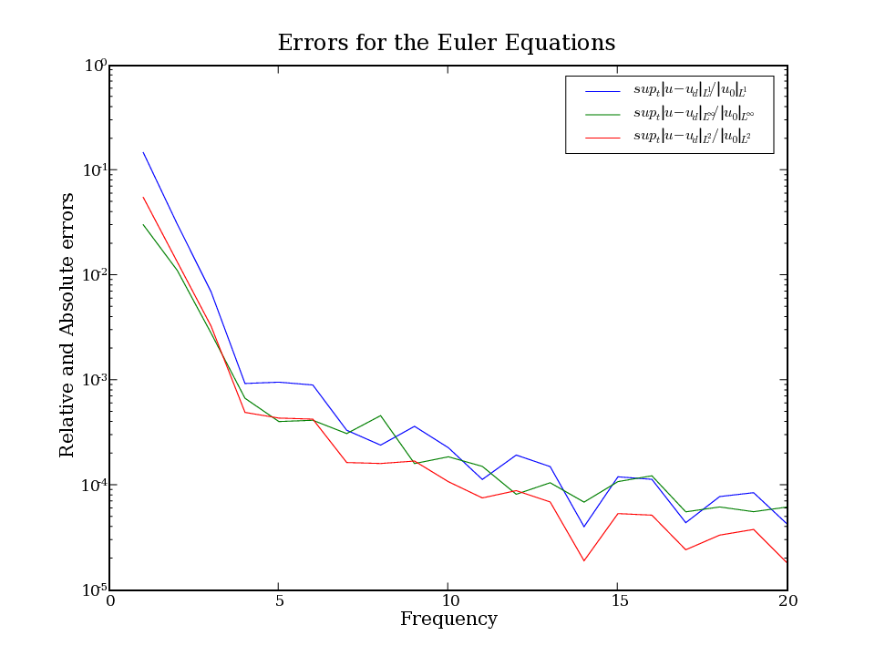
We solved the Euler equations on the region $[-32,32]^{2}$ with lattice spacing $\delta x=0.125$ (for a total of $512^{2}$ lattice points). Such a setup is valid for spatial frequencies up to $k_{\operatorname{max}}=\pi/\delta x=25.1$. We solved the system using the Fast Fourier transform to compute (1.3), which is accurate to machine precision provided no waves reach the boundary ([22, Theorem 4.1] or [21, Theorem A.1]). This accuracy is independent of time-step, which we took to be $\delta t=0.25$ in order to get a watchable frame-rate in the plots. The phase space filter region was taken to have width $16$ ($128$ lattice points), with $T_{\operatorname{step}}=1.5$, and $\sigma=1.0$. The initial condition was taken to be

with the $K$ varying from $1$ to $20$ (the frequency range of the problem). This yields an initial condition with frequency localized near $|\vec{k}|=K$. The results were compared to another simulation on a large box. The result is that for $K>4$, $L^{2}$ error of $10^{-3}$ (relative to the initial condition) is achieved up to $t=50$ (see Figure 3). The error at low frequencies can be dealt with by various means, see Section 4 and [21].

Let $\vec{E}$ be the electric field and $\vec{H}=\mu\vec{B}$ with $\vec{B}$ the magnetic field. Let $\epsilon$ and $\mu$ be the electrical and magnetic permeability’s of a medium.

In order to bring Maxwell’s equations to symmetric form, we introduce the auxiliary variable ${\vec{u}}=(\sqrt{\mu}\vec{H},\sqrt{\epsilon}\vec{E})^{T}$. With this formulation, the Hamiltonian for Maxwell’s equations can be written in block form:

where $\nabla\times$ is interpreted as a matrix,

The symmetry of $\epsilon$, $\mu$ and $\nabla\times$ implies that ${\mathcal{H}}$ is skew-adjoint.

To further simplify the system, we make the following additional assumptions. We assume $\mu=1$. We assume the system is $z$-independent, i.e. $\partial_{z}=0$, and we can restrict ourselves to two-dimensional simulations. Lastly, we simplify the electrical permittivity:

This is the simplest possible birefringent system. With the variables

we can write the dispersion relation as:

with

with $E(\vec{k})=\sqrt{(f^{2}+g^{2})(k_{1}^{2}+k_{2}^{2})-4fgk_{1}k_{2}}$.

This can be further simplified by noting that $u_{1},u_{2}$ and $u_{6}$ (corresponding to $B_{x},B_{y},E_{z}$ are uncoupled to $u_{3},u_{4}$ and $u_{5}$. The $u_{1},u_{2}$ and $u_{6}$ modes (corresponding to $B_{x},B_{y}$ and $E_{z}$) are actually isotropic waves, so we will ignore them. We therefore restrict consideration to $u_{3},u_{4}$ and $u_{5}$ ($u_{3}$ corresponds to $B_{z}$, and $u_{4,5}$ correspond to to linear combinations of $E_{x}$ and $E_{y}$).

We solved the reduced system of Maxwell’s equations with the same parameters as in Section 3.2, with the same initial condition (replacing $u_{1}$ by $u_{3}$ in (3.3a)). The anisotropy parameter $b$ was chosen to be $0.25$. The results are comparable to those for the Euler equation, see Figures 4 and 5.

In Theorem 1 of Section 2.3, it was proved that the phase space filtering algorithm is stable. To demonstrate the validity of the theorem, we ran a simulation of the Euler equations and Maxwell’s equations up to time $t=2000$. While we can not determine the accuracy over such long time intervals (the reference simulation would require an extremely large box), we can study the growth of the $L^{2}$-norm.

The results of such a simulation are plotted in Figure 6. They indicate that Theorem 1 is correct, and that the mass of the solution decreases monotonically with time.

References

- [1] Bradley Alpert, Leslie Greengard, and Thomas Hagstrom. Nonreflecting boundary conditions for the time-dependent wave equation. J. Comput. Phys., 180(1):270–296, 2002.
- [2] Alvin Bayliss and Eli Turkel. Radiation boundary conditions for wave-like equations. Comm. Pure Appl. Math., 33(6):707–725, 1980.
- [3] E. Becache, S. Fauqueux, and P. Joly. Stability of perfectly matched layers, group velocities and anisotropic waves. J. Comput. Phys., 188(1):399–433, 2003.
- [4] Jean-Pierre Berenger. A perfectly matched layer for the absorption of electromagnetic waves. J. Comput. Phys., 114(2):185–200, 1994.
- [5] Jean-Pierre Berenger. Three-dimensional perfectly matched layer for the absorption of electromagnetic waves. J. Comput. Phys., 127(2):363–379, 1996.
- [6] Emmanuel J. Candès and Laurent Demanet. The curvelet representation of wave propagators is optimally sparse. Comm. Pure Appl. Math., 58(11):1472–1528, 2005.
- [7] Ingrid Daubechies. Time-frequency localization operators: a geometric phase space approach. IEEE Trans. Inform. Theory, 34(4):605–612, 1988.
- [8] Björn Engquist and Andrew Majda. Absorbing boundary conditions for numerical simulation of waves. Proc. Nat. Acad. Sci. U.S.A., 74(5):1765–1766, 1977.
- [9] Bjorn Engquist and Andrew Majda. Absorbing boundary conditions for the numerical simulation of waves. Math. Comp., 31(139):629–651, 1977.
- [10] Björn Engquist and Andrew Majda. Radiation boundary conditions for acoustic and elastic wave calculations. Comm. Pure Appl. Math., 32(3):314–358, 1979.
- [11] Sandro Graffi and Kenji Yajima. Exterior complex scaling and the ac-stark effect in a coulomb field. Commun. Math. Phys., 89:277–301, 1983.
- [12] Thomas Hagstrom. Radiation boundary conditions for the numerical simulation of waves. In Acta numerica, 1999, volume 8 of Acta Numer., pages 47–106. Cambridge Univ. Press, Cambridge, 1999.
- [13] Thomas Hagstrom. New results on absorbing layers and radiation boundary conditions. In Topics in computational wave propagation, volume 31 of Lect. Notes Comput. Sci. Eng., pages 1–42. Springer, Berlin, 2003.
- [14] F.Q. Hu. On absorbing boundary conditions for linearized euler equations by a perfectly matched layer. J. Comput. Phys., 129:201–219, 1996.
- [15] Shidong Jiang and L. Greengard. Efficient representation of nonreflecting boundary conditions for the time-dependent schrodinger equation in two dimensions. Communications in Pure and Applied Mathematics, 61(2):261–288, 2008, http://web.njit.edu/ jiang/Papers/Schrodinger2d.pdf.
- [16] I. M. Navon, B. Neta, and M. Y. Hussaini. A perfectly matched layer approach to the linearized shallow water equations models. Monthly Weather Review, 132:1369–1378, 2004.
- [17] I. M. Sigal and A. Soffer. Asymptotic completeness of short-range many-body systems. Bull. Amer. Math. Soc. (N.S.), 14(1):107–110, 1986.
- [18] I. M. Sigal and A. Soffer. The -particle scattering problem: asymptotic completeness for short-range systems. Ann. of Math. (2), 126(1):35–108, 1987.
- [19] I. M. Sigal and A. Soffer. Asymptotic completeness of -particle long-range scattering. J. Amer. Math. Soc., 7(2):307–334, 1994.
- [20] Barry Simon. Resonances and complex scaling: A rigorous overview. Int. J. Quantum Chemistry, pages 529––542, 1978.
- [21] A. Soffer and C. Stucchio. Multiscale resolution of shortwave-longwave interactions in time dependent dispersive waves. Communications in Pure and Applied Mathematics, Accepted, arxiv.org/abs/0705.3501.
- [22] A. Soffer and C. Stucchio. Time dependent phase space filters: Nonreflecting boundaries for semilinear schrodinger equations. 2006. in preparation.
- [23] A. Soffer and C. Stucchio. Open boundaries for the nonlinear schrodinger equation. Journal of Computational Physics, 225(2):1218–1232, 2007, arxiv.org/abs/math/0609183.