An Information-Geometric Reconstruction of Quantum Theory, II:
The Correspondence Rules of Quantum Theory

Philip Goyal Email: pgoyal@perimeterinstitute.ca Affiliation: Perimeter Institute
Waterloo, Canada

Abstract

In a companion paper (hereafter referred to as Paper I), we have presented an attempt to derive the finite-dimensional abstract quantum formalism within the framework of information geometry. In this paper, we formulate a correspondence principle, the Average-Value Correspondence Principle, that allows relations between measurement results which are known to hold in a classical model of a system to be systematically taken over into the quantum model of the system. Using this principle, we derive the explicit form of the temporal evolution operator (thereby completing the derivation of the abstract quantum formalism begun in Paper I), and derive many of the correspondence rules (such as operator rules, commutation relations, and Dirac’s Poisson bracket rule) that are needed to apply the abstract quantum formalism to model particular physical systems.

pacs

03.65.-w, 03.65.Ta, 03.67.-a

I Introduction

In order to obtain a quantum mechanical model for a particular physical system such as a particle moving in space, it is necessary to supplement the abstract quantum formalism with various rules, to which we shall refer collectively as correspondence rules, which explicitly determine the form of the operators that represent particular measurements performed on the system, or that represent particular symmetry transformations (such as displacement or rotation) of the frame of reference in which the system is being observed. These correspondence rules can be usefully classified as follows:

(i)

Operator Rules. Rules for writing down operators representing measurements of observables that, in the framework of classical physics, are known functions of other, elementary, observables whose operators are given ¹¹ 1 The basic operator rules of quantum theory are (i) Rule 1 (Function rule): If $A\rightarrow\textsf{A}$ , then $f(A)\rightarrow f(\textsf{A})$ ; (ii) Rule 2 (Sum rule): If $A\rightarrow\textsf{A}$ and $B\rightarrow\textsf{B}$ , then $f_{1}(A)+f_{2}(B)\rightarrow f_{1}(\textsf{A})+f_{2}(\textsf{B})$ (and similarly for more than two observables), and (iii) Rule 3 (Product rule): If $A\rightarrow\textsf{A}$ and $B\rightarrow\textsf{B}$ , where $[\textsf{A},\textsf{B}]=0$ , then $f_{1}(A)f_{2}(B)\rightarrow f_{1}(\textsf{A})f_{2}(\textsf{B})$ (and similarly for more than two observables). A more general rule that is often employed is: (iv) Rule 3^′ (Hermitization rule): If $A\rightarrow\textsf{A}$ and $B\rightarrow\textsf{B}$ , then $f_{1}(A)f_{2}(B)\rightarrow(f_{1}(\textsf{A})f_{2}(\textsf{B})+f_{2}(\textsf{B})f_{1}(\textsf{A}))/2$ .. For example, such rules are needed to be able to write down the operator that represents a measurement of $H$ , given the classical relation $H=p_{x}^{2}/2m+V(x)$ , in terms of the operators x and $\textsf{p}_{x}$ which represent measurements of $x$ and $p_{x}$ , respectively.
(ii)

Measurement Commutation Relations. Commutation relations between operators that represent measurements of fundamental observables such as position, momentum, and components of angular momentum. The commutation relations $[\textsf{x},\textsf{p}_{x}]=i\hbar$ and $[\textsf{L}_{x},\textsf{L}_{y}]=i\hbar\textsf{L}_{z}$ , are the obvious examples, while Dirac’s Poisson bracket rule, $[\textsf{A},\textsf{B}]=i\hbar\widehat{\{A,B\}}$ , is the more general rule, where $\{A,B\}$ is the classical Poisson bracket for observables $A$ and $B$ , and $\widehat{\{A,B\}}$ , A, and B are the respective operators.
(iii)

Measurement–Transformation Commutation Relations. The commutation relations between measurement operators and transformation operators. For example, in the case of the $x$ -displacement operator, $\textsf{D}_{x}$ , one has, for example, $[\textsf{x},\textsf{D}_{x}]=i$ and $[\textsf{p}_{x},\textsf{D}_{x}]=0$ .
(iv)

Transformation Operators. Explicit forms of the operators that represent symmetry transformations of a frame of reference, such as the $x$ -displacement operator $\textsf{D}_{x}=-i\,d/dx$ .

The physical origin of many of the above-mentioned rules is obscure. For example, although one can give simple physical arguments ²² 2 See [11] (Sec. 11) and [5] (Sec. IV.1), for example. for the operator rule which states that, if a measurement of $A$ is represented by operator A, then a measurement of the function $f(A)$ is represented by operator $f(\textsf{A})$ , the generalization of such arguments to measurements of functions of two or more observables encounters severe difficulties due to the possible non-commutativity of the operators that represent these observables. As a result of such difficulties, operator rules tend to be heuristic and tend to lead to inconsistencies when applied to particular examples ³³ 3 See, for example, [5] (Sec. IV.1), [12] (Sec. 9.12—9.15), and [13] (Sec. 5.2.1). We shall discuss one such example in Sec. III.1.. Similarly, the commutation relationship $[\textsf{x},\textsf{p}_{x}]=i\hbar$ is typically obtained from Schroedinger’s equation or from Dirac’s Poisson bracket rule, both of whose derivations involve abstract assumptions whose physical origin is obscure.

The question of what additional physical ideas are needed to obtain the correspondence rules described above given the abstract quantum formalism has received relatively little recent attention. Recent work on the elucidation of the physical origin of the quantum formalism (see Paper I for references [1]) tends to neglect the question of the physical origin of the correspondence rules or is concerned with the derivation of the Schroedinger equation directly from physical ideas without taking the abstract quantum formalism as a given [2, 3, 4].

Operator rules have been discussed in a few publications, for example in [5, 6], but a derivation of the operator rules on the basis of a physical principle, taking the abstract formalism as a given, has not been successfully completed. The most recent systematic attempt to derive the commonly employed measurement and measurement–transformation commutation relations in such a manner is found in [7] (see also Refs. [8, 9]). In [7], using the commutation relationships for the operators that represent the Galilean group of transformations, and establishing the relation between these transformation operators and particular measurement operators, commutation relations for these measurement operators are obtained. However, this approach implicitly makes use of operator rules, and relies upon auxiliary assumptions (such as the assumption that certain measurement operators are unchanged by the action of particular symmetry operators) whose physical origin is unclear.

In this paper, we show that, starting from the abstract quantum formalism, it is possible to derive all the above-mentioned correspondence rules in a systematic manner from a single correspondence principle. The principle, called the Average-value Correspondence Principle (AVCP), rests on the simple, intuitive notion that the quantum and classical models of the same physical system (such as a particle moving in a potential) should agree in their predictions if one compares the expected values of the quantum measurements with the values obtained from the corresponding classical measurements, a connection which is known, via Ehrenfest’s theorem, to hold approximately between the classical and quantum models of a particle [10].

The principle expresses the classical-quantum correspondence in the following form: in a classical experiment, if a measurement of observable $A$ on a physical system can be implemented by an arrangement where measurements of observables $A^{\prime},A^{\prime\prime},\dots$ are performed on the system (possibly performed at a different time to the measurement of $A$ ), such that the value obtained from measurement of $A$ can be calculated as a function, $f$ , of the values obtained from the measurements of $A^{\prime},A^{\prime\prime},\dots$ , then we can construct a corresponding quantum experiment, where quantum measurements $\mathbf{A},\mathbf{A}^{\prime},\mathbf{A}^{\prime\prime},\dots$ , corresponding to classical measurements of $A,A^{\prime},A^{\prime\prime},\dots$ , are performed on copies of the same physical system, such that the same functional relation holds on average between the values obtained from the quantum measurements, where the average is taken over infinitely many trials of the quantum experiment. This connection holds only if $f$ satisfies a particular condition. The particular form of the quantum experiment is stipulated by the AVCP, and consists in specifying whether, for each pair of quantum measurements, the measurements in the pair are performed on the same or different copies of the system.

This paper is organized as follows. We begin in Sec. II by formulating the AVCP. In Sec. III, the AVCP is used to obtain several generalized operator rules which connect the average values of operators at different times, from which the commonly used operator rules of quantum theory follow as a special case. Using the AVCP and the Temporal Evolution postulate (from Paper I), we then derive the explicit form of the temporal evolution operator, thereby completing the derivation of the finite-dimensional abstract quantum formalism begun in Paper I.

Next, in Sec. IV, taking the infinite-dimensional form of the abstract quantum formalism as a given, we use the AVCP to derive many of the commonly employed correspondence rules of quantum theory, namely (a) the commutation relations $[\textsf{x},\textsf{p}_{x}]=i\hbar$ and $[\textsf{L}_{x},\textsf{L}_{y}]=i\hbar\textsf{L}_{z}$ , and Dirac’s Poisson bracket rule, (b) the explicit form of the operators for displacements and rotations, and (c) the commutation relations between momentum and displacement operators, and between angular momentum and rotation operators.

We note that the treatment of the correspondence rules is illustrative rather than exhaustive, so that only the most commonly encountered measurement and transformation operators which are needed to formulate non-relativistic and relativistic quantum mechanics have been discussed. Many other correspondence rules (such as the operators that represent Galilei transformations, temporal displacement, and discrete transformations such as spatial inversion) can be obtained by arguments which closely follow those presented. The paper concludes with a discussion of the results obtained.

II The Average-Value Correspondence Principle

II.1 Introduction

Suppose that, as described in Paper I, a quantum model $\mathbf{q}(N)$ , of dimension $N$ , has been constructed to describe an abstract experimental set-up consisting of a source of identical systems, a measurement set $\mathcal{A}$ , and an interaction set $\mathcal{I}$ . The measurements in $\mathcal{A}$ , and the degenerate forms of measurements in $\mathcal{A}$ ⁴⁴ 4 A measurement that is a degenerate form of a measurement $\mathbf{A}$ is defined operationally in Paper I. Such a measurement has $N^{\prime}<N$ possible results, and can be represented as an $N$ -dimensional degenerate Hermitian operator (with $N^{\prime}$ distinct eigenvalues)., are represented by $N$ -dimensional Hermitian operators (possibly with degenerate eigenvalues), and shall be called quantum measurements.

Suppose that quantum measurement $\mathbf{A}$ , with operator A, represents a measurement that is classically described as a measurement of some observable $A$ (which we shall henceforth abbreviate to “quantum measurement $\mathbf{A}$ (or operator A) represents a (classical) measurement of $A$ ”). Suppose that we wish to determine whether there is a quantum measurement that represents a measurement of, say, $A^{2}$ , and, if so, to determine the operator which can be said to represent this measurement. Classically, one can imagine that a measurement of $A^{2}$ is implemented by an experimental arrangement where a measurement of $A$ is performed and the value obtained is then squared. If this arrangement is described in the quantum model, it follows that, if the input state is an element, $\textsf{v}_{i}$ , of an orthonormal set of eigenvectors of A, the output state of the process is $\textsf{v}_{i}$ and the output of the process is $a_{i}^{2}$ , where $\textsf{A}\textsf{v}_{i}=a_{i}\textsf{v}_{i}$ ( $i=1,2,\dots,N$ ). According to this line of reasoning, it follows at once that the operator $\sum_{i}a_{i}^{2}\textsf{v}_{i}^{\dagger}\textsf{v}_{i}=\textsf{A}^{2}$ therefore represents a measurement of $A^{2}$ .

However, this simple argument, given by Dirac [11], does not readily generalize. For example, suppose that quantum measurements $\mathbf{A}$ and $\mathbf{B}$ , with operators A and B, represent measurements of $A$ and $B$ , respectively. Suppose that we wish to determine the operator (if any exists) that represents a measurement of $A+B$ . Classically, one imagines that such a measurement is implemented by making measurements of $A$ and $B$ simultaneously on a system, and adding the values obtained. However, if $[\textsf{A},\textsf{B}]\neq 0$ , this arrangement cannot be described in the quantum framework since, in this framework, the measurements cannot be performed at the same time on a single system. If one, then, instead considers an arrangement where, for instance, a measurement of $A$ is followed immediately by a measurement of $B$ , then, if the arrangement is described in the quantum framework, one cannot find $N$ input states which emerge as output states since the non-commutativity of A and B implies that A and B share fewer than $N$ eigenstates in common, making it impossible to construct a simple parallel to Dirac’s argument.

Now, the conventional operator rules of quantum theory assert that a measurement of $A+B$ is represented by the operator $\textsf{A}+\textsf{B}$ . Although this seems entirely reasonable on a formal, symbolic level, it is not clear in what physical sense $\textsf{A}+\textsf{B}$ can be said to ‘represent’ the measurement. To see this, note that, whereas the eigenvectors and eigenvalues of A directly reflect the output states and the values obtained when measurement $\mathbf{A}$ is performed on the system, the eigenvectors of $\textsf{A}+\textsf{B}$ do not, in general, coincide with the eigenvectors of either A or B, and the eigenvalues of $\textsf{A}+\textsf{B}$ do not, in general, coincide with the outputs of any plausible arrangement (described in the quantum model) that classically implements a measurement of $A+B$ which involves performing measurements of $A$ and $B$ and combining the values obtained. For example, a classical measurement of $S_{x}+S_{z}$ is implemented by an arrangement where measurements of $S_{x}$ and $S_{z}$ are performed immediately after one another, and their values added. When modeled in the quantum framework, the possible outputs of this arrangement, in the case where the measurements are performed on a spin-1/2 particle, are $\pm\hbar,0$ , whereas a quantum measurement represented by operator $\textsf{S}_{x}+\textsf{S}_{z}$ has possible values $\pm\hbar/\sqrt{2}$ .

The above observations illustrate the difficulty of obtaining a physical understanding of the operator rules of quantum theory even in simple cases of interest. Below, we shall formulate a physical principle which gives a clear physical meaning to the sense in which an operator can be said to represent a classical measurement, and, in the majority of cases of interest, uniquely determines the operator which represents such a measurement.

II.1.1 Implementations of classical measurements

Consider again a measurement of $A^{2}$ , where $A$ is some observable. Classically, one can imagine a measurement of $A^{2}$ being implemented using one of three different arrangements (see Fig. 1): (i) make a measurement of $A$ on one copy of the system, and square the value obtained; (ii) make two immediately successive measurements of $A$ on one copy of the system, and multiply the two values obtained; or (iii) make two simultaneous measurements of $A$ on two separate copies of the system prepared in the same state, and multiply the two values obtained. Although the first of these arrangements is the one we have considered above, all three arrangements yield the same output when modeled classically, and so can be regarded as equally valid implementations of a measurement of $A^{2}$ in the classical framework.

Refer to caption — Figure 1: Three arrangement that classically implement a measurement of $A^{2}$ . In (i), a measurement of $A$ is made on one copy of the system, and the value obtained is squared to give the output; in (ii), two immediately successive measurements of $A$ are made on one copy of the system, and the output is obtained by multiplying the two values obtained; and (iii) two simultaneous measurements of $A$ are made on two separate copies of the system prepared in the same state, and the output is obtained by multiplying the two values obtained. In a classical model of these arrangements, each arrangement yields the same output. However, in the quantum model of these arrangements, the expected output of (i) and (ii) is $\overline{a^{2}}$ whereas the expected output of (iii) is $(\overline{a})^{2}$ .

Now, perhaps surprisingly, when described using the quantum model, these arrangements do not, in general, yield the same expected outputs. Consider a quantum theoretic description of the first arrangement where quantum measurement $\mathbf{A}$ represents a measurement of $A$ . In each run of the experiment, one copy of the system is prepared in some given state. Let the probability that a measurement $\mathbf{A}$ yields result $i$ ( $i=1,2,\dots,N$ ), with value $a_{i}$ , be denoted $p_{i}$ . Then, the expected output is given by

\begin{split}\text{Expected output}&=\sum_{i}(a_{i})^{2}p_{i}\\ &=\overline{a^{2}}\end{split}

(1)

One finds that arrangement (ii) yields the same expected output. However, in arrangement (iii), where, in each run of the experiment, two copies of the system are prepared in the same state, one obtains

\begin{split}\text{Expected output}&=\sum_{i,j}(a_{i}a_{j})p_{i}p^{\prime}_{j}\\ &=(\overline{a})^{2},\end{split}

(2)

with $p_{i}$ and $p^{\prime}_{j}$ denoting respectively the probabilities that measurements $\mathbf{A}$ on the first and second copy yield result $i$ and $j$ ( $i,j=1,2,\dots,N$ ).

In this example, the differences between the arrangements as viewed in the quantum model arise due to the fact that, in the quantum framework, an immediate repetition of a measurement on the same copy of a system is different from performing a second simultaneous measurement on a separate, identically-prepared, copy of the system.

In the case of a measurement of $A+B$ , where measurements of $A$ and $B$ are assumed to occur at the same time, one needs to take into account the additional fact that, in the quantum framework, the order in which two measurements is performed is of possible importance. Accordingly, one can imagine implementing a measurement of $A+B$ using one of at least three arrangements (see Fig. 2): (i) make a measurement of $A$ , and then a measurement of $B$ , on one copy of the system, and add the values obtained; (ii) make a measurement of $B$ , and then a measurement of $A$ , on one copy of the system, and add the values obtained; (iii) make a measurement of $A$ on one copy of the system and, simultaneously, a measurement of $B$ on a second copy of the system prepared in the same state as the first copy, and add the values obtained. Once again, in a classical model of these arrangements, the outputs agree. However, if one calculates the expected outputs in the quantum model, one finds that, if $[\textsf{A},\textsf{B}]\neq 0$ , all three will, in general, disagree with one another.

As these examples illustrate, different arrangements that implement the same classical measurement do not, in general, give the same expected output when described in the quantum framework.

II.1.2 The average-value condition

The existence of different arrangements that implement the same classical measurement immediately raises two questions. First, are these arrangements, in some sense, equally valid in the quantum framework, or it is possible to find some reasonable physical basis upon which to select particular arrangements and regard these as more fundamental than the others? Second, is it possible to find operators that represent the selected arrangements, and, if so, do all the selected arrangements that implement a given measurement have the same operator representation?

To answer these questions, we begin by observing that, although the above arrangements are all regarded as bone fide implementations of measurements in the classical model, a measurement is only describable as such in the quantum model, and so can be called a quantum measurement, if it can be represented by a Hermitian operator which represents a single measurement performed upon one copy of the system at a particular time. So, for example, although arrangement (iii) of a measurement of $A^{2}$ can be modeled in the quantum framework, it cannot be described as a quantum measurement since it involves two separate measurements. In contrast, arrangement (i) can be described as a quantum measurement since it only involves a single measurement on one copy of the system.

However, although an arrangement involving more than one measurement cannot itself be regarded as a quantum measurement when modeled in the quantum framework, we can reasonably ask whether it is possible to find a quantum measurement, $\mathbf{C}$ , with operator C, which, in some sense to be determined, can nonetheless be said to represent the arrangement.

At the outset, we note that it makes no sense to require that measurement $\mathbf{C}$ always yield a value that coincides with the output of a given arrangement since measurement results are only probabilistically determined in the quantum framework. However, we can impose the simple condition that, over an infinite number of runs, the average value obtained from measurement $\mathbf{C}$ should coincide with the average output obtained from the arrangement for any initial state of the system.

For example, in the case of an arrangement that implements a measurement of $A^{2}$ , quantum measurement $\mathbf{C}$ which, by hypothesis, represents the arrangement, must be such that, for all states of the system, $\langle\textsf{C}\rangle$ is equal to the expected output obtained from the arrangement. In the case of arrangements (i) and (ii) described above, using Eq. (1), we accordingly obtain the condition that the relation

\begin{split}\langle\textsf{C}\rangle&=\overline{a^{2}}\\ &=\langle\textsf{A}^{2}\rangle\end{split}

(3)

must hold for all states, v, of the system. From this condition, we can conclude that

\textsf{C}=\textsf{A}^{2}.

(4)

In the case of arrangement (iii), using Eq. (2), we obtain the condition that the relation

\begin{split}\langle\textsf{C}\rangle&=(\overline{a})^{2}\\ &=\langle\textsf{A}\rangle^{2}\end{split}

(5)

must hold for all v. By diagonalizing A, one can readily show that this condition implies that A is a multiple of the identity, which represents a trivial measurement that yields the same result irrespective of the state of the system. Therefore, arrangement (iii) does not satisfy the above average-value condition in the case of any non-trivial measurement of $A$ , and can therefore be reasonably eliminated. Hence, in this case, the average-value condition is sufficiently strong so as to be able to pick out arrangements (i) and (ii), and, since the average-value condition also implies that these arrangements are both represented by the operator, $\textsf{A}^{2}$ , one can unambiguously conclude that a measurement of $A^{2}$ is represented by the operator $\textsf{A}^{2}$ .

Proceeding in a similar way, restricting ourselves for the time being to measurements $\mathbf{A}$ and $\mathbf{B}$ that are not subsystem measurements ⁵⁵ 5 A subsystem measurement is defined in Paper I as a measurement performed on a single subsystem of a composite system., one finds that, in the case of a measurement of $C=A+B$ , only arrangement (iii) is possible if $[\textsf{A},\textsf{B}]\neq 0$ , which then yields the operator

\textsf{C}=\textsf{A}+\textsf{B}.

(6)

If $[\textsf{A},\textsf{B}]=0$ , then all three arrangements are possible, and all yield the same operator, C, as above.

Finally, in the case of a measurement of $AB$ , with $[\textsf{A},\textsf{B}]=0$ , one finds that the arrangement must be the one where measurements $\mathbf{A}$ and $\mathbf{B}$ are performed on the same copy of the system, in which case the operator AB is obtained.

Hence, we see that the average-value condition is sufficient to yield a unique operator representation for the measurements considered above. Based on the above considerations, we can tentatively formulate the following general rule: in the case of a measurement which is implemented by an arrangement that contains two elementary measurements (not subsystem measurements) represented by commuting operators, it is possible to find a quantum measurement that represents the arrangement if the two elementary measurements are performed on the same copy of the system; but, when the operators do not commute, the elementary measurements must be performed on different copies of the system.

We now consider implementations of a measurement of $AB$ in the case when $[\textsf{A},\textsf{B}]\neq 0$ . The general rule just given suggests that we should consider the arrangement where the measurements of $A$ and $B$ are performed on different copies of the system. When described in the quantum framework, this arrangement has the expected output

\sum_{i}\sum_{j}(a_{i}b_{j})p_{i}p_{j}^{\prime}=\langle\textsf{A}\rangle\langle\textsf{B}\rangle,

(7)

with $p_{i}$ and $p^{\prime}_{j}$ denoting respectively the probabilities that the measurement $\mathbf{A}$ on the first copy and the measurement $\mathbf{B}$ on the second copy yield result $i$ and $j$ ( $i,j=1,2,\dots,N$ ), and $a_{i},b_{j}$ respectively denoting the values of the $i$ th and $j$ th results of measurements $\mathbf{A}$ and $\mathbf{B}$ . Imposing the above average-value condition, the operator C that represents this implementation must satisfy the condition

\langle\textsf{C}\rangle=\langle\textsf{A}\rangle\langle\textsf{B}\rangle

(8)

for all v. However, for non-commuting A and B, one finds that C cannot be found such that this relation is satisfied for all v. We note, however, that with

\textsf{C}=\frac{1}{2}(\textsf{A}\textsf{B}+\textsf{B}\textsf{A}),

(9)

equation (8) holds for the eigenstates of A and the eigenstates of B, which suggests that we may be able to weaken the average-value condition in this case so that we only require that Eq. (8) holds for these eigenstates. However, as we shall illustrate later (Sec. III.1), the application of Eq. (9) can lead to inconsistencies. Consequently, we conclude that, from the point of view of the average-value condition, it is not possible to find an operator that represents a measurement of $AB$ when the operators A and B do not commute. More generally, we find that, when $[\textsf{A},\textsf{B}]\neq 0$ , it is necessary to exclude measurements of $f(A,B)$ , with $f$ analytic (so that $f$ has a well-defined polynomial expansion in $A$ and $B$ ), where the polynomial expansion of $f$ contains product terms.

Finally, in the case of a classical measurement which is implemented by an arrangement which contains two measurements that are performed on different subsystems of a composite system, one finds that the arrangement can be represented by a quantum measurement irrespective of whether the two measurements are performed on the same or on different copies of the system, and that the different possible arrangements are represented by the same operator.

II.1.3 Generalizations

In the examples above, we have considered arrangements that implement a classical measurement in which the measurement and the measurements in the arrangement are performed at the same time, and in the same frame of reference. However, as the following examples illustrate, these are unnecessary restrictions.

First, classically, for a non-relativistic particle of mass $m$ , one can implement a measurement of $x$ performed at time $t+\delta t$ by an arrangement where measurements of $x$ and $p_{x}$ are performed at time $t$ , and the function $x+p_{x}\,\delta t/m$ is then computed.

Second, one can implement a measurement of $x^{\prime}$ on a particle in the reference frame $S^{\prime}$ that is displaced along the $x$ -axis relative to frame $S$ by performing a measurement of $x$ in frame $S$ , and computing the appropriate function $x^{\prime}=f(x)$ that relates $x$ and $x^{\prime}$ .

The above considerations regarding the implementation of a classical measurement are applicable without change to the case where the measurement and the measurements in the arrangement by which it is implemented are performed at different times or in different frames of reference. Below, we shall accordingly generalize our notion of the implementation of a classical measurement.

II.2 Statement of the AVCP

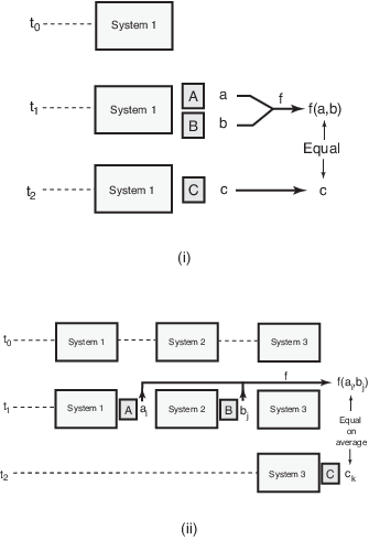
We shall now state a general principle which incorporates the observations made above concerning the average-value condition. An illustrative example is given in Fig. 3.

Average-Value Correspondence Principle Consider a classical idealized experiment in which a system (possibly a composite system) is prepared in some state at time $t_{0}$ , and is allowed to evolve in a given background. Suppose that a measurement of $A^{(m)}$ $(m\geq 2)$ , performed on the system at time $t_{2}$ with value $a^{(m)}$ , can be implemented by an arrangement where measurements of $A^{(1)},A^{(2)},\dots,A^{(m-1)}$ are performed upon one copy of the system at time $t_{1}$ , and the values of their respective results, denoted $a^{(1)},a^{(2)},\dots,a^{(m-1)}$ , are then used to compute the output $f(a^{(1)},a^{(2)},\dots,a^{(m-1)})$ , where $f$ is an analytic function, so that the relation

$a^{(m)}=f(a^{(1)},a^{(2)},\dots,a^{(m-1)})$ ( $*$ )

holds for all initial (classical) states of the system.

Consider the case where the quantum measurements $\mathbf{A}^{(1)},\mathbf{A}^{(2)},\dots,\mathbf{A}^{(m)}$ , with operators $\textsf{A}^{(1)},\textsf{A}^{(2)},\dots,\textsf{A}^{(m)}$ , represent the measurements of $A^{(1)},A^{(2)},\dots,A^{(m)}$ , respectively. Then, consider the following idealized quantum experimental arrangement consisting of several set-ups, each consisting of identical sources and backgrounds, where, in each set-up, a copy of the system is prepared in the same initial state, $\textsf{v}_{0}$ , at time $t_{0}$ .
In one set-up, only measurement $\mathbf{A}^{(m)}$ is performed (at time $t_{2}$ ) and, for any $i,j$ with $i\neq j$ and $i,j\leq m-1$ , the measurements $\mathbf{A}^{(i)},\mathbf{A}^{(j)}$ are performed (at time $t_{1}$ ) in:
1. 1.
  
  the same set-up if both $\bigl[\textsf{A}^{(i)},\textsf{A}^{(j)}\bigr]=0$ and, if the system is composite, the measurements are performed on the same subsystem;
2. 2.
  
  different set-ups if $\bigl[\textsf{A}^{(i)},\textsf{A}^{(j)}\bigr]\neq 0$ .
Let the values of the results of the measurements $\mathbf{A}^{(1)},\dots,\mathbf{A}^{(m)}$ in any given run of the experimental arrangement be denoted $a^{(1)},\dots,a^{(m)}$ , respectively. The function $f(a^{(1)},a^{(2)},\dots,a^{(m-1)})$ is defined as simple provided that its polynomial expansion contains no terms involving a product of eigenvalues belonging to measurements whose operators do not commute. If $f$ is simple, then ( ∗ ‣ II.2) holds on average, the average being taken over an infinitely large number of runs of the experiment.

The above principle can be generalized in a number of ways, for example to the case where the measurements of $A^{(1)},\dots,A^{(m-1)}$ are not performed at the same time. However, these generalizations are unnecessary for the derivations of the usual correspondence rules of quantum theory, and are therefore not discussed here.

III Generalized Operator Rules and the Temporal Evolution Operator

III.1 Generalized Operator Rules

We will now apply the AVCP to derive operator relations which hold when the function $f$ takes various useful forms. In each instance of $f$ , we shall first derive a generalized operator rule which relates the expected values of the relevant operators at different times. Then, taking the special case when the expected values are computed at the same time, we obtain the corresponding operator rule which relates the operators themselves.

We shall consider a classical experiment where a system is subject to measurements of $A$ and $B$ at time $t_{1}$ , and to a measurement of $C$ at time $t_{2}$ . We shall suppose that a measurement of $C$ , with value $c$ , can be implemented by an arrangement in which the measurements of $A$ and $B$ are performed, with respective values $a$ and $b$ , and the function $f(a,b)$ then computed, so that the relation

c=f(a,b)

(10)

holds for all initial states of the system.

In a quantum model of the appropriate experimental arrangement, let the operators that represent these measurements be denoted A, B, and C, respectively. To simplify the presentation, we shall only consider the case where these operators have finite dimension, $N$ ; the results obtained below can be readily shown to apply in the infinite dimensional case. Let the elements of orthonormal sets of eigenvectors of $\textsf{A},\textsf{B}$ and C be denoted $\textsf{v}_{i},\textsf{v}_{j}^{\prime}$ , and $\textsf{v}^{\prime\prime}_{k}$ , respectively $(i,j,k=1,2,\dots,N)$ , let the corresponding eigenvalues be denoted $a_{i},b_{j}$ and $c_{k}$ , and let the probabilities of the $i$ th, $j$ th and $k$ th results of measurements $\mathbf{A}$ , $\mathbf{B}$ and $\mathbf{C}$ in any given experimental arrangement be denoted by $p_{i}$ , $p^{\prime}_{j}$ and $p_{k}^{\prime\prime}$ , respectively.

Case 1. $f$ is a function of $a$ only.

In this case, the quantum experiment simply consists of two set-ups, involving two copies of the system, where $\mathbf{A}$ is performed on one copy at time $t_{1}$ and $\mathbf{C}$ on the other copy at time $t_{2}$ . Since function $f$ is simple, by the AVCP, the relation

\sum_{k}c_{k}p_{k}^{\prime\prime}=\sum_{i}f(a_{i})p_{i}

(11)

holds for all initial states, $\textsf{v}_{0}$ , of the system. Explicitly,

	$\displaystyle p_{i}$	$\displaystyle=\big\|\textsf{v}_{i}^{\dagger}\textsf{v}_{t_{1}}\big\|^{2}$		(12)
	$\displaystyle p_{k}^{\prime\prime}$	$\displaystyle=\big\|\textsf{v}_{k}^{\prime\prime\dagger}\textsf{v}_{t_{2}}\big\|^{2},$		(12)

with $\textsf{v}_{t}$ being the state of the relevant copy of the system at time $t$ . Hence, we can write Eq. (11) as

\textsf{v}^{\dagger}_{t_{2}}\bigg(\sum_{k}\textsf{v}_{k}^{\prime\prime}{\textsf{v}^{\prime\prime}_{k}}^{\dagger}c_{k}\bigg)\textsf{v}_{t_{2}}=\textsf{v}^{\dagger}_{t_{1}}\bigg(\sum_{i}\textsf{v}_{i}\textsf{v}_{i}^{\dagger}f(a_{i})\bigg)\textsf{v}_{t_{1}}.

(13)

Noting that

	$\displaystyle f(\textsf{A})$	$\displaystyle=\sum_{i}\textsf{v}_{i}\textsf{v}_{i}^{\dagger}f(a_{i})$		(14)
	$\displaystyle\textsf{C}$	$\displaystyle=\sum_{k}\textsf{v}_{k}^{\prime\prime}{\textsf{v}^{\prime\prime}_{k}}^{\dagger}c_{k},$		(14)

we obtain the relation

\langle\textsf{C}\rangle_{t_{2}}=\bigl\langle f(\textsf{A})\bigr\rangle_{t_{1}},

(15)

which holds for all $\textsf{v}_{0}$ . We can summarize the above result in the form of the generalized function rule:

c(t_{2})=f\left(a(t_{1})\right)\mapsto\langle\textsf{C}\rangle_{t_{2}}=\bigl\langle f(\textsf{A})\bigr\rangle_{t_{1}}\quad\forall\textsf{v}_{0},

(16)

where, for clarity, the times at which the results are obtained has been explicitly indicated. In the special case where $t=t_{1}=t_{2}$ , we obtain the usual operator rule, the function rule:

c=f(a)\mapsto\textsf{C}=f(\textsf{A}).

(17)

Case 2. $f(a,b)=f_{1}(a)+f_{2}(b)$

It is necessary to consider three sub-cases. First, if measurements $\mathbf{A}$ and $\mathbf{B}$ have commuting operators and, in the case of a composite system, if they are subsystem measurements performed on the same subsystem, then, by the AVCP, they are performed on the same copy of the system in the quantum experiment. Since $f$ is simple, the AVCP applies, so that

\begin{split}\sum_{k}c_{k}p_{k}^{\prime\prime}&=\sum_{i}\bigg(f_{1}(a_{i})+\sum_{j}f_{2}(b_{j})p^{\prime}_{j|i}\bigg)p_{i}\\ &=\sum_{i}\big(f_{1}(a_{i})+f_{2}(b_{i})\big)p_{i},\end{split}

(18)

holds for all initial states, $\textsf{v}_{0}$ , of the system. Here, the notation $p^{\prime}_{j|i}$ is the probability that measurement $\mathbf{B}$ yields result $j$ given that $\mathbf{A}$ has yielded result $i$ ; in this case, $p^{\prime}_{j|i}=\delta_{ij}$ . From the above relation, we obtain the generalized operator relation

\langle\textsf{C}\rangle_{t_{2}}=\bigl\langle f_{1}(\textsf{A})\bigr\rangle_{t_{1}}+\bigl\langle f_{2}(\textsf{B})\bigr\rangle_{t_{1}},

(19)

which holds for all initial states, $\textsf{v}_{0}$ . In the special case where $t_{1}=t_{2}$ , we obtain the operator relation,

\textsf{C}=f_{1}(\textsf{A})+f_{2}(\textsf{B}).

(20)

Second, in the case where measurements $\mathbf{A}$ and $\mathbf{B}$ are subsystem measurements performed on different subsystems, they can, by the AVCP, be performed on the same copy of the system, in which case we obtain the same results as above.

Third, if measurements $\mathbf{A}$ and $\mathbf{B}$ have non-commuting operators, then, by the AVCP, they are performed on different copies of the system in the quantum experiment. Since $f$ is simple, the AVCP again applies, so that the relation

\sum_{k}c_{k}p_{k}^{\prime\prime}=\sum_{i}f_{1}(a_{i})p_{i}+\sum_{j}f_{2}(b_{j})p_{j}^{\prime}

(21)

holds for all initial states of the system, which yields the same relation as in Eq. (19).

Hence, combining the foregoing three sub-cases, we obtain the generalized sum rule:

c(t_{2})=f_{1}\left(a(t_{1})\right)+f_{2}\left(b(t_{1})\right)\\ \mapsto\langle\textsf{C}\rangle_{t_{2}}=\bigl\langle f_{1}(\textsf{A})\bigr\rangle_{t_{1}}+\bigl\langle f_{2}(\textsf{B})\bigr\rangle_{t_{1}}\quad\forall\textsf{v}_{0}.

(22)

In the special case where $t=t_{1}=t_{2}$ , we obtain the sum rule:

c=f_{1}(a)+f_{2}(b)\mapsto\textsf{C}=f_{1}(\textsf{A})+f_{2}(\textsf{B}).

(23)

More generally, in the case of a classical experiment where measurements of $A^{(1)},A^{(2)},\dots,A^{(m-1)}$ are performed on a system at time $t_{1}$ and a measurement of $A^{(m)}$ at time $t_{2}$ , with values $a^{(1)},\dots,a^{(m)}$ , respectively, the AVCP implies the generalized operator rule:

a^{(m)}(t_{2})=\sum_{l=1}^{m-1}f_{l}\bigl(a^{(l)}(t_{1})\bigr)\\ \mapsto\bigl\langle\textsf{A}^{(m)}\bigr\rangle_{t_{2}}=\sum_{l=1}^{m-1}\bigl\langle f_{l}(\textsf{A}^{(l)})\bigr\rangle_{t_{1}}\quad\forall\textsf{v}_{0}.

(24)

Taking the special case of simultaneous measurements ( $t_{1}=t_{2}$ ), we obtain the operator rule

a^{(m)}=\sum_{l=1}^{m-1}f_{l}(a^{(l)})\mapsto\textsf{A}^{(m)}=\sum_{l=1}^{m-1}f_{l}(\textsf{A}^{(l)}).

(25)

Case 3. $f(a,b)=f_{1}(a)f_{2}(b)$

We again consider three sub-cases. First, if measurements $\mathbf{A}$ and $\mathbf{B}$ are represented by commuting operators and, if the measurements are subsystem measurements and are performed on the same subsystem, then, in the quantum experiment, they are performed on the same copy of the system. Since $f$ is, therefore, simple, the AVCP applies, so that the relation

\begin{split}\sum_{k}c_{k}p_{k}^{\prime\prime}&=\sum_{i,j}f_{1}(a_{i})f_{2}(b_{j})p_{i}p^{\prime}_{j|i}\\ &=\sum_{i}f_{1}(a_{i})f_{2}(b_{i})p_{i}\end{split}

(26)

holds for all initial states, $\textsf{v}_{0}$ , of the system. Hence, the generalized operator relation

\langle\textsf{C}\rangle_{t_{2}}=\bigl\langle f_{1}(\textsf{A})f_{2}(\textsf{B})\bigr\rangle_{t_{1}}

(27)

holds for all $\textsf{v}_{0}$ . In the case where measurements $\mathbf{A}$ , $\mathbf{B}$ , and $\mathbf{C}$ are simultaneous, we obtain the operator relation

\textsf{C}=f_{1}(\textsf{A})f_{2}(\textsf{B}).

(28)

Second, if measurements $\mathbf{A}$ and $\mathbf{B}$ are represented by commuting operators and are subsystem measurements performed on different subsystems of a composite system, then they can be performed on the same copy of the system in the quantum experiment, in which case we obtain the same result as above.

Third, if measurements $\mathbf{A}$ and $\mathbf{B}$ are represented by non-commuting operators, then the function $f$ is not simple, and the AVCP does not apply.

We can combine the three foregoing sub-cases to obtain the generalized product rule:

c(t_{2})=f_{1}\bigl(a(t_{1})\bigr)f_{2}\bigl(b(t_{1})\bigr)\\ \mapsto\langle\textsf{C}\rangle_{t_{2}}=\bigl\langle f_{1}(\textsf{A})f_{2}(\textsf{B})\bigr\rangle_{t_{1}}\quad\forall\textsf{v}_{0}\quad\text{if}~[\textsf{A},\textsf{B}]=0.

(29)

In the special case where $t_{1}=t_{2}$ , we obtain the product rule:

c=f_{1}(a)f_{2}(b)\mapsto\textsf{C}=f_{1}(\textsf{A})f_{2}(\textsf{B})\quad\text{if}~[\textsf{A},\textsf{B}]=0.

(30)

Some comments on inconsistencies

As mentioned in Sec. II.1.2, if the average-value condition is weakened to allow a measurement of $AB$ to be represented by an operator in the case where $[\textsf{A},\textsf{B}]\neq 0$ , one is lead to a rule that is often stated, namely

f_{1}(a)f_{2}(b)\mapsto\frac{1}{2}\bigl(f_{1}(\textsf{A})f_{2}(\textsf{B})+f_{1}(\textsf{A})f_{2}(\textsf{B})\bigr)

(31)

However, using this rule, one finds that inconsistencies quickly arise. For example, one can first apply this rule to find that the operator representing a measurement of $AB$ is

\widehat{AB}=(\textsf{A}\textsf{B}+\textsf{B}\textsf{A})/2,

(32)

where the notation $\widehat{X}$ is used to denote the operator that represents a measurement of $X$ . One can then apply the rule a second time to find the operator that represents a measurement of $A^{2}B$ . By treating this measurement as a measurement of $A(AB)$ , or as a measurement of $(A^{2})B$ , one obtains, respectively, either

\begin{split}\widehat{A(AB)}&=\frac{1}{2}(\textsf{A}\widehat{AB}+\widehat{AB}\textsf{A})\\ &=\frac{1}{4}\left(\textsf{A}(\textsf{A}\textsf{B}+\textsf{B}\textsf{A})+(\textsf{A}\textsf{B}+\textsf{B}\textsf{A})\textsf{A}\right)\\ &=\frac{1}{4}\left(\textsf{A}^{2}\textsf{B}+2\textsf{A}\textsf{B}\textsf{A}+\textsf{B}\textsf{A}^{2}\right),\end{split}

(33)

\begin{split}\widehat{(A^{2})B}&=\frac{1}{2}(\widehat{A^{2}}\textsf{B}+\textsf{B}\widehat{A^{2}})\\ &=\frac{1}{2}(\textsf{A}^{2}\textsf{B}+\textsf{B}\textsf{A}^{2}),\end{split}

(34)

which are, in general, inequivalent. Hence, the average-value condition cannot be applied to non-simple functions of observables, even in weakened form, without leading to inconsistencies.

We also remark that, given the AVCP, it cannot consistently be maintained that every classical measurement is represented by a quantum measurement. To see this, suppose that every classical measurement is represented by a quantum measurement. Under this supposition, the function and sum rules can be applied to a measurement of $(A+B)^{2}$ , with $[\textsf{A},\textsf{B}]\neq 0$ , to derive Eq. (32) as follows. First, defining $d=a+b$ , we use the sum rule to find $\textsf{D}=\textsf{A}+\textsf{B}$ , and then use the function rule to find that

\begin{split}\widehat{D^{2}}&=\textsf{D}^{2}\\ &=\textsf{A}^{2}+\textsf{A}\textsf{B}+\textsf{B}\textsf{A}+\textsf{B}^{2}.\end{split}

(35)

Second, since, by assumption, every classical measurement is represented by a quantum measurement, it follows that, in particular, a measurement of $AB$ is represented by a quantum measurement. Therefore, we can use the sum rule directly to find a measurement of $D^{2}=A^{2}+2AB+B^{2}$ :

\begin{split}\widehat{D^{2}}&=\widehat{A^{2}}+2\widehat{AB}+\widehat{B^{2}}\\ &=\textsf{A}^{2}+2\widehat{AB}+\textsf{B}^{2}.\end{split}

(36)

Equating these expressions for $\widehat{D^{2}}$ , we obtain Eq. (32), which, as we have seen, leads to an inconsistency. Hence, if the AVCP is accepted as valid, the original supposition must be false. On the assumption that the AVCP is valid, this inconsistency can only be avoided if we conclude that a measurement of $AB$ cannot be represented by a quantum measurement when $[\textsf{A},\textsf{B}]\neq 0$ , in which case the sum rule cannot be applied to obtain Eq. (36).

In summary, given that measurements of $A$ and $B$ are represented by quantum measurements $\mathbf{A}$ and $\mathbf{B}$ , one can use the AVCP to find quantum measurements that represent measurements of $f(A),f_{1}(A)+f_{2}(B)$ and, for $[\textsf{A},\textsf{B}]=0$ , of $f_{1}(A)f_{2}(B)$ ; and, more generally, one can find quantum measurements that represent measurements of $f(A,B)$ when $f$ is simple. The AVCP also implies that a measurement of $AB$ cannot be represented by a quantum measurement if $[\textsf{A},\textsf{B}]\neq 0$ .

III.2 Temporal Evolution

In this section, we will use the AVCP, together with the Temporal Evolution postulate (see Paper I), to derive the explicit form of the temporal evolution operator for a system in a time-dependent background.

As shown in Paper I, temporal evolution of the system is represented by unitary transformations. Specifically, over the course of the interval $[t,t+\Delta t]$ , the state $\textsf{v}(t)$ evolves as

\textsf{v}(t+\Delta t)=\textsf{U}_{t}(\Delta t)\textsf{v}(t),

(37)

where $\textsf{U}_{t}(\Delta t)$ is the unitary matrix that represents temporal evolution of the system during $[t,t+\Delta t]$ .

Suppose now that the background of the system is time-independent during this interval. Then we shall write $\textsf{U}_{t}(\Delta t)$ as $\textsf{V}_{t}(\Delta t)$ . Now, for $0\leq\Delta t_{1}+\Delta t_{2}\leq\Delta t$ , and $\Delta t_{1},\Delta t_{2}$ both positive, we have

\textsf{V}_{t}(\Delta t_{1}+\Delta t_{2})=\textsf{V}_{t+\Delta t_{1}}(\Delta t_{2})\textsf{V}_{t}(\Delta t_{1}).

(38)

But the time-independence of the background implies that $\textsf{V}_{t+\Delta t_{1}}(\Delta t_{2})=\textsf{V}_{t}(\Delta t_{2})$ . Therefore,

\textsf{V}_{t}(\Delta t_{1}+\Delta t_{2})=\textsf{V}_{t}(\Delta t_{2})\textsf{V}_{t}(\Delta t_{1}),

(39)

which can be solved to yield

\textsf{V}_{t}(\Delta t_{1})=\exp(-i\textsf{K}_{t}\Delta t_{1}),

(40)

where $\textsf{K}_{t}$ is a Hermitian matrix.

To determine the nature of $\textsf{K}_{t}$ , we proceed as follows. In the classical model of a physical system in a time-independent interval $[t,t+\Delta t]$ , the classical Hamiltonian for the system is not explicitly dependent upon time during this interval. On the assumption that the classical Hamiltonian is a simple function of the observables of the system, and that the measurements of these observables are represented by quantum measurements ⁶⁶ 6 If the measurements of the observables of which the classical Hamiltonian is a function are not represented by quantum measurements, then it is not possible to write down the operator corresponding to the classical Hamiltonian. Similarly, if the classical Hamiltonian is not a simple function of the observables of the system, then the form of the operator that represents a measurement of energy cannot be determined by the AVCP and, therefore, the explicit form of $\textsf{U}_{t}(\Delta t)$ cannot be obtained from the argument given in the text. However, these assumptions do not appear to represent a significant restriction in any fundamental cases of interest (in both non-relativistic and relativistic cases)., it follows from the AVCP that the corresponding Hamiltonian operator is also not explicitly dependent upon time during this interval, so that, in particular,

\textsf{H}_{t}=\textsf{H}_{t+\Delta t},

(41)

where $\textsf{H}_{t}$ denotes the Hamiltonian operator at time $t$ . In addition, in the classical model, the total energy of the system is constant during this interval for all states of the system. Therefore, by the generalized function rule, the relation

\langle\textsf{H}_{t}\rangle_{t}=\langle\textsf{H}_{t+\Delta t}\rangle_{t+\Delta t}

(42)

holds for any state v. Hence, from Eqs. (41) and (42), it follows that

\langle\textsf{H}_{t}\rangle_{t}=\langle\textsf{H}_{t}\rangle_{t+\Delta t}

(43)

for all v. But

\langle\textsf{H}_{t}\rangle_{t+\Delta t}=\langle\textsf{H}_{t}\rangle_{t}+i\langle[\textsf{K}_{t},\textsf{H}_{t}]\rangle_{t}\Delta t+\text{O}(\Delta t^{2}).

(44)

Therefore, the commutator $[\textsf{K}_{t},\textsf{H}_{t}]=0$ , which implies that there exist $N$ mutually orthogonal eigenvectors, $\textsf{v}_{1},\dots,\textsf{v}_{N}$ , which $\textsf{K}_{t}$ and $\textsf{H}_{t}$ share in common. In particular, the state $\textsf{v}_{j}$ $(j=1,2,\dots,N)$ is an eigenvector of $\textsf{H}_{t}$ , with some eigenvalue $E_{j}$ .

Now, if the system is in an eigenstate, $\textsf{v}_{j}$ , with eigenvalue $k_{j}$ , of $\textsf{K}_{t}$ , at time $t$ , the state evolves as

\textsf{v}(t+\Delta t)=e^{-ik_{j}\Delta t}\,\textsf{v}(t).

(45)

Therefore, during the interval $[t,t+\Delta t]$ , this state remains an eigenstate of $\textsf{H}_{t}$ , and is therefore a state of constant energy, $E_{j}$ , during this interval. In addition, since evolution only affects the overall phase of the state, the observable degrees of freedom of the state are time-independent during this interval. But, by the Temporal Evolution postulate, recalling from Paper I that $\phi_{i}=a\chi_{i}+b$ , the state $\textsf{v}(t)$ , representing a system in a time-independent background of definite energy, $E_{j}$ , whose observable degrees of freedom are time-independent, evolves as

\textsf{v}(t+\Delta t)=e^{-iE_{j}\Delta t/\alpha^{\prime}}\,\textsf{v}(t),

(46)

where $\alpha^{\prime}=\alpha/a$ . By comparison of Eqs. (45) and (46), we find that $k_{j}=E_{j}/\alpha^{\prime}$ holds for $j=1,2,\dots,N$ , which implies that $\textsf{K}_{t}=\textsf{H}_{t}/\alpha^{\prime}$ . Hence, in a time-independent background, any state v evolves as

\textsf{v}(t+\Delta t)=\exp\left(-i\textsf{H}_{t}\Delta t/\alpha^{\prime}\right)\textsf{v}(t).

(47)

In order to generalize to the case of temporal evolution in a time-dependent background, we split the interval $[t,t+\Delta t]$ into intervals of duration $\epsilon$ , approximate the evolution during each of these intervals assuming that the background is time-independent, and then take the limit as $\epsilon\rightarrow 0$ :

\begin{split}\textsf{U}_{t}(\Delta t)&=\textsf{U}_{t+\Delta t-\epsilon}(\epsilon)\dots\textsf{U}_{t+\epsilon}(\epsilon)\textsf{U}_{t}(\epsilon)\\ &=\lim_{\epsilon\rightarrow 0}\bigl\{\textsf{V}_{t+\Delta t-\epsilon}(\epsilon)\dots\textsf{V}_{t+\epsilon}(\epsilon)\textsf{V}_{t}(\epsilon)\bigr\},\end{split}

(48)

which, upon expansion, yields

\textsf{U}_{t}(\Delta t)=I-\frac{i}{\alpha^{\prime}}\textsf{H}_{t}\Delta t+\text{O}(\Delta t^{2}),

(49)

so that

i\alpha^{\prime}\frac{d\textsf{v}(t)}{dt}=\textsf{H}_{t}\textsf{v}(t).

(50)

The value of the constant $\alpha^{\prime}$ will be determined at the end of Sec. IV.1.

IV Representation of Measurements and Symmetry Transformations

In this section, we shall use the AVCP to obtain (a) the commutation relations $[\textsf{x},\textsf{p}_{x}]=i\hbar$ and $[\textsf{L}_{x},\textsf{L}_{y}]=i\hbar\textsf{L}_{z}$ (and cyclic permutations thereof), and a restricted form of Dirac’s Poisson bracket rule, (b) the explicit form of the displacement and rotation operators, and (c) the relation between the momentum and displacement operators, and between the angular momentum and rotation operators.

From this point onwards, we shall take the infinite-dimensional form of the abstract quantum formalism as a given.

IV.1 Position, momentum, and displacement operators

We shall proceed in five steps. First, by considering a particular system (a particle moving along the $x$ -axis), we obtain the commutation relationship, $[\textsf{x},\textsf{p}_{x}]=i\alpha^{\prime}$ . Second, we obtain the explicit co-ordinate representation of the displacement operator $\textsf{D}_{x}=\frac{1}{i}\frac{d}{dx}$ . Third, we obtain the commutation relations $[\textsf{x},\textsf{D}_{x}]=i$ and $[\textsf{p}_{x},\textsf{D}_{x}]=0$ . Fourth, we derive the relationship $\textsf{D}_{x}=\textsf{p}_{x}/\alpha^{\prime}$ , and thereby obtain the co-ordinate representation of $\textsf{p}_{x}$ . Fifth, we show that the relations obtained are generally valid, and make the identification $\alpha^{\prime}=\hbar$ .

IV.1.1 The position–momentum commutation relationships

Consider a massless particle moving in the $+x$ -direction, where measurements of the $x$ -component of position, the $x$ -component of momentum, and the energy, are represented by the operators $\textsf{x},\textsf{p}_{x},\textsf{H}$ , respectively.

First, to determine the relationship of H to the operators x and $\textsf{p}_{x}$ , we make use of the fact that the relation $H=cp_{x}$ , where $c$ is the speed of light, holds for all classical states $(x,p_{x})$ of the system, so that, from the function rule, it follows that $\textsf{H}=c\textsf{p}_{x}$ .

Next, to obtain a relation between x and $\textsf{p}_{x}$ , we make use of the fact that, in the quantum model, the expected value of $x$ at time $t+\delta t$ can be calculated in two separate ways. First, from the definition of $\langle x\rangle_{t}$ , the relation

\begin{split}\langle\textsf{x}\rangle_{t+\delta t}&=\bigl\langle\textsf{U}_{t}^{\dagger}(\delta t)\,\textsf{x}\,\textsf{U}_{t}(\delta t)\bigr\rangle_{t}\\ &=\left\langle\left(1+\frac{i\textsf{H}\delta t}{\alpha^{\prime}}\right)\textsf{x}\left(1-\frac{i\textsf{H}\delta t}{\alpha^{\prime}}\right)\right\rangle_{t}+O(\delta t^{2})\\ &=\langle\textsf{x}\rangle_{t}+\frac{i}{\alpha^{\prime}}\delta t\langle\textsf{Hx}-\textsf{xH}\rangle_{t}+O(\delta t^{2})\\ &=\langle\textsf{x}\rangle_{t}-\frac{ic}{\alpha^{\prime}}\delta t\bigl\langle[\textsf{x},\textsf{p}_{x}]\bigr\rangle_{t}+O(\delta t^{2})\end{split}

(51)

holds for all states, v, of the system. Second, using the generalized function rule, it follows from the classical relation $x(t+\delta t)=x(t)+c\delta t+O(\delta t^{2})$ that the relation

\langle\textsf{x}\rangle_{t+\delta t}=\langle\textsf{x}\rangle_{t}+c\delta t+O(\delta t^{2})

(52)

holds for all v.

Equating the above two expressions for $\langle x\rangle_{t+\delta t}$ , we obtain

\textsf{v}^{\dagger}\left[\textsf{x},\textsf{p}_{x}\right]\textsf{v}=i\alpha^{\prime}

(53)

for all v, which implies that

\left[\textsf{x},\textsf{p}_{x}\right]=i\alpha^{\prime}.

(54)

We note that, if one instead considers a particle of mass $m$ , moving non-relativistically in the $x$ direction, so that the classical Hamiltonian given by $H=p_{x}^{2}/2m+V(x)$ , and $x(t+\delta t)=x(t)+p_{x}(t)\delta t/m$ , then the above computation yields the commutation relation $\textsf{p}_{x}\left[\textsf{x},\textsf{p}_{x}\right]+\left[\textsf{x},\textsf{p}_{x}\right]\textsf{p}_{x}=2i\alpha^{\prime}\textsf{p}_{x}$ , which can be solved to yield Eq. (54).

Although a particular system has been used to obtain this commutation relation, we shall later present an argument for its general validity.

IV.1.2 Co-ordinate representation of the displacement operator.

Suppose that, in frame $S$ , the system is in state $\psi(x)$ . The probability density function over $x^{\prime}$ in the frame $S^{\prime}$ , which is displaced a distance $-\epsilon$ along the $x$ -axis, can be calculated in two equivalent ways, according to whether the transformation from frame $S$ to $S^{\prime}$ is treated as a passive or active transformation. Accordingly, the probability density function over $x^{\prime}$ can be obtained by performing measurements of $x^{\prime}$ in frame $S^{\prime}$ upon the system in state $\psi(x)$ , or by performing measurements of $x$ in frame $S$ upon the system in the transformed state, $\exp(-i\epsilon\textsf{D}_{x})\psi(x)$ , and substituting $x$ for $x^{\prime}$ in the resulting probability density function over $x$ .

First, in frame $S^{\prime}$ , let us calculate the probability density function over $x^{\prime}$ directly. In this frame, the operator $\textsf{x}^{\prime}$ represents a measurement of $x^{\prime}$ . In the classical model of the system, the relation

x^{\prime}=x+\epsilon

(55)

holds for all states $(x,p_{x})$ of the system. Hence, by the function rule, we obtain the operator relation

\textsf{x}^{\prime}=\textsf{x}+\epsilon.

(56)

Hence, an eigenstate of x with eigenvalue $x$ is an eigenstate of $\textsf{x}^{\prime}$ with eigenvalue $x^{\prime}=x+\epsilon$ . Therefore, if a measurement of $x$ on a system in state $\psi(x)$ yields values in the interval $[x,x+\Delta x]$ with probability $|\psi(x)|^{2}\Delta x$ , then a measurement of $x^{\prime}$ on a system in the same state yields values in the interval $[x^{\prime},x^{\prime}+\Delta x^{\prime}]$ with probability density

\Pr\left(x^{\prime}|S^{\prime},\psi(x)\right)=\left|\psi(x^{\prime}-\epsilon)\right|^{2}.

(57)

Second, in frame $S$ , measurement $x$ is performed on the system in the transformed state $\exp(-i\epsilon\textsf{D}_{x})\psi(x)$ , so that the probability density function over $x$ is

\Pr\left(x|S,\exp(-i\epsilon\textsf{D}_{x})\psi(x)\right)=\left|\exp(-i\epsilon\textsf{D}_{x})\psi(x)\right|^{2}.

(58)

The probability density functions over $x^{\prime}$ in Eq. (57) and over $x$ in Eq. (58), must agree under the correspondence $x\leftrightarrow x^{\prime}$ . Hence

\psi(x-\epsilon)=e^{i\phi(x)}\exp(-i\epsilon\textsf{D}_{x})\psi(x),

(59)

with $\phi(x)$ being an arbitrary real-valued function of $x$ , which is satisfied for any $\epsilon$ if and only if $\phi(x)=0$ and

\textsf{D}_{x}=\frac{1}{i}\frac{d}{dx}.

(60)

IV.1.3 The position-displacement and momentum-displacement commutation relations.

In a classical model, the state of a particle subject to measurements of $x$ -position and the $x$ -component of momentum, is given by $(x_{0},p_{x0})$ in some frame of reference, $S$ . Consider the following two experiments.

In the first experiment, measurements of the $x$ components of position and momentum of the particle are made in a reference frame, $S^{\prime}$ , that is displaced by a distance $\epsilon$ along the $-x$ axis, resulting in the state $(x^{\prime},p_{x}^{\prime})$ of the particle relative to the co-ordinates of frame $S^{\prime}$ . According to the classical model,

	$\displaystyle x^{\prime}$	$\displaystyle=x_{0}+\epsilon$		(61)
	$\displaystyle p_{x}^{\prime}$	$\displaystyle=p_{x0}.$		(61)

In the second experiment, the particle is displaced a distance $\epsilon$ in the $+x$ -direction, and measurements of position and momentum are then performed in frame $S$ , giving the state, $(x,p_{x})$ , of the particle in frame $S$ as $(x_{0}+\epsilon,p_{x0})$ .

In classical physics, for all states of the particle, the state $(x^{\prime},p_{x}^{\prime})$ , determined by measurements in frame $S^{\prime}$ upon the undisplaced particle, is numerically identical to the state $(x,p_{x})$ , determined by measurements in frame $S$ upon the displaced particle. That is,

(x^{\prime},p_{x}^{\prime})=(x,p_{x})

(62)

for all states, $(x_{0},p_{x0})$ , of the particle.

Now consider a quantum model of the particle subject to measurements of $x$ and $p_{x}$ , and let the state of the particle be given by $\textsf{v}_{0}$ in frame $S$ . Consider the first experiment. From Eqs. (61), it follows from the generalized function rule that, in the quantum model of the particle, the relations

	$\displaystyle\langle\textsf{x}^{\prime}\rangle$	$\displaystyle=\textsf{v}_{0}^{\dagger}\textsf{x}\textsf{v}_{0}+\epsilon$		(63)
	$\displaystyle\langle\textsf{p}_{x}^{\prime}\rangle$	$\displaystyle=\textsf{v}_{0}^{\dagger}\textsf{p}_{x}\textsf{v}_{0},$		(63)

hold for all quantum states, $\textsf{v}_{0}$ , of the system.

In the second experiment, the displacement of the particle is a continuous, symmetry transformation of the system, and therefore can be represented by a unitary transformation of the state, $\textsf{v}_{0}$ , and, in particular, by the operator $\exp\left(-i\epsilon\textsf{D}_{x}\right)$ , where $\textsf{D}_{x}$ is a Hermitian operator. To first order in $\epsilon$ , measurements of $x$ and $p_{x}$ performed on this state have expected values

	$\displaystyle\langle\textsf{x}\rangle$	$\displaystyle=\textsf{v}_{0}^{\dagger}(1+i\epsilon\textsf{D}_{x})\textsf{x}(1-i\epsilon\textsf{D}_{x})\textsf{v}_{0}$		(64)
	$\displaystyle\langle\textsf{p}_{x}\rangle$	$\displaystyle=\textsf{v}_{0}^{\dagger}(1+i\epsilon\textsf{D}_{x})\textsf{p}_{x}(1-i\epsilon\textsf{D}_{x})\textsf{v}_{0}.$		(64)

From Eq. (62), by the generalized function rule, the average values $\langle x^{\prime}\rangle$ and $\langle p_{x}^{\prime}\rangle$ of Eqs. (63) are respectively equal to the average values $\langle x\rangle$ and $\langle p_{x}\rangle$ of Eqs. (64) for all $\textsf{v}_{0}$ . Hence, we obtain that the relations

	$\displaystyle\textsf{v}_{0}^{\dagger}(1+i\epsilon\textsf{D}_{x})\textsf{x}(1-i\epsilon\textsf{D}_{x})\textsf{v}_{0}$	$\displaystyle=\textsf{v}_{0}^{\dagger}\textsf{x}\textsf{v}_{0}+\epsilon$		(65)
	$\displaystyle\textsf{v}_{0}^{\dagger}(1+i\epsilon\textsf{D}_{x})\textsf{p}_{x}(1-i\epsilon\textsf{D}_{x})\textsf{v}_{0}$	$\displaystyle=\textsf{v}_{0}^{\dagger}\textsf{p}_{x}\textsf{v}_{0},$		(65)

hold for all $\textsf{v}_{0}$ to first order in $\epsilon$ , which yield the commutation relations

	$\displaystyle\left[\textsf{x},\textsf{D}_{x}\right]$	$\displaystyle=i$		(66)
	$\displaystyle\left[\textsf{p}_{x},\textsf{D}_{x}\right]$	$\displaystyle=0$		(66)

IV.1.4 The displacement-momentum relation and the co-ordinate representation of $\textsf{p}_{x}$ .

From Eqs. (54) and (66), it follows that

	$\displaystyle\left[\textsf{x},\left(\textsf{D}_{x}-\textsf{p}_{x}/\alpha^{\prime}\right)\right]$	$\displaystyle=0$		(67)
	$\displaystyle\left[\textsf{D}_{x},\left(\textsf{D}_{x}-\textsf{p}_{x}/\alpha^{\prime}\right)\right]$	$\displaystyle=0.$		(67)

Now, in the co-ordinate representation, the operators x and $\textsf{D}_{x}$ are given by $x$ and $-i\alpha^{\prime}\,d/dx$ , respectively, and one can readily show that $\{x,-i\alpha^{\prime}\,d/dx\}$ forms an irreducible set ⁷⁷ 7 See [9], Appendix 2.. By Schur’s lemma ⁸⁸ 8 See, for example, Ref. [9], Appendix 1., it therefore follows from Eqs. (67) that

\textsf{D}_{x}=\frac{\textsf{p}_{x}}{\alpha^{\prime}}+\gamma\textsf{I},

(68)

where $\gamma$ is real since the operator $\left(\textsf{D}_{x}-\textsf{p}_{x}/\alpha^{\prime}\right)$ is Hermitian. For a given displacement, $\epsilon$ , the constant $\gamma$ results in the same overall shift of phase of any state, v, of a system, and therefore produces no physically observable effects on the system. Hence, $\gamma$ can be set equal to zero without any loss of generality, so that we obtain

\textsf{D}_{x}=\frac{\textsf{p}_{x}}{\alpha^{\prime}}.

(69)

Analogous relationships for the displacement operator corresponding to displacements in the $y$ and $z$ directions can be obtained in a similar way.

Finally, from Eqs. (60) and (69), we find

\textsf{p}_{x}=\frac{\alpha^{\prime}}{i}\frac{d}{dx}.

(70)

IV.1.5 Generality.

The representations of $x$ - and $p_{x}$ -measurements have been obtained above by considering, in the first step, a quantum model of a particular physical system, namely a particle moving along the $x$ -axis. In the general case of a particle moving in an arbitrary direction, measurements of $x,y,z$ , and $p_{x},p_{y},p_{z}$ are subsystem measurements, and can therefore be represented in the model of the composite system consisting of a particle, subject to measurements chosen from a measurement set generated by a measurement of $\mathbf{r}=(x,y,z)$ , by the operators $x,y,z$ and $-i\alpha^{\prime}\,\partial/\partial x,-i\alpha^{\prime}\,\partial/\partial y,-i\alpha^{\prime}\,\partial/\partial z$ , respectively.

These representations of measurements of position and momentum are also more generally valid for other systems, as we shall explain below.

IV.1.5.1 State-determined measurements.

Suppose that, in the classical framework, a measurement of $A$ is performed on a system, and the result is determined by the state of the system alone. That is, in particular, the result is independent of the background of the system or of any parameters (such as charge or rest mass) that describe intrinsic properties of the system. We shall then say that this measurement is a state-determined measurement. For example, the result of a position measurement on a particle is determined by the state of the particle, and is independent of whether or not the particle is in an electromagnetic field and is independent of the mass or charge of the particle. In general, any measurement of an observable that is a function only of the degrees of freedom of the state of the system is a state-determined measurement. In contrast, a measurement of the total energy of a system is, in general, dependent upon not only the state of the system, but also upon the background of the system, and is therefore not a state-determined measurement.

Now, consider two quantum models of two different physical systems, system 1 and system 2, in different backgrounds, with respect to the measurement set generated by measurements $\mathbf{A}_{1}$ and $\mathbf{A}_{2}$ , respectively, where $\mathbf{A}_{1}$ and $\mathbf{A}_{2}$ represent a measurement of $A$ performed on the respective systems. Suppose, further, that the two models have the same dimension. If the measurement of $A$ is state-determined when performed on both systems 1 and 2, then, by the AVCP, it follows that $\langle\textsf{A}_{1}\rangle=\langle\textsf{A}_{2}\rangle$ holds for all states, v, where operators $\textsf{A}_{1},\textsf{A}_{2}$ represent measurements $\mathbf{A}_{1},\mathbf{A}_{2}$ , respectively. It follows at once that the operators $\textsf{A}_{1},\textsf{A}_{2}$ are identical.

Hence, provided that two systems admit classical models with respect to a measurement of $A$ that is state-determined, and admit quantum models of the same dimension with respect to measurements $\mathbf{A}_{1}$ and $\mathbf{A}_{2}$ , the operators that represent $\mathbf{A}_{1}$ and $\mathbf{A}_{2}$ in the respective models must be identical.

Therefore, if state-determined measurements of $x$ and $p_{x}$ are performed on any system, then, in a quantum model of the system subject to measurements in the measurement set containing quantum measurements that represent measurements of $x$ and $p_{x}$ , where these measurements yield a continuum of possible results, their representations are the same as those obtained above. Therefore, the commutation relations involving $\textsf{x},\textsf{p}_{x}$ and $\textsf{D}_{x}$ are also generally valid. Similar conclusions clearly hold for measurements of $y,z$ and $p_{y},p_{z}$ .

Therefore, in the case of a particle where the interaction energy in the Hamiltonian is obtained from a scalar potential that is dependent on position only, in which case the measurements of position and momentum are state-determined, the above representations are valid. Below, we shall consider a physically important case where the measurement of momentum is not state-determined.

IV.1.5.2 Particle in a magnetic field.

In the case of a charged particle in a magnetic field background described in the Hamiltonian framework, the state of the particle is $(\mathbf{x},\dot{\mathbf{x}})$ , but the generalized co-ordinates are taken to be $(\mathbf{x},\mathbf{p})$ , where $\mathbf{p}=m\dot{\mathbf{x}}+e\mathbf{A}$ , where $m$ and $e$ are the mass and charge of the particle, respectively, and $\mathbf{A}=(A_{x},A_{y},A_{z})$ is the vector potential. In this case, $\mathbf{p}$ depends both upon the state of the particle and the state of the background. Therefore, a measurement of $\mathbf{p}$ is not a state-determined measurement, and the foregoing argument cannot be used to argue that the operators representing the measurements of the components, $p_{x},p_{y},p_{z}$ , of $\mathbf{p}$ are those derived above. Instead, we reason as follows.

First, for a particle with state $(\mathbf{x},\dot{\mathbf{x}})$ in a magnetic field, in the argument of Sec. IV.1.1, the commutation relation for the $x$ -component of the motion in Eq. (54) becomes

\bigl[\textsf{x},m\dot{\textsf{x}}\bigr]=i\alpha^{\prime},

(71)

Then, from $\mathbf{p}=m\dot{\mathbf{x}}+e\mathbf{A}$ , the sum rule gives

\textsf{p}_{x}=m\dot{\textsf{x}}+eA_{x}(\textsf{x},\textsf{y},\textsf{z}),

(72)

which, together with Eq. (71), implies that

\left[\textsf{x},\textsf{p}_{x}\right]=i\alpha^{\prime},

(73)

as before.

Second, we note that, in the classical framework, the momentum $\mathbf{p}$ as defined above is invariant under displacement of the reference frame. Therefore, Eqs. (66) remain unchanged, and, using Eq. (73), we obtain $\textsf{D}_{x}=\textsf{p}_{x}/\alpha^{\prime}$ . Third, and finally, the argument leading to the co-ordinate representation of $\textsf{D}_{x}$ remains unchanged since the argument only involves measurements of position, which are state-determined measurements. Therefore, the explicit representation of $\textsf{p}_{x}$ remains that given in Eq. (70), and similarly for the $y$ - and $z$ -components of the motion.

IV.1.6 Identification of $\alpha^{\prime}=\hbar$ .

At this point, having obtained explicit representations for position and momentum measurements, it is possible to use the operator rules to write down the explicit Schroedinger equation for a structureless electron in a hydrogen atom. By solution of the equation, and by comparing the energy levels of the electron either with those found in Bohr’s model or with those found by experiment, one can establish that the constant $\alpha^{\prime}$ is equal to $\hbar$ .

IV.1.7 Remark on applications.

The correspondence rules derived above allow the quantum theoretic modeling of a non-relativistic particle in an arbitrary classical background consisting of gravitational and electromagnetic fields, which leads to the non-relativistic Schroedinger equation. In the case of a multi-particle system, the rules (not discussed here) for dealing with identical particles are, additionally, required.

In addition, the above rules allow the modeling of a photon without consideration of polarization degrees of freedom (leading to a complex wave equation), a structureless relativistic particle (leading to the Klein-Gordon equation), and a relativistic particle with internal degrees of freedom (which, with the appropriate auxiliary assumptions, leads to the Dirac equation).

IV.2 Angular momentum and rotation operators

We shall proceed in three steps. First, we shall obtain the commutation relation $[\textsf{L}_{x},\textsf{L}_{y}]=i\hbar\textsf{L}_{z}$ , and cyclic permutations thereof, up to an additive constant. Second, we shall obtain the commutator relations that hold between the rotation operators, $\textsf{R}_{x},\textsf{R}_{y},\textsf{R}_{z}$ , and the angular momentum operators, and shall then use these relations to determine the value of the additive constant. Third, we shall determine the relations that hold between the rotation and angular momentum operators, and indicate how the explicit representations of the angular momentum operators and rotation operators can be determined.

IV.2.1 Components of Angular Momentum.

Consider an experimental set-up where, in the classical model of the set-up, measurements are performed upon a classical spin, with magnetic moment $\bm{\mu}$ , which determine the values of the rectilinear components of angular momentum of the system. Suppose that the measurements of the components of angular momentum along the $x$ -, $y$ -, and $z$ -directions, and the measurement of energy, are represented by the operators $\textsf{L}_{x},\textsf{L}_{y},\textsf{L}_{z}$ , and H, respectively.

In particular, consider a set-up where a magnetic field, $\mathbf{B}$ , is applied to the spin. In the classical model of this set-up, the energy associated with the interaction is $-\bm{\mu}\cdot\mathbf{B}$ . Since $\bm{\mu}=q\mathbf{L}/2m$ , where $q$ and $m$ are the charge and mass, respectively, of the spin, and $\mathbf{L}=(L_{x},L_{y},L_{z})$ is its angular momentum vector, the energy can be written as $-(q/2m)\,\mathbf{B}\cdot\mathbf{L}$ . By the sum rule (Sec. III.1), the quantum mechanical Hamiltonian is given by

\textsf{H}=-\frac{q}{2m}(B_{x}\textsf{L}_{x}+B_{y}\textsf{L}_{y}+B_{z}\textsf{L}_{z}),

(74)

where $B_{x},B_{y}$ and $B_{z}$ are the rectilinear components of $\mathbf{B}$ .

The application of a magnetic field to a classical spin causes its angular momentum vector, $\mathbf{L}$ , to rotate about the axis along which the magnetic field is applied by an angle that is proportional both to $|\mathbf{B}|$ and to the duration for which the field is applied. Let the rotation matrix corresponding to a rotation about axis $a$ be denoted $R_{a}(\theta)$ , where $\theta$ is the angle of rotation. From the properties of rotation matrices, it follows that

R_{x}(\epsilon)R_{y}(\epsilon)-R_{y}(\epsilon)R_{x}(\epsilon)=R_{z}(\epsilon^{2})-I,

(75)

where $\epsilon$ is an infinitesimal angle, and $R_{a}(\epsilon)$ is an infinitesimal rotation which can be implemented by application of a magnetic field $\mathbf{B}$ along the axis a for some time $\delta t$ . Using this relationship, it is possible to deduce the commutation relations that hold between the quantum mechanical operators, $\textsf{L}_{x},\textsf{L}_{y},\textsf{L}_{z}$ , in the following way.

The unitary evolution corresponding to the application of a magnetic field $\mathbf{B}$ to a spin for a time $\delta t$ is

\textsf{U}(\delta t)=\exp\left(-\frac{i}{\hbar}\textsf{H}\delta t\right).

(76)

If magnetic fields of equal strength are applied for equal times, $\delta t$ , along the $x,y,$ and $z$ -axes, respectively, the corresponding unitary evolution is given to first order in $\delta t$ , respectively, by

$\displaystyle\textsf{U}_{1}(\delta t)$	$\displaystyle=1-\frac{i\epsilon}{\hbar}\textsf{L}_{x}$	(77)
$\displaystyle\textsf{U}_{2}(\delta t)$	$\displaystyle=1-\frac{i\epsilon}{\hbar}\textsf{L}_{y}$
$\displaystyle\textsf{U}_{3}(\delta t)$	$\displaystyle=1-\frac{i\epsilon}{\hbar}\textsf{L}_{z}.$

Define $\operatorname{proj}(\textsf{v})$ as the operation upon the quantum state, v, of a spin which returns a three-dimensional vector, $\langle\mathbf{\textsf{L}}\rangle$ , with components $\langle\textsf{L}_{x}\rangle,\langle\textsf{L}_{y}\rangle$ and $\langle\textsf{L}_{z}\rangle$ .

If the application of a magnetic field, $\mathbf{B}=B_{z}\mathbf{k}$ , say, to a classical spin causes a rotation of $\mathbf{L}$ by angle $\theta$ , then, by the generalized operator rule in Eq. (25), in the quantum model of the spin, the application of the field rotates the vector $\langle\mathbf{\textsf{L}}\rangle=\operatorname{proj}(\textsf{v})$ by the angle $\theta$ about the z-axis. From Eq. (75), it therefore follows that, for any v,

\operatorname{proj}(\textsf{U}_{1}(\epsilon)\textsf{U}_{2}(\epsilon)\textsf{v})-\operatorname{proj}(\textsf{U}_{2}(\epsilon)\textsf{U}_{1}(\epsilon)\textsf{v})=\\ \operatorname{proj}(\textsf{U}_{3}(\epsilon^{2})\textsf{v})-\operatorname{proj}(\textsf{v}).

(78)

Using the definitions

	$\displaystyle\textsf{v}_{1}$	$\displaystyle=\textsf{U}_{3}(\epsilon^{2})\textsf{v}=\textsf{v}+\delta\textsf{v}_{1}$
	$\displaystyle\textsf{v}_{2}$	$\displaystyle=\textsf{U}_{1}(\epsilon)\textsf{U}_{2}(\epsilon)\textsf{v}=\textsf{v}+\delta\textsf{v}_{2}$
	$\displaystyle\textsf{v}_{3}$	$\displaystyle=\textsf{U}_{2}(\epsilon)\textsf{U}_{1}(\epsilon)\textsf{v}=\textsf{v}+\delta\textsf{v}_{3},$
where
	$\displaystyle\delta\textsf{v}_{1}$	$\displaystyle=-\frac{i}{\hbar}\epsilon^{2}\textsf{L}_{z}\textsf{v}$
	$\displaystyle\delta\textsf{v}_{2}$	$\displaystyle=-\left[-\frac{i}{\hbar}\epsilon(\textsf{L}_{x}+\textsf{L}_{y})-\frac{1}{\hbar^{2}}\epsilon^{2}\textsf{L}_{x}\textsf{L}_{y}\right]\textsf{v}$
	$\displaystyle\delta\textsf{v}_{3}$	$\displaystyle=-\left[-\frac{i}{\hbar}\epsilon(\textsf{L}_{x}+\textsf{L}_{y})-\frac{1}{\hbar^{2}}\epsilon^{2}\textsf{L}_{y}\textsf{L}_{z}\right]\textsf{v},$

equation (78) becomes

\operatorname{proj}(\textsf{v}+\delta\textsf{v}_{2})-\operatorname{proj}(\textsf{v}+\delta\textsf{v}_{3})=\operatorname{proj}(\textsf{v}+\delta\textsf{v}_{1})-\operatorname{proj}(\textsf{v}).

(79)

Equating the $x$ -components of this equation, we obtain

\textsf{v}^{\dagger}\textsf{L}_{x}(\delta\textsf{v}_{2}-\delta\textsf{v}_{3})+(\delta\textsf{v}_{2}-\delta\textsf{v}_{3})^{\dagger}\textsf{L}_{x}\textsf{v}=\textsf{v}^{\dagger}\textsf{L}_{x}\delta\textsf{v}_{1}+\delta\textsf{v}_{1}^{\dagger}\textsf{L}_{x}\textsf{v},

(80)

and, inserting the explicit forms of the $\delta\textsf{v}_{i}$ , we obtain the commutation relation

	$\bigl[\textsf{L}_{x},\;\textsf{L}_{z}+\frac{i}{\hbar}[\textsf{L}_{x},\textsf{L}_{y}]\bigr]=0.$		(81a)
Equating the $y$ - and $z$ -components similarly, one obtains the relations

	$\displaystyle\bigl[\textsf{L}_{y},\;\textsf{L}_{z}+\frac{i}{\hbar}[\textsf{L}_{x},\textsf{L}_{y}]\bigr]$	$\displaystyle=0$	(81b)
	$\displaystyle\bigl[\textsf{L}_{z},\;\textsf{L}_{z}+\frac{i}{\hbar}[\textsf{L}_{x},\textsf{L}_{y}]\bigr]$	$\displaystyle=0$	(81c)

By inspection, the above commutation relations have the solution

	$\bigl[\textsf{L}_{x},\textsf{L}_{y}\bigr]=i\hbar\textsf{L}_{z}+i\gamma_{1}\textsf{I},$		(82a)
where $\gamma_{1}$ is real constant since the operators $i[\textsf{L}_{x},\textsf{L}_{y}]$ and $\textsf{L}_{z}$ are hermitian. We shall later show that this solution is, in fact, the most general one.

The discussion leading to this result can be repeated to yield the relations

	$\displaystyle\bigl[\textsf{L}_{y},\textsf{L}_{z}\bigr]$	$\displaystyle=i\hbar\textsf{L}_{x}+i\gamma_{2}\textsf{I}$		(82b)
	$\displaystyle\bigl[\textsf{L}_{z},\textsf{L}_{x}\bigr]$	$\displaystyle=i\hbar\textsf{L}_{y}+i\gamma_{3}\textsf{I}.$		(82c)

In order to determine the values of $\gamma$ -factors, we require the commutation relations between the rotation operators, $\textsf{R}_{x},\textsf{R}_{y},\textsf{R}_{z}$ , and $\textsf{L}_{x},\textsf{L}_{y},\textsf{L}_{z}$ , which we shall now derive.

IV.2.2 Rotation–angular momentum commutation relations.

Let an infinitesimal clockwise rotation of a frame of reference by angle $\epsilon$ about the $z$ -axis be represented by unitary transformation $\exp(-i\epsilon\textsf{R}_{z})$ , where $\textsf{R}_{z}$ is Hermitian.

Now consider a set-up where measurements of $L_{x},L_{y}$ , and $L_{z}$ are performed on a system in the original and in the transformed frame of reference. In the classical model of this situation, the results of the measurements performed in the original (unprimed) and transformed (primed) frames are, to first order in $\epsilon$ , related by

\begin{pmatrix}L_{x}^{\prime}\\ L_{y}^{\prime}\\ L_{z}^{\prime}\end{pmatrix}=\begin{pmatrix}1&-\epsilon&0\\ \epsilon&1&0\\ 0&0&1\end{pmatrix}\begin{pmatrix}L_{x}\\ L_{y}\\ L_{z}\end{pmatrix}.

(83)

By the generalized operator rule in Eq. (25), it follows that, in the quantum model of the situation, the relation

\begin{pmatrix}\langle\textsf{L}_{x}^{\prime}\rangle\\ \langle\textsf{L}_{y}^{\prime}\rangle\\ \langle\textsf{L}_{z}^{\prime}\rangle\end{pmatrix}=\begin{pmatrix}1&-\epsilon&0\\ \epsilon&1&0\\ 0&0&1\end{pmatrix}\begin{pmatrix}\langle\textsf{L}_{x}\rangle\\ \langle\textsf{L}_{y}\rangle\\ \langle\textsf{L}_{z}\rangle\end{pmatrix}

(84)

holds for all states, v, of the system. Using the relation

\langle\textsf{L}_{x}^{\prime}\rangle=\textsf{v}^{\dagger}(1+i\epsilon\textsf{R}_{z})\textsf{L}_{x}(1-i\epsilon\textsf{R}_{z})\textsf{v}+O(\epsilon^{2}),

(85)

we find from Eq. (84) that

\langle\textsf{L}_{x}\rangle+i\epsilon\langle[\textsf{R}_{z},\textsf{L}_{x}]\rangle=\langle\textsf{L}_{x}\rangle-\epsilon\langle\textsf{L}_{y}\rangle

(86)

for all v, which implies that

	$\bigl[\textsf{R}_{z},\textsf{L}_{x}\bigr]=i\textsf{L}_{y}.$		(87a)
Proceeding similarly for $\langle\textsf{L}_{y}^{\prime}\rangle$ and $\langle\textsf{L}_{z}^{\prime}\rangle$ , we obtain

	$\displaystyle\left[\textsf{R}_{z},\textsf{L}_{y}\right]$	$\displaystyle=-i\textsf{L}_{x}$	(87b)
	$\displaystyle\left[\textsf{R}_{z},\textsf{L}_{z}\right]$	$\displaystyle=0.$	(87c)

The commutation relations for $\textsf{R}_{x}$ and $\textsf{R}_{y}$ can be obtained by parallel arguments.

IV.2.3 Angular momentum commutation relations.

Left-multiplying Eq. (82c) by $\textsf{R}_{z}$ , and applying Eqs. (87a)–(87c), we obtain

\bigl[\textsf{L}_{z},\textsf{L}_{x}\bigr]\textsf{R}_{z}-i\bigl[\textsf{L}_{y},\textsf{L}_{z}\bigr]=\left(i\hbar\textsf{L}_{y}+i\gamma_{3}\textsf{I}\right)\textsf{R}_{z}+\hbar\textsf{L}_{x}.

(88)

Using the Eq. (82c) right-multiplied by $\textsf{R}_{z}$ , this implies that

	$\bigl[\textsf{L}_{y},\textsf{L}_{z}\bigr]=i\hbar\textsf{L}_{x}.$		(89a)
Parallel arguments applied to Eqs. (82a) and (82b) using the commutation relations between $\textsf{R}_{x},\textsf{R}_{y}$ and $\textsf{L}_{x},\textsf{L}_{y},\textsf{L}_{z}$ yield

	$\displaystyle\bigl[\textsf{L}_{z},\textsf{L}_{x}\bigr]$	$\displaystyle=i\hbar\textsf{L}_{y}$	(89b)
	$\displaystyle\bigl[\textsf{L}_{x},\textsf{L}_{y}\bigr]$	$\displaystyle=i\hbar\textsf{L}_{z}.$	(89c)

IV.2.4 Explicit form of angular momentum operators

From the classical relation $L^{2}=L_{x}^{2}+L_{y}^{2}+L_{z}^{2}$ , it follows from the sum rule that $\textsf{L}^{2}=\textsf{L}_{x}^{2}+\textsf{L}_{y}^{2}+\textsf{L}_{z}^{2}$ . Using this relation and the above commutation relations for $\textsf{L}_{x},\textsf{L}_{y}$ and $\textsf{L}_{z}$ , explicit representations of these operators for finite $N$ can be obtained and the irreducibility of the representations of $\textsf{L}_{x},\textsf{L}_{y},\textsf{L}_{z}$ can be shown ⁹⁹ 9 See [14] (Ch. 10, Sec. 3), for example.. Therefore, by Schur’s lemma, the solution given in Eq. (82a) is the most general solution of Eqs. (81a)–(81c), and similarly for the solutions given in Eqs. (82b) and (82c).

Although the representations of $\textsf{L}_{x},\textsf{L}_{y}$ and $\textsf{L}_{z}$ have been obtained by considering a particular physical system, they are generally valid on account of the argument given in Sec. IV.1.5. Therefore the commutation relations for $\textsf{L}_{x},\textsf{L}_{y}$ and $\textsf{L}_{z}$ are generally valid.

IV.2.5 Rotation–angular momentum relations, and explicit form of the rotation operators.

Using the commutation relationships for $\textsf{L}_{x},\textsf{L}_{y}$ and $\textsf{L}_{z}$ , it follows from Eqs. (87a)–(87c) that $(\hbar\textsf{R}_{z}-\textsf{L}_{z})$ commutes with $\textsf{L}_{x},\textsf{L}_{y}$ , and $\textsf{L}_{z}$ . Since $\{\textsf{L}_{x},\textsf{L}_{y},\textsf{L}_{z}\}$ is an irreducible set, it follows from Schur’s lemma that

\hbar\textsf{R}_{z}-\textsf{L}_{z}=\gamma\textsf{I},

(90)

where $\gamma$ is a real-valued constant since $\textsf{R}_{z}$ and $\textsf{L}_{z}$ are Hermitian. For any given $\epsilon$ , a non-zero value of $\gamma$ results in the same overall change of phase for all states transformed by $\exp(-i\epsilon\textsf{R}_{z})$ , and so cannot give rise to observable consequences. Hence, $\gamma$ can be set to zero without loss of generality. Therefore, $\textsf{R}_{z}=\textsf{L}_{z}/\hbar$ , and, similarly, $\textsf{R}_{x}=\textsf{L}_{x}/\hbar$ and $\textsf{R}_{y}=\textsf{L}_{y}/\hbar$ .

Using the explicit representations of $\textsf{L}_{x},\textsf{L}_{y},\textsf{L}_{z}$ for any given dimension $N$ , the explicit representation of the rotation operators follows at once from these rotation–angular momentum relations. The explicit co-ordinate representations of the rotation operators in the infinite-dimensional case can also be determined by an argument similar to that used earlier to determine the explicit form of the displacement operators.

IV.3 Commutators and Poisson brackets

In this section, we shall obtain a relation between the Poisson Bracket, $\{A,B\}$ , and the commutator $[\textsf{A},\textsf{B}]$ , where $A$ and $B$ are the classical observables of a physical system describable in the classical Hamiltonian framework, and $\textsf{A},\textsf{B}$ are the operators that represent measurements of these observables. Dirac’s Poisson Bracket rule asserts the relation

[\textsf{A},\textsf{B}]=i\hbar\widehat{\{A,B\}},

(91)

where $\widehat{\{A,B\}}$ is the operator that represents a measurement of $\{A,B\}$ . Below, we shall derive this relation using the AVCP in the case where $B$ is the Hamiltonian.

Consider the Hamiltonian model of a system with state $(q_{1},\dots,q_{N};p_{1},\dots,p_{N})$ where $N\geq 1$ . The temporal rate of change of the function $F(q_{1},\dots,q_{N};p_{1},\dots,p_{N})$ is given in terms of the Hamiltonian, $H(q_{1},\dots,q_{N};p_{1},\dots,p_{N})$ , by

\begin{split}\dot{F}&=\{F,H\}\\ &=\sum_{i=1}^{N}\left\{\frac{\partial F}{\partial q_{i}}\frac{\partial H}{\partial p_{i}}-\frac{\partial H}{\partial q_{i}}\frac{\partial F}{\partial p_{i}}\right\}.\end{split}

(92)

Consider the quantum model of the system with state v, where the measurements of the $q_{i}$ and the $p_{i}$ are represented by operators $\textsf{q}_{i}$ and $\textsf{p}_{i}$ , respectively. If $H$ is simple, then, by the AVCP, a measurement of $H$ can be represented by the operator H; otherwise, according to the AVCP, it is not possible to describe the temporal evolution of the system in the quantum model. If both of the functions $\dot{F}$ and $\{F,H\}$ are simple, then, by the AVCP, they are represented by the operators $\widehat{\dot{F}}$ and $\widehat{\{F,H\}}$ , respectively, and from Eq. (92), by the generalized function rule, the relation

\bigl\langle\widehat{\dot{F}}\bigr\rangle_{t}=\bigl\langle\widehat{\{F,H\}}\bigr\rangle_{t},

(93)

holds for all v.

Now, in the classical model, the function $\dot{F}$ is defined, for all states, as

\dot{F}=\lim_{\Delta t\rightarrow 0}\left\{\frac{F(t+\Delta t)-F(t)}{\Delta t}\right\}.

(94)

If $F(t)$ and $F(t+\Delta t)$ are both simple, then, according to this definition, $\dot{F}(t)$ is also simple, and, using the generalized sum rule (regarding the measurement of $F(t+\Delta t)$ as the one being implemented in terms of measurements of $F(t)$ and $\dot{F}(t)$ ), we obtain the relation

\bigl\langle\widehat{\dot{F}}\bigr\rangle_{t}=\lim_{\Delta t\rightarrow 0}\frac{1}{\Delta t}\left\{\langle\textsf{F}\rangle_{t+\Delta t}-\langle\textsf{F}\rangle_{t}\right\},

(95)

which holds for all v, with the operator F representing a measurement of $F$ .

If the functions $\{F,H\}$ and $F(t)$ are both simple, then, since $F(t+\Delta t)=F(t)+\{F,H\}\Delta t$ , it follows that $F(t+\Delta t)$ is also simple. In that case, both Eqs. (93) and (95) hold for all v. Equating these two expressions for $\langle\widehat{\dot{F}}\rangle_{t}$ , we obtain the relation

\begin{split}\bigl\langle\widehat{\{F,H\}}\bigr\rangle_{t}&=\lim_{\Delta t\rightarrow 0}\frac{1}{\Delta t}\bigg\{\left\langle\left(1+\frac{i}{\hbar}\textsf{H}\Delta t\right)\textsf{F}\left(1-\frac{i}{\hbar}\textsf{H}\Delta t\right)\right\rangle_{t}\\ &\quad\quad\quad\quad\quad\quad-\langle\textsf{F}\rangle_{t}\bigg\}\\ &=i\hbar^{-1}\left\langle[\textsf{H},\textsf{F}]\right\rangle_{t},\end{split}

(96)

which holds for all v, so that

i\hbar\widehat{\{F,H\}}=[\textsf{F},\textsf{H}].

(97)

Hence, we obtain Eq. (91) in the special case where $\textsf{B}=\textsf{H}$ , subject to the condition that the functions $A,B$ and $\{A,B\}$ are simple. Using this relationship, we can readily evaluate useful commutation relationships. For example, setting $F=x$ , and $H=cp_{x}$ , we find $\{F,H\}=c$ . Hence, since the functions $F,H$ , and $\{F,H\}$ are simple, Eq. (97) immediately gives $[\textsf{x},\textsf{p}_{x}]=i\hbar$ .

If one or more of the functions $F,H$ , and $\{F,H\}$ is not simple, then Eq. (97) does not follow from the above argument. To take a specific example, suppose that, for a system with state $(x,p_{x})$ , where $[\textsf{x},\textsf{p}_{x}]=i\hbar$ , we choose $F=x^{3}$ and $H=\gamma p_{x}^{3}$ , where $\gamma$ is a constant. We can then apply the function rule to obtain the corresponding operators $\textsf{F}=\textsf{x}^{3}$ and $\textsf{H}=\gamma\textsf{p}_{x}^{3}$ , and use these to find

[\textsf{F},\textsf{H}]=3i\gamma\hbar\left(\textsf{x}^{2}\textsf{p}_{x}^{2}+\textsf{x}\textsf{p}_{x}^{2}\textsf{x}+\textsf{p}_{x}^{2}\textsf{x}^{2}\right).

(98)

However, the function $\{F,H\}=9\gamma x^{2}p_{x}^{2}$ is not simple, which implies that the AVCP cannot be used to write down an operator which represents a measurement of $\{F,H\}$ . If we were nonetheless to apply the Hermitization rule in Eq. (31) to a measurement of $\{F,H\}$ (in spite of the inconsistencies to which we have shown this would lead) we would obtain

i\hbar\widehat{\{F,H\}}=\frac{9i\gamma\hbar}{2}\left(\textsf{x}^{2}\textsf{p}_{x}^{2}+\textsf{p}_{x}^{2}\textsf{x}^{2}\right),

(99)

but this differs from $[\textsf{F},\textsf{H}]$ by the constant $2\gamma\hbar^{3}$ . Since the expected value of $\gamma\hbar\textsf{x}^{2}\textsf{p}_{x}^{2}$ is itself of order $\gamma\hbar^{3}$ , there is no guarantee that the difference between Eqs. (98) and (99) will be negligible.

V Discussion

The derivation presented in this paper has shown that, using a simple physical principle, it is possible to derive the explicit form of the temporal evolution operator given the postulates of Paper I, and to derive the correspondence rules of quantum theory in a systematic manner from appropriately chosen relations known to hold in classical physics. The derivation provides several physical insights into the correspondence rules.

The first insight is that the classical description of a measurement (such as ‘a measurement of $x^{2}$ ’) can be implemented by more than one arrangement, and that, when modeled in the quantum framework, these arrangements are, in general, not equivalent.

Second, it is possible to impose a simple average-value condition that must be satisfied by an operator that can be said to represent an arrangement that implements a classical measurement. This condition implies that many arrangements cannot be represented by an operator, and can therefore be eliminated from consideration. That is, one finds that there are arrangements which, although acceptable representations of a measurement in the classical framework, cannot be represented by operators in the quantum framework without violating a very mild average-value condition.

Third, in the case of an arrangement that satisfies the average-value condition, the operator that represents the arrangement is uniquely determined by the average-value condition provided that the function, $f$ , that describes the arrangement, is simple. One also finds that those arrangements that satisfy the average-value condition are represented by the same operator, so that it is possible to represent a measurement of $f$ by a unique operator. If $f$ is not simple, then it does not appear to be possible to apply the average-value condition, even in a weakened form, without inconsistencies arising.

Fourth, we have found that the AVCP is incompatible with the assumption that every classical measurement on a system is represented by a quantum measurement in the quantum model of the system. For example, the AVCP implies that a measurement of $AB$ does not have an operator representation if $[\textsf{A},\textsf{B}]\neq 0$ .

The fifth insight rests on the fact that, rather surprisingly, the AVCP enables correspondence rules of each of the four types described in the Introduction (operator rules, measurement commutation relations, measurement–transformation commutation relations, and transformation operators) to be obtained in a uniform manner. Consequently, one can see that the difference between these types of rules depends simply upon whether the classical relations that one is taking over into the quantum framework are relations between measurements performed at the same time (leading to the operator rules), at different times (leading to measurement commutation relations), or in different frames of reference (leading to measurement–transformation commutation relations and to the explicit forms of transformation operators). In short, from the perspective provided by the derivation, the commutation relation $[\textsf{x},\textsf{p}_{x}]=i\hbar$ is no more mysterious in its origin than the operator relation $\textsf{H}=\textsf{p}_{x}^{2}/2m$ .

Sixth, the derivation provides a clearer physical foundation to many particular correspondence rules that are commonly used in quantum theory. For example, the commutation relation $[\textsf{L}_{x},\textsf{L}_{y}]=i\hbar\textsf{L}_{z}$ is ordinarily derived in the infinite-dimensional quantum formalism for a particle (by transposing the classical relation $\textsf{L}_{z}=xp_{y}-yp_{x}$ , and cyclic permutations thereof, into the quantum framework using the operator rules), and is then assumed, without further justification, to also hold in the finite-dimensional case. Here, we have obtained this commutation relation directly for finite- and infinite-dimensional quantum systems, and have done so in a manner that makes clear its connection with the properties of rotations. Similarly, a restricted form of Dirac’s Poisson bracket rule has been derived in a systematic manner using the AVCP without making use of abstract analogies.

Finally, we remark that, although the general notion of average-value correspondence is already familiar in elementary quantum mechanics through Ehrenfest’s theorem, the possibility that such a correspondence might serve as the basis for a constructive principle that allows the correspondence rules of quantum theory to be determined by appropriately-chosen classical relations does not appear to have been widely explored ¹⁰¹⁰ 10 Refs. [5, 6, 12] mention the general idea of average-value correspondence in their discussion of the operator rules of quantum theory. For example, Groenewold [6] (Eqs. (1.32)–(1.34)) remarks that the sum rule is equivalent to a condition on the expectations of the respective operators, but the idea is not formulated in a manner that is sufficiently systematic to derive the operator rules, and no attempt is made to derive the any of the other types of correspondence rule (such as the measurement commutation relations) using average-value correspondence. Bohm [12] clearly articulates the idea that average-value correspondence can be used as a constraint on quantum theory, and uses it to determine particular instances of the function rule (Secs. 9.5–9.21) and to determine the Hamiltonian operator that represents a non-relativistic particle (Secs. 9.24–9.26). However, the idea is not systematically formulated and applied beyond these special cases.. It has been shown here that it is possible to formulate the notion of average-value correspondence in the form of an exact physical principle which, roughly speaking, allows the logic of Ehrenfest’s argument to be reversed, enabling the often physically obscure correspondence rules of quantum theory to be derived in a systematic manner from familiar relations known to hold in classical physics.

Acknowledgements.

I am indebted to Steve Gull and Mike Payne for their support, and to Tetsuo Amaya and Matthew Donald for discussions and invaluable comments. I would like to thank the Cavendish Laboratory; Trinity College, Cambridge; Wolfson College, Cambridge; and Perimeter Institute for institutional and financial support. Research at Perimeter Institute is supported in part by the Government of Canada through NSERC and by the Province of Ontario through MEDT.

References

[1] P. Goyal (2008), eprint arXiv:0805.2761v1.
[2] B. R. Frieden and B. H. Soffer, Phys. Rev. E 52, 2274 (1995).
[3] M. Hall and M. Reginatto, J. Phys. A 35, 3289 (2002).
[4] M. Reginatto, Phys. Rev. A 58, 1775 (1998).
[5] J. von Neumann, Mathematical Foundations of Quantum Mechanics (Princeton University Press, 1955).
[6] H. J. Groenewold, Physica 12, 405 (1946).
[7] T. F. Jordan, Am. J. Phys. 43 (1975).
[8] T. F. Jordan, Linear Operators for Quantum Mechanics (John Wiley and Sons, Inc., 1969).
[9] L. E. Ballentine, Quantum Mechanics : A Modern Development (World Scientific, 1999).
[10] P. Ehrenfest, Z. Phys. 45, 455 (1927).
[11] P. Dirac, Principles of Quantum Mechanics (Oxford Science Publications, 1999), 4th ed.
[12] D. Bohm, Quantum Theory (Dover Publications, 1989).
[13] C. J. Isham, Lectures on Quantum Theory (Imperial College Press, 1995).
[14] J. F. Cornwell, Group Theory in Physics: An Introduction (Academic Press, 1997).

An Information-Geometric Reconstruction of Quantum Theory, II: The Correspondence Rules of Quantum Theory