DCPT/08/40
IPPP/08/20
arXiv:0805.2359 [hep-ph]
-Physics Observables and
Electroweak Precision Data
in the CMSSM, mGMSB and mAMSB
S. Heinemeyer1** * email: Sven.Heinemeyer@cern.ch, X. Miao2†† † email: miao@physics.arizona.edu, S. Su2‡‡ ‡ email: shufang@physics.arizona.edu and G. Weiglein3§§ § email: Georg.Weiglein@durham.ac.uk
1Instituto de Fisica de Cantabria (CSIC-UC), Santander, Spain
2Dept. of Physics, University of Arizona, Tucson, AZ 85721, USA
3IPPP, University of Durham, Durham DH1 3LE, UK
Abstract
We explore electroweak precision observables (EWPO) and -physics observables (BPO) in the CMSSM, the mGMSB and the mAMSB. We perform a analysis based on the combination of current EWPO and BPO data. For the first time this allows the comparison of the mGMSB and mAMSB in terms of EWPO and BPO with the CMSSM. We find that relatively low mass scales in all three scenarios are favored. However, the current data from EWPO and BPO can hardly exclude any parameters at the level of . Remarkably the mAMSB scenario, despite having one free GUT scale parameter less than the other two scenarios, has a somewhat lower total minimum . We present predictions for the lightest Higgs boson mass, based on the analysis of current data, where relatively good compatibility with the bounds from Higgs searches at LEP is found. We also present the predictions for other Higgs sector parameters and SUSY mass scales, allowing to compare the reach of the LHC and the ILC in the three scenarios. We furthermore explore the future sensitivities of the EWPO and BPO for the current best-fit results and for a hypothetical point with somewhat higher mass scales that results in a similar Higgs and SUSY spectrum in the three scenarios. We find that the future improvement of the accuracy of the EWPO and BPO will lead to a significant gain in the indirect parameter determination. The improvement is similar in the CMSSM, mGMSB and mAMSB and will yield constraints to the parameter space even for heavy Higgs and SUSY mass scales.
1 Introduction
The dimensionality of the parameter space of the minimal supersymmetric extension of the Standard Model (MSSM) [1, 2] is so high that phenomenological analyses often make simplifying assumptions that reduce drastically the number of parameters. One assumption that is frequently employed is that (at least some of) the soft SUSY-breaking parameters are universal at some high input scale, before renormalization. One model based on this simplification is the constrained MSSM (CMSSM), in which all the soft SUSY-breaking scalar masses are assumed to be universal at the GUT scale, as are the soft SUSY-breaking gaugino masses and trilinear couplings . The assumption that squarks and sleptons with the same gauge quantum numbers have the same masses is motivated by the absence of identified supersymmetric contributions to flavor-changing neutral interactions and rare decays (see Ref. [3] and references therein). Universality between squarks and sleptons with different gauge interactions may be motivated by some GUT scenarios [4]. Other “simplified” versions of the MSSM that are based on (some) unification at a higher scale are (minimal) Gauge mediated SUSY-breaking (mGMSB) [5, 6, 7] and (minimal) Anomaly mediated SUSY-breaking (mAMSB) [8, 9, 10].
One approach to analyze the reduced parameter spaces of the CMSSM, mGMSB, mAMSB or other GUT-based models is a combined analysis of electroweak precision observables (EWPO) and of -physics observables (BPO). Those analyses have yet been restricted to the CMSSM or the non-universal Higgs mass (NUHM) model [11, 12, 13, 14, 15, 16, 17, 18] (see also Refs. [19, 20, 21, 22]). In these analyses also the cold dark matter density constraint imposed by WMAP and other cosmological data [23] has been taken into account. In this case the lightest SUSY particle (LSP), assumed to be the lightest neutralino, is required to give rise to the correct amount of cold dark matter (CDM).
The aim of this paper is to perform a analysis to compare the predictions of the CMSSM, mGMSB and mAMSB. The mechanisms to fulfill the CDM constraints are less clear in mGMSB and mAMSB as compared to the CMSSM. In order to treat the three soft SUSY-breaking scenarios on the same footing, we do not impose the CDM constraint in our analysis and scan over the full parameter space of the three models. Concerning the impact of CDM constraints, it should be kept in mind that small modifications of the physics scenario that concern neither the theory basis nor the collider phenomenology could have a strong impact on the CDM derived bounds. If the amount of CDM appears to be too small, other DM candidates can provide the necessary amount to reach the measured density (see also Ref. [24] for a recent analysis). If, on the other hand, the CDM density appears to be too large, a small amount of -parity violation [25], not affecting the collider phenomenology, could remove the CDM bound completely. Other possibilities not invoking -parity violation are “thermal inflation” [26] or “late-time entropy injection” [27]. They could offer a mechanism for bringing a high CDM density into agreement with the WMAP measurements. Applying the WMAP constraints always assumes “standard cosmology”. Therefore the choice of not imposing the CDM constraints, as we do, can be motivated in the wider class of models under investigation here. For the CMSSM we have checked that including the CDM constraint previous results could be reproduced.
The set of EWPO included in our analysis is the boson mass , the effective leptonic weak mixing angle , the anomalous magnetic moment of the muon , and the mass of the lightest -even MSSM Higgs boson mass . In addition, we also include two BPO: the branching ratios and . Other BPO such as and the mass mixing parameter have shown to possess only a low sensitivity with the current precision in this kind of analysis [13]. For the evaluation of the BPO we assume minimal flavor violation (MFV) at the electroweak scale. Non-minimal flavor violation (NMFV) effects can be induced by RGE running from the high scale, see e.g. Ref. [28], that may amount to of the SUSY corrections. These additional contributions are neglected throughout the paper. For each observable, we construct the function including both theoretical and experimental systematic uncertainties, as well as statistical errors. Our analysis should be seen as an exploratory study, with the main goal to compare the three soft SUSY-breaking scenarios. A more elaborate investigation using more precision data and a refined analysis, see e.g. Ref. [18], can be performed in a later stage and is beyond the scope of this paper.
The rest of the paper is organized as follows. We first briefly review the three soft SUSY-breaking scenarios and the investigated parameter space. In Sect. 3 we shortly describe the current status of the EWPO and BPO that we use, our treatment of the available theoretical calculations and their uncertainties, as well as their present experimental values. The analysis within the three soft SUSY-breaking scenarios using current experimental data can be found in Sect. 4. In a final step we assume an improvement of the various EWPO and BPO accuracies from future experimental data and theory calculations and analyze in Sect. 5 the improvement in the parameter determination. The conclusions can be found in Sect. 6.
2 The soft SUSY-breaking scenarios
The fact that no SUSY partners of the SM particles have so far been observed means that low-energy SUSY cannot be realized as an unbroken symmetry in nature, and SUSY models thus have to incorporate additional Supersymmetry breaking interactions. This is achieved by adding to the Lagrangian (defined by the gauge symmetry and the superpotential ) some further interaction terms that respect the gauge symmetry but break Supersymmetry (softly, i.e. no quadratic divergences appear), so called “soft SUSY-breaking” (SSB) terms. Assuming that the -parity symmetry [25] is conserved, which we do in this paper for all SUSY breaking scenarios, reduces the amount of new soft terms allowed in the Lagrangian. Choosing a particular soft SUSY-breaking pattern allows further reduction of the number of free parameters and the construction of predictive models. The three most prominent scenarios for such models are
- •
CMSSM (constrained Minimal Supersymmetric Standard Model) [29, 30]:
Apart from the SM parameters (for the experimental values of the SM input parameters we use Ref. [33]), 4 parameters and a sign are required to define the CMSSM scenario:(1) While , and define the scalar and fermionic masses and the trilinear couplings at the GUT scale (), (the ratio of the two vacuum expectation values) and the sign() ( is the supersymmetric Higgs mass parameter) are defined at the low-energy scale. For our numerical analyses, see Sects. 4 and 5, we have scanned over the following parameter space
(2) - •
mGMSB (minimal Gauge Mediated SUSY-Breaking) [7]:
A very promising alternative to the CMSSM is based on the hypothesis that the soft SUSY-breaking occurs at relatively low energy scales and is mediated mainly by gauge interactions through the so-called “messenger sector” [5, 6, 7, 31, 32]. Also in this scenario, the low-energy parameters depend on 4 parameters and a sign,(3) where is the overall messenger mass scale; is a number called the messenger index, parameterizing the structure of the messenger sector; is the universal soft SUSY-breaking mass scale felt by the low-energy sector. The phenomenology of mGMSB is characterized by the presence of a very light gravitino with mass given by [34], where is the fundamental scale of SSB and is the reduced Planck mass. Since is typically of order 100 TeV, the is always the LSP in these theories. The numerical analysis in Sects. 4 and 5 is based on the following scatter ranges:
(4) Values of larger than result in problems with perturbativity of the gauge interactions at very high scales [7].
- •
mAMSB (minimal Anomaly Mediated SUSY-Breaking) [8, 9, 10]:
In this model, SUSY breaking happens on a separate brane and is communicated to the visible world via the super-Weyl anomaly. The particle spectrum is determined by 3 parameters and a sign:(5) The overall scale of SUSY particle masses is set by , which is the vacuum expectation value of the auxiliary field in the supergravity multiplet. is introduced as a phenomenological parameter to avoid negative slepton mass squares, for other approaches to this problem see Refs. [8, 35, 36, 37, 38]. The scatter parameter space for the numerical analysis in Sects. 4 and 5 is chosen to be
(6)
The upper bound on has been chosen in agreement with the CMSSM scenario. Concerning , being linked to the SUSY-breaking scale, we have chosen the upper bound of , which should be sufficient to cover the essential features of the low-energy spectrum of mAMSB.
The low-energy spectra for all soft SUSY-breaking scenarios have been evaluated with the program SoftSUSY [39] (version 2.0), taking into account the experimental constraints from SUSY particle searches [33]. The parameter ranges have been sampled by a random scan over the four- (three-)dimensional space of the free parameters in the CMSSM and mGMSB (in mAMSB). The sign of has been treated as another free parameter. For each soft SUSY-breaking scenario about random points have been generated. This large number ensures that all regions of the four- (three-)dimensional hypercube of free parameters are reached.
3 The Precision Observables
The considered data set includes four EWPO [40]: the mass of the boson, , the effective leptonic weak mixing angle, , the anomalous magnetic moment of the muon, , and the mass of the lightest -even MSSM Higgs boson, . Another EWPO, the total boson width, , has shown to have little sensitivity to SUSY corrections [13, 41]. In addition, we include two BPO: the branching ratios and . Other BPO such as and the mass-mixing parameter with their current experimental and theoretical precision have only a small sensitivity to SUSY corrections [13].
In this Section we start our analysis by recalling the current precisions of the experimental results and the theoretical predictions for all these observables. In the following, we refer to the theoretical uncertainties from unknown higher-order corrections as ‘intrinsic’ theoretical uncertainties and to the uncertainties induced by the experimental errors of the SM input parameters as ‘parametric’ theoretical uncertainties. We do not discuss here the theoretical uncertainties in the renormalization-group running between the high-scale input parameters and the weak scale. At present, these uncertainties are less important than the experimental and theoretical uncertainties in the precision observables.
Assuming that the six observables listed above are uncorrelated, a fit has been performed with
| (7) |
Here denotes the experimental central value of the th observable (, , and ), is the corresponding MSSM prediction and denotes the combined error, as specified below. and denote the contribution coming from the experimental limits on the lightest -even MSSM Higgs boson mass and on , respectively, which are also described below. In Sect. 5 we assume a future measurement of and use .
We also list below the parametric uncertainties in the predictions on the observables induced by the experimental uncertainties of all relevant SM input parameters. These parametric uncertainties are then added to the other errors (intrinsic and experimental) of the observables as described in the text below. A particularly important input parameter in this respect is the top-quark mass. We evaluate the SUSY spectrum and the observables for each data point for the nominal value, [42] but include the error induced by the experimental uncertainty of .11 1 Using the most recent experimental value, , including the experimental error of [43], see below, would have a relatively small impact on our analysis, see also the discussion at the end of Sect. 4.2.
3.1 The Boson Mass
The boson mass can be evaluated from
| (8) |
where is the fine structure constant and the Fermi constant. The radiative corrections are summarized in the quantity [44]. The prediction for within the SM or the MSSM is obtained by evaluating in these models and solving eq. (8) for .
We include the complete one-loop result in the MSSM [45, 46] as well as higher-order QCD corrections of SM type that are of [47, 48] and [49, 50]. Furthermore, we incorporate supersymmetric corrections of [51] and of [52, 53] to the quantity , which involves the leading universal corrections induced by the mass splitting between fields in an isospin doublet [54].22 2 A recent re-evaluation of [55] shows good agreement with the values used here.
The remaining intrinsic theoretical uncertainty in the prediction for within the MSSM is still significantly larger than in the SM. For typical parameters (based on Ref. [53]) we estimate the current and future intrinsic uncertainties to
| (9) |
depending on the mass scale of the supersymmetric particles. The parametric uncertainties are dominated by the experimental error of the top-quark mass and the hadronic contribution to the shift in the fine structure constant. Their current errors induce the following parametric uncertainties [13, 40]
| (10) | |||||
| (11) |
At the ILC, the top-quark mass will be measured with an accuracy of about 100 MeV [56, 57]. The parametric uncertainties induced by the future experimental errors of and [58] will then be [59]
| (12) | |||||
| (13) |
The present experimental value of is [60, 61, 62, 63, 64], see also Ref. [65].
| (14) |
With the GigaZ option of the ILC (i.e. high-luminosity running at the resonance and the threshold) the -boson mass will be determined with an accuracy of about [66, 67]
| (15) |
We add the experimental and theoretical errors for (for the current situation as well as for the future estimates) in quadrature in our analysis.
The predictions for in the three scenarios are compared with each other in Fig. 1 (for , see Sect. 3.3), where the boson mass is shown as a function of the lighter scalar top quark mass, . The shown areas are obtained as the borders of the scan over the parameters as specified in eqs. (2), (4) and (6). The upper limit of reached in the three scenarios is similar in the CMSSM and in mAMSB (related to the upper bounds on and ), whereas the allowed area for is somewhat larger in mGMSB. Since these upper bounds depend on the chosen ranges for the high-energy scale parameters, they should be considered to be artificial and it does not make sense to compare the three soft SUSY-breaking scenarios in these terms. Consequently, we have truncated the plot at . The range of the prediction is very similar in the three scenarios. The solid (dashed) lines represent the currently allowed interval from the experimental uncertainty (including also theoretical uncertainties). This indicates that at the current level of accuracy all three models agree similarly well with the experimental measurement. A preference for relatively low values of is visible, which is most prominent in mGMSB.

3.2 The Effective Leptonic Weak Mixing Angle
The effective leptonic weak mixing angle at the boson peak can be written as
| (16) |
where and denote the effective vector and axial couplings of the boson to charged leptons. Our theoretical prediction for contains the same class of higher-order contributions as described in Sect. 3.1, supplemented with a small correction based on Ref. [41], see the evaluation in Ref. [13].
For the intrinsic theoretical uncertainty in the prediction for we use an estimate (based on Refs. [53, 13, 68]) of
| (17) |
The experimental errors of and
induce the following parametric uncertainties [41]
| (18) | |||||
| (19) |
For the future accuracies we assume
| (20) | |||||
| (21) |
The experimental value is [60, 61]33 3 It should be noted that this value is determined mostly by two measurements that are only marginally compatible: the forward-backward asymmetry for quarks , and the left-right asymmetry for electrons [60].
| (22) |
The experimental accuracy will improve to about
| (23) |
at GigaZ [69] (see also Ref. [70] for a corresponding discussion). We add the experimental and theoretical errors for in quadrature in our analysis.
The predictions for in the three scenarios are compared with each other in Fig. 2 (for , see Sect. 3.3), where the effective weak mixing angle is shown as a function of the lighter scalar top quark mass, (truncated at ). As for , the range of the prediction is very similar in the three scenarios. Smallest values are reached in mAMSB. The solid (dashed) lines indicate the currently allowed interval from the experimental uncertainty (including also theoretical uncertainties). This indicates, as for , that at the current level of accuracy all three models agree equally well with the experimental data, where no preference for can be deduced.

3.3 The Anomalous Magnetic Moment of the Muon
The SM prediction for the anomalous magnetic moment of the muon, , (see Refs. [71, 72, 73, 74, 75, 76] for reviews) depends in particular on the evaluation of QED contributions (see Refs. [77, 78, 79] for recent updates), the hadronic vacuum polarization and light-by-light (LBL) contributions. The former have been evaluated in Refs. [80, 81, 82, 83, 75, 84, 85] and the latter in Refs. [86, 87, 88, 89]. The evaluations of the hadronic vacuum polarization contributions using and decay data give somewhat different results. In view of the fact that recent measurements tend to confirm earlier results, whereas the correspondence between previous data and preliminary data from BELLE [90] is not so clear, and also in view of the additional uncertainties associated with the isospin transformation from decay (see Ref. [91]), we use here the latest estimate based on data [85]:
| (24) |
where the source of each error is labeled. We note that the more recent data sets of Refs. [92, 93, 94, 95] have been partially included in the updated estimate of .
The SM prediction is to be compared with the final result of the Brookhaven experiment E821 [96, 97], namely:
| (25) |
leading to an estimated discrepancy [85, 98]
| (26) |
equivalent to a 3.3- effect44 4 Three other recent evaluations yield slightly different numbers [75, 82, 74], but similar discrepancies with the SM prediction.. While it would be premature to regard this deviation as a firm evidence for new physics, within the context of SUSY, it does indicate a preference for a non-zero contribution from superpartners.
Concerning the MSSM contribution, the complete one-loop result was evaluated over a decade ago [99]. In view of the correlation between the signs of and of [100], variants of the MSSM with (or more precisely a positive , where we use the convention of positive for the three scenarios) are already severely challenged by the present data on . However, as indicated in Sect. 2, we have analyzed both signs of , and correspondingly find a strong preference for , see Fig. 3 below. Therefore, in the other plots shown here we focus on the case .
In addition to the full one-loop contributions, the leading QED two-loop corrections have also been evaluated [101]. Further corrections at the two-loop level have been obtained more recently [102, 103], leading to corrections to the one-loop result that are . These corrections are taken into account in our analysis according to the approximate formulas given in Refs. [102, 103].
The current intrinsic uncertainties in the SUSY contributions to can be estimated to be [73]. We assume that in the future the uncertainty in eq. (26) will be reduced by a factor two. All errors are added in quadrature.

The predictions for in the three scenarios are compared with each other in Fig. 3, where the anomalous magnetic moment of the muon is shown as a function of the lighter scalar top quark mass, (truncated at ). The full (dot) shaded areas are obtained for , resulting in . The range of the prediction is very similar in the three scenarios. The solid (dashed) lines indicate the currently allowed intervals of the experimental uncertainty. It becomes apparent that points with are strongly disfavored by the analysis of . Furthermore, at the level stop masses heavier than are clearly disfavored.
3.4 The Mass of the Lightest -even MSSM Higgs Boson
The mass of the lightest -even MSSM Higgs boson can be predicted in terms of the other MSSM parameters. At the tree level, the two -even Higgs boson masses are obtained as functions of , the -odd Higgs boson mass , and , whereas other parameters enter into the loop corrections. We employ the Feynman-diagrammatic method [104, 105] for the theoretical prediction of , using the code FeynHiggs [106, 107, 108, 109], which includes all numerically relevant known higher-order corrections. The status of these results can be summarized as follows. For the one-loop part, the complete result within the MSSM is known [110, 104, 111]. Computation of the two-loop effects is quite advanced: see Ref. [108] and references therein. These include the strong corrections at and Yukawa corrections at to the dominant one-loop term, and the strong corrections from the bottom/sbottom sector at . In the case of the sector corrections, an all-order resummation of the -enhanced terms, , is also known [112, 113]. More recently, the and corrections have been derived [114] 55 5 A two-loop effective potential calculation has been presented in Ref. [115], including now even the leading three-loop corrections [116], but no public code based on this result is currently available. Most recently another leading three-loop calculation, valid for certain SUSY mass combinations, became available [117]. . The current and future intrinsic error of due to unknown higher-order corrections has been estimated to be [108, 118, 40, 119]
| (27) |
The current uncertainty we interpret effectively as a confidence level limit in the evaluation of the contribution, see below.
The by far largest parametric uncertainty is induced by the error in [42] (also slightly depending on the SUSY parameters) see Refs. [40, 120] for details,
| (28) | ||||
This is already substantially below the current intrinsic uncertainty. The numbers in brackets correspond to the latest measurement [43] and are given for the sake of comparison.
It should be noted that, for the unconstrained MSSM with small values of and values of which are not too small, a significant suppression of the coupling can occur compared to the SM value, in which case the experimental lower bound on may be more than below the SM value [121] (for the MSSM with real parameters). However, it had been checked that within the CMSSM, mGMSB and mAMSB the coupling is always very close to the SM value. Accordingly, the bounds from the SM Higgs search at LEP [122] can be taken over directly (see Refs. [123, 124]).
Concerning the analysis, we use the complete likelihood information available from LEP. We evaluate the contribution to the overall function exactly as outlined in Sect. 2.6 of Ref. [13]. This evaluation takes into account the intrinsic uncertainty given in eq. (27). The contribution is then combined with the corresponding quantities for the other observables we consider, see eq. (7).
For the analysis of future sensitivities, see Sect. 5, we assume a measurement of the lightest MSSM Higgs boson mass with a precision of [125, 126, 127, 128]
| (29) |
The future parametric uncertainties are expected to be
| (30) | |||||
| (31) |
Thus, the intrinsic error, eq. (27), would be the dominant source of uncertainty in the future. The errors are added in quadrature, yielding , and we use for the analysis of the future sensitivities .

The predictions for in the three scenarios are compared with each other in Fig. 4 (for , see Sect. 3.3), where the lightest -even Higgs boson mass is shown as a function of the lighter scalar top quark mass, (truncated at ). The SM limit of obtained at LEP is indicated with a dashed (blue) line. In each scenario the SM bound from Higgs searches at LEP of results in important constraints. On the other hand, the bound is still fulfilled for large parts of the parameter space. No preference for any can be found.
3.5 The decay
Since this decay occurs at the loop level in the SM, the MSSM contribution might a priori be of similar magnitude. A recent theoretical estimate of the SM contribution to the branching ratio at the NNLO QCD level is [129]
| (32) |
We record that the error estimate for is still under debate [130], and that other SM contributions to have been calculated [131]. These corrections are small compared with the theoretical uncertainty quoted in eq. (32).
For comparison, the present experimental value estimated by the Heavy Flavour Averaging Group (HFAG) is [132, 3]
| (33) |
where the first error is the combined statistical and uncorrelated systematic uncertainty, and the other two errors are correlated systematic theoretical uncertainties and corrections, respectively.
Our numerical results have been derived with the evaluation provided in Refs. [133, 134, 135], incorporating also the latest SM corrections provided in Ref. [129]. The calculation has been checked against other codes [136, 137, 138]. For the evaluation of the , we assume minimal flavor violation (MFV) at the electroweak scale and neglect NMFV effects that can be induced by RGE running from the high scale, see e.g. Ref. [28], that may amount to of the SUSY corrections.
Concerning the total error in a conservative approach we add linearly the errors of eqs. (32) and (33) as well an intrinsic SUSY error of [13], except the statistical error that is then added in quadrature. For the analysis of the future sensitivities in Sect. 5 we assume that the total error will be reduced by a factor of 3.

The predictions for in the three scenarios are compared with each other in Fig. 5 (for , see Sect. 3.3), where the branching ratio is shown as a function of the lighter scalar top quark mass, (truncated at ). The solid (dashed) lines indicate the currently allowed interval from the experimental uncertainty (including also theoretical uncertainties, which are added linearly, see above). In all three scenarios large parts of the parameter space lie within the interval. However, for small mass scales provides important constraints on the three models. While the CMSSM and mGMSB can have very small values of for small 66 6 Where the becomes close to zero the calculation of the SUSY corrections is not reliable anymore. However, these parts of the parameter space anyhow result in an experimentally excluded value for . , mAMSB has typically large values of the BR. The reason can be traced back to the fact that the sign of the stop mixing angle comes out with a positive sign in mAMSB, whereas it is negative in the CMSSM and mGMSB (as output and in the conventions of SoftSUSY). This different sign, in combination with a positive , results in a positive SUSY contribution to within mAMSB and (for most values of the other parameters) a negative contribution in the CMSSM and mGMSB, see also the discussion in the beginning of Sect. 4.
3.6 The Branching Ratio for
The SM prediction for this branching ratio is [139], and the present experimental upper limit from the Fermilab Tevatron collider is at the C.L. [140], still providing room for the MSSM to dominate the SM contribution. The current Tevatron sensitivity is based on an integrated luminosity of about 2 collected at CDF. For the contribution, in order to incorporate the latest Tevatron bound, we use a smoothed step function, penalizing data points with and preferring lower BRs.
The Tevatron sensitivity is expected to improve significantly in the future. The limit that could be reached at the end of Run II is assuming 8 collected with each detector [141]. A sensitivity even down to the SM value can be expected at the LHC. Assuming the SM value, i.e. , it has been estimated [142] that LHCb can observe 33 signal events over 10 background events within 3 years of low-luminosity running. Therefore this process offers good prospects for probing the MSSM.
For the theoretical prediction we use results from Ref. [143], which are in good agreement with Ref. [144]. This calculation includes the full one-loop evaluation and the leading two-loop QCD corrections. As in Sect. 3.5, we neglect any NMFV effects from RGE running. We do not include in our analysis of the future sensitivities (but still require agreement with the current bound), because its impact will strongly depend on the value realized in Nature.

The predictions for in the three scenarios are compared with each other in Fig. 6 (for , see Sect. 3.3), where the BR is shown as a function of the lighter scalar top quark mass, (truncated at ). The current experimental limit of is indicated by a dashed (blue) line. Each scenario has large parts of the parameter space with , where no limit on is provided by the upper limit on the BR. Within the mGMSB scenario, due to its generally larger values (see below), hardly any points are ruled out by the current upper bound on the BR, while for the other two scenarios is already a strong constraint on the parameter space. We have checked that including the CDM constraint and restricting to values of the results for in Refs. [11, 12, 13] are reproduced.
4 analysis for CMSSM, mGMSB, mAMSB
In this section we present our numerical analysis, based on the evaluation as given in eq. (7). The best fit point is given by the lowest value. The sensitivities are shown as , referred to as , and , respectively. They give an indication of the precision that has been reached so far for the observables under investigation. Sometimes we refer to the areas as ‘preferred’ regions. The lowest values for the three scenarios are given in Tab. 1. Also shown are the individual contributions from the precision observables. always gives a zero contribution, and we list the BR itself.
It is interesting to note that despite mAMSB has one parameter less, the minimum value is lower by – compared to the CMSSM and mGMSB. The reason for the low values is a combination of two effects. First, there is a good agreement of mAMSB with and . The anomalous magnetic moment of the muon requires a positive (or more precisely a positive , where we use the convention of positive for the three scenarios, see the discussion above). on the other hand depends on the combinations of the stop masses, mixing angle and . The sign of the stop mixing angle comes out with a positive sign in mAMSB, whereas it is negative in the CMSSM and mGMSB (as output and in the convention of SoftSUSY). This different sign, in combination with a positive , results in a positive SUSY contribution to within mAMSB and a (usually) negative contribution in the CMSSM and mGMSB. In this way mAMSB can fulfill the constraint as well as the other two scenarios (but with a best-fit value above the experimental value). Second, due to the structure of the soft SUSY-breaking parameters in the chargino/neutralino sector relatively light charginos are present in mAMSB (where the lightest one is nearly mass degenerate with the lightest neutralino). Thus a large contribution to and also to [55] can be obtained for a relatively heavier spectrum otherwise, resulting in an value above . The overall effect of this interplay is a total minimum value of 2.9.
| CMSSM | mGMSB | mAMSB | |
| 4.6 | 5.1 | 2.9 | |
| 1.7 | 2.1 | 0.6 | |
| 0.1 | 0.0 | 0.8 | |
| 0.6 | 0.9 | 0.0 | |
| 1.1 | 2.0 | 1.5 | |
| 1.1 | 0.1 | 0.0 | |
| [GeV] (best-fit) | 394 | 547 | 616 |
| (best-fit) | 54 | 55 | 9 |
In the analysis presented below, in the first step we show the three soft SUSY-breaking scenarios separately in terms of their high-scale parameters. In a second step we compare their respective predictions in terms of the low-scale parameters and and other SUSY mass scales. In the final step in Sect. 5 we assume future precisions for the measurements and theory evaluations and compare the sensitivities the precision observables will offer in the three scenarios.
4.1 Analysis of high-scale parameters
In the following subsections we analyze the CMSSM, mGMSB and mAMSB in terms of their respective high-energy parameters, see Sect. 2.
4.1.1 CMSSM
In Fig. 7 we show the results for the areas in terms of the high-energy parameters, using the current experimental and theoretical precisions as described in Sect. 3. The area is medium shaded (green), the are is dark shaded (red), and the area is light shaded (yellow). The rest of the scanned parameter space is given in black shading. The best-fit point is marked with a circle. Because of the contribution to only very few points with have , and we concentrate here on the data with . For this sign of the area nearly covers the whole parameter space (in agreement with the results presented in Ref. [13]). In terms of relatively low values are favored around , with the region extending up to . For , on the other hand, hardly any bound is obtained, and values up to are possible. Only at the level a preference of the allowed values for a light can be found. For a slight preference for positive values can be observed (note the different sign convention here in comparison with Refs. [11, 12, 13, 14, 15]), and the region extends from to about . The apparent differences to existing analyses [11, 12, 18] are due to the fact that the CDM constraint has not been applied here, see the discussion below.


4.1.2 mGMSB
In Figs. 8, 9 we show the results for the areas in terms of the high-energy parameters, using the current experimental and theoretical precisions as described in Sect. 3. The color coding is as in Fig. 7. As in the CMSSM, because of the contribution to only very few points with have , and we concentrate here on the data with .
The plots in Fig. 8 show the – plane for separately. The values are obtained with respect to the overall best fit point, which is reached for (marked with a circle). The ‘preferred’ values depend on the choice of , going from at low down to for large . However, the region extend over large parts of the whole parameter space. Furthermore no bound on can be set. Similar results are found in Fig. 9, where we show the – plane. The lower , the higher are the possible values for .
In order to analyze the compatibility of the various values with the precision data, we show in Tab. 2 the lowest values reached for each . It can be seen that increases monotonically with decreasing . In agreement with Figs. 8 and 9 the difference in the minimum between and is smaller than one, and only for the difference exceeds one by . Consequently no region appears in the plots.
| 1 | 2 | 3 | 4 | 5 | 6 | 7 | 8 | |
|---|---|---|---|---|---|---|---|---|
| 6.17 | 5.53 | 5.45 | 5.25 | 5.25 | 5.20 | 5.16 | 5.13 |


4.1.3 mAMSB
In Fig. 10 we show the only high-energy parameter plane in the mAMSB, vs. for . While nearly the whole parameter space is covered by the area, the and regions are located at a relatively thin strip at the lowest possible values with a width . The precision observables clearly show a preference for a relatively small scalar soft SUSY-breaking parameter . This can be traced back to the contribution to that requires relatively light sleptons of the second generation. Since is needed to prevent the tachyon problem within mAMSB, it controls to a large extent the slepton masses. The strong bound from then translates into a relatively strong bound on . On the other hand, is only mildly restricted. The lower absolute bound on is mainly due to the lower experimental bound on the lightest chargino of [33].

4.2 Low-energy analysis
We now turn to the comparison of the three soft SUSY-breaking scenarios. In Fig. 11 we show the – plane for the CMSSM (top), mGMSB (middle) and mAMSB (bottom) with the same color coding as in Fig. 7. As in Sect. 4.1 we restrict ourselves to . The allowed – parameter space is somewhat different in the three scenarios. While in mAMSB the parameters are restricted to and , this extends to and (where we stopped our scan) in the CMSSM, and within mGMSB values up to are possible (not shown in the plot). The qualitative features of the areas are very similar for the three scenarios. The area extends over large parts of the whole parameter space. On the other hand, within all three scenarios, the and even more the areas are located at relatively low , extending up to at the level in all three scenarios. The ‘preferred’ regions, on the other hand, nearly span the full possible range in the CMSSM and mGMSB, whereas in the mAMSB scenario the ‘preferred’ areas are located at lower values, reaching up to . The low value of at the best-fit point in mAMSB is due to the relatively low value. However, in view of these ranges, the actual values of the best-fit points for are not very significant, in accordance with earlier analyses [11, 12, 13, 14, 16]. In conclusion a preference for not too large values is clearly visible as a common feature in all three scenarios. Depending on the actual combination of and , the LHC can cover a large part of the ‘preferred’ parameter space by searches for the heavy Higgs bosons [145, 146, 147, 148, 149, 150].


We now turn to the analysis of various mass values in the three soft SUSY-breaking scenarios. We start with the mass of the lightest -even Higgs boson, see Sect. 3.4, presented in Fig. 12. is shown in the CMSSM (top), mGMSB (middle) and mAMSB (bottom) scenarios for with the corresponding , where the contribution of itself has been left out. In this way the plot shows the indirect predictions for without imposing the bounds from the Higgs boson searches at LEP. In the CMSSM and in mGMSB the impact of dropping the contribution from leads to a drastically lower total as compared to the case when the bound is included, see Tab. 1. In these two scenarios the best-fit point changes to new points with substantially lower values (as discussed below). These new best-fit points can also accomodate the other precision observables better, thus leading to a reduction of by more than in the CMSSM and mGMSB. In the mAMSB scenario, on the other hand, the effect is small, and the best-fit point changes only slightly. The color coding is as in Fig. 7.
In all three scenarios a shallow minimum can be observed. The regions are in the intervals of (CMSSM), (mGMSB) and (mAMSB). In all three scenarios the regions extend beyond the LEP limit of at the 95% C.L. shown as dashed (blue) line in Fig. 12 (which is valid for the three soft SUSY-breaking scenarios, see Refs. [123, 124]). The analysis for the CMSSM can be compared with Refs. [13, 18], where (among other contributions) also the cold dark matter constraint had been included in the analysis. In Refs. [13, 18] best fit values of (depending on ) had been observed, which is at the border of the region here. These results are well compatible with each other. The inclusion of the CDM constraint yields the effect of cutting out a (thin) band in the – plane. In conclusion all three scenarios have a significant part of the parameter space with a relatively low total that is in agreement with the bounds from Higgs-boson searches at LEP. Especially within the mAMSB scenario the region extends beyond the LEP bound of .


Next we turn to the prediction of the masses of various SUSY particles, starting with (left) and (right) in Fig. 13. The masses are shown in the CMSSM (top), mGMSB (middle) and mAMSB (bottom) scenarios for with their respective total , i.e. including the contribution of . The color coding is as in Fig. 7. The mGMSB shows for all masses (see below) a local minimum at a lower value and an absolute minimum at a somewhat higher mass value. The effect of having a minimum in the plot can in general be understood by investigating the contribution of and of . While the former penalizes strongly a light spectrum (especially for the stops), the latter penalizes a heavy spectrum (especially sleptons and charginos/neutralinos). The appearance of the second local minimum at lower mass values is a result from the interplay of several observables, especially and . Going to a lighter spectrum improves more than it worsens , while a very light spectrum results in a very large contribution from , yielding the local minimum in between.
In the three scenarios limited ranges can be observed for the and regions, whereas the regions extend to the highest possible mass values. For the CMSSM and mAMSB the truncation of the parameter space at high , and is clearly visible for some particle masses, e.g. in the left column of Fig. 13. The mass of the lightest neutralino (the LSP) has ‘preferred’ values, , ranging from about to values up to , depending on the scenario. Within the CMSSM and mAMSB the lightest neutralino, being stable, cannot be observed via a decay to other particles, so that its detection has to rely on a ‘missing energy’ signature. In mGMSB the LSP is the gravitino, , leading to distinctive decay patterns of the if it decays within the detector. The decay BRs depend largely on the mass pattern of the , and . The ‘preferred’ mass values thus offer good prospects for the detection at the LHC and excellent prospects for the ILC(1000) (i.e. with up to ) in the case where the decay happens in the detector. At the ILC also the process can in principle be observed, permitting in this case the observation of the in all the three scenarios in the ‘preferred’ mass ranges.
The second lightest neutralino, see the right column of Fig. 13, can in principle be observed via its decay to a SM particle and the LSP (or another SUSY particle if it is lighter than the , as e.g. the in the case of the mAMSB). The best fit values vary around to values above , depending on the scenario. With these mass ranges the observation at the LHC will be very challenging for the direct production, but might be better (depending on SUSY mass patterns) for the production in cascades. At the ILC(1000) one could search for the associated production of . The three soft SUSY-breaking scenarios show similar prospects for the discovery, although mGMSB results in overall somewhat higher mass scales.
The predictions of the lightest chargino mass, (left), and the gluino mass, (right), are shown in Fig. 14. As before, the masses are shown in the CMSSM (top), mGMSB (middle) and mAMSB (bottom) scenarios for with their respective total . The color coding is as in Fig. 7. In the three scenarios limited ranges can be observed for the and regions, whereas the regions extend to the highest possible mass values. Within the CMSSM and mGMSB the light chargino mass ranges from about up to in the area, whereas somewhat higher masses are reached in mGMSB. Consequently only a part of the ‘preferred’ parameter space can be accessed at the LHC or the ILC(1000). Within the CMSSM and mGMSB the and the are nearly mass degenerate, resulting in very similar results for the two particles as can be seen in Figs. 13 and 14. The situation concerning the observation of the is much more favorable in mAMSB, where much lighter masses, only up to about are preferred. This offers very good perspectives for its production at the LHC and the ILC. However, it should be kept in mind that in the mAMSB scenario the lightest chargino is only a few hundred MeV heavier than the LSP, which poses certain problems for its detection [151].
The ‘preferred’ gluino masses, as shown in the right column of Fig. 14, range from a few hundred GeV up to about in mGMSB, exhausting the accessible range at the LHC. In the other two scenarios the regions end at (mAMSB) and (CMSSM), making them more easily accessible at the LHC than in the mGMSB scenario.
We now turn to the scalar fermion sector. The predictions for the two scalar tau masses, (left) and (right), are shown in Fig. 15. As before, the masses are shown in the CMSSM (top), mGMSB (middle) and mAMSB (bottom) scenarios for with their respective total . The color coding is as in Fig. 7. The light has its best-fit values at very low masses, and even the regions hardly exceed in mGMSB and mAMSB. Therefore in these scenarios there are good prospects for the ILC(1000). Also the LHC can be expected to cover large parts of the mass intervals. In the CMSSM scenario, on the other hand, the region exceeds such that only parts can be probed at the ILC(1000) and the LHC. The ‘preferred’ values, by construction larger than , stay mostly below 500, 1000, for mAMSB, mGMSB and the CMSSM, respectively.


In Fig. 16 we show the predictions for the two scalar top masses, (left) and (right). As before, the masses are shown in the CMSSM (top), mGMSB (middle) and mAMSB (bottom) scenarios for with their respective total . The color coding is as in Fig. 7. The ‘preferred’ mass ranges, i.e. , range from about up to about , depending somewhat on the scenario. Finally, the predictions for the sbottom masses are shown in Fig. 17. The sbottom masses follow the same pattern as the stop masses. Taking these values as representative scalar quark mass values, the LHC should have no problem to discover the SUSY partners of the quarks, whereas for the ILC(1000) only the lower part of the ‘preferred’ values could be in the kinematic reach. However, it should be kept in mind that the regions extend beyond , which could exceed even the discovery reach of the SLHC [152].
Apart from the values of the various SUSY and Higgs particle masses, also the ‘preferred’ values of and of (with being the prefactor of the Higgs mixing term in the potential) are of interest. In Tab. 3 we list the current best fit points and the ranges for (with , see Sect. 3.3) and . The ‘preferred’ values for range between and in the mAMSB and somewhat smaller intervals within in the two other scenarios. The ‘preferred’ values of are bounded from above by in mAMSB, where also negative values down to are reached in the area. In the other two scenarios the intervals are substantially smaller, and only in the CMSSM negative values down to are reached.
| CMSSM | mGMSB | mAMSB | |
|---|---|---|---|
| (best fit) | 588 | 810 | 604 |
| in | 510 – 730 | 460 – 995 | 560 – 980 |
| in | 160 – 1100 | 390 – 1400 | 130 – 1420 |
| (best fit) | 94 | 151 | 28 |
| in | 65 – 155 | 75 – 210 | -105 – 50 |
| in | -75 – 250 | 65 – 330 | -275 – 540 |
The results for the SUSY masses in the CMSSM can be compared with previous analyses taking into account the CDM constraint [11, 12, 13, 16, 18]. We focus here on Refs. [11, 12, 13], since similar sets of precision observables and very similar analyses had been used. Qualitative agreement can be found in the observed ‘preferred’ mass values. In our analysis the lower mass values in the and regions are obtained for low , where these masses are similar to to the ones in Refs. [11, 12, 13] obtained for . Higher mass values in the and regions, on the other hand, are obtained for large , where these masses are similar to the ones in Refs. [11, 12, 13] obtained for . On the other hand, the following difference can be observed: while the fit results obtained for the particle masses in Refs. [11, 12, 13] are ‘parabola shaped’, whereas the mass plots presented in Figs. 13 – 17 show ‘full’ areas. This can easily be understood as an effect of taking the CDM constraint into account in Refs. [11, 12, 13], while at the same time had been restricted to the two discrete values and 50. The CDM constraint cuts out thin strips, for instance, in the – plane (for fixed and ) [153, 154]. This yields naturally strips in the mass vs. plots. Incorporating all values by scanning over all allowed values simultaneously in our analysis (where low (high) values yield lower (higher) best-fit masses), broadens and fills automatically the and regions. Another difference in our analysis compared to the ones in Refs. [11, 12, 13] is the lower value of that has been used here. Lowering the experimental value of in the analysis yields an increase in the minimum total , as has been analyzed for in Ref. [12]. The minimum values reached in Refs. [11, 12, 13] and in our analysis roughly follow the results presented in Ref. [12]. However, it should be kept in mind that the latest value of that has been published recently [43] has moved upwards to .
5 Future sensitivities
We now turn to the analysis of the future sensitivities. In a first step we take the current best-fit point in each scenario and assume that the future measurements exactly agree with this point. The experimental and theory uncertainties are set to their ‘future’ values as discussed in Sect. 3. Also for we assume that its value is measured and include it into the fit with the future uncertainties given in Sect. 3.4. In a second step, in order to compare the sensitivities in the three scenarios, we have chosen one hypothetical best-fit point in each scenario, where the low-energy spectrum is “similar” in all three scenarios. In more detail, we have demanded that
| (34) |
These masses are somewhat higher than the current best-fit values and thus illustrate a future scenario that is somewhat more in the decoupling regime (i.e. where SUSY masses are heavy and loop corrections are correspondingly smaller) than what is currently favored. Furthermore the combination of and , according to current analyses [125, 126, 127, 128, 145, 146, 147, 148, 149, 150, 152], is not in the discovery reach of the LHC or the ILC. In such a scenario without experimental information on and from the observation of the heavy Higgs bosons any sensitivity to these parameters would constitute information in addition to the direct collider data. The three points are defined in terms of high-energy parameters as
| (35) | ||||
| (36) | ||||
| (37) | ||||
The choices in eq. (34) ensure a “similar” behavior in the Higgs and in the scalar top sector and their contributions to the EWPO and BPO. This allows a comparison of the future sensitivities of the EWPO and BPO in the three scenarios. The values for the lightest Higgs boson mass at the three hypothecial best-fit points are (CMSSM), (mGMSB) and (mAMSB). The spread of has only a minor direct impact on the predictions of the EWPO and BPO.
5.1 Analysis of high-scale parameters
We start by analyzing the CMSSM, mGMSB and mAMSB in terms of their respective high-energy parameters, see Sect. 2.
5.1.1 CMSSM
In Fig. 18 we show the results for the areas in terms of the high-energy parameters, using the result based on the assumed future experimental and theoretical precisions as described in Sect. 3. As can been seen, the areas of the parameter space with shrink substantially in comparison with Fig. 7. At the level is determined up to for the assumed best-fit point. For , on the other hand, still values up to are permitted. The interval for shrinks to .
The reduction of the preferred parameter region with the assumed higher precision in the future is so substantial because the currently favored best-fit parameters are relatively small, where smaller SUSY mass scales lead to larger loop effects in the precision observables. This effect is less pronounced for larger GUT scale parameters. To illustrate this effect we have chosen a CMSSM point as defined in eq. (35). We assume that the future experimental values agree exactly with the low-energy parameters resulting from eq. (35). The reduction of the preferred parameter region as shown in Fig. 19 compared to the present situation is still visible, but much weaker than for the current best-fit point in Fig. 18. Similar results (including the CDM constraint) had been found in Ref. [11].
5.1.2 mGMSB
In Fig. 20 we show the results for the areas in terms of the high-energy parameters, using the future experimental and theoretical precisions as described in Sect. 3. The color coding is as in Fig. 7. The plots in Fig. 20 show the – plane for . For each a small interval is singled out, but hardly any limit on is obtained even with the future precisions.
The results look similar in Fig. 22, where we show the – plane. For each value a relatively small range of is favored, even at the level. If could be determined in an independent way, the precision observables could give a relatively precise determination of . On the other hand, if could be determined, e.g. from the measurement of SUSY masses, the precision observables would give a preference for certain values.


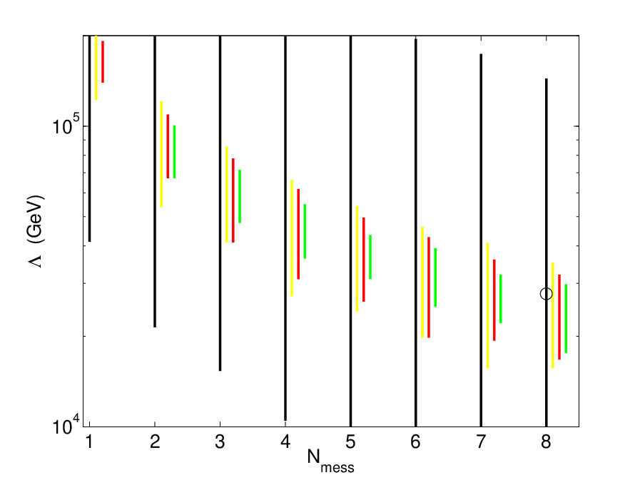
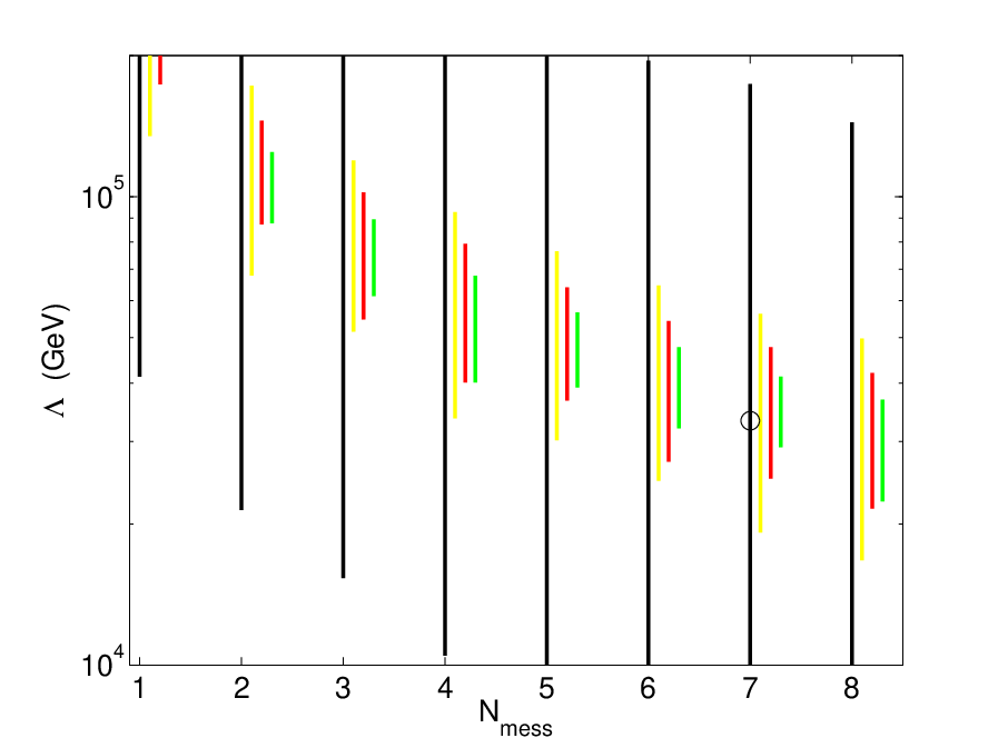
As for the CMSSM scenario also in mGMSB we have chosen a hypothetical future best-fit point with higher mass scales, defined by eq. (36). As for the CMSSM, we assume that the future experimental values agree exactly with the low-energy parameters corresponding to eq. (36). The reduction of the regions can be observed in Fig. 21. It is at the same level as for the current best-fit point in Fig. 20. These results are also shown in the – plane in Fig. 23, where the same sensitivity is found as for the current best-fit point displayed in Fig. 22.
5.1.3 mAMSB
In Fig. 24 we show the only high-energy parameter plane in the mAMSB, vs. , with the same color coding as in Fig. 7. Within this scenario the precision observables will allow an extremely precise determination of the high-energy parameters. For the case that the current best-fit point agrees exactly with the future measurements, at the level is determined to , i.e. to . The absolute precision for is , whereas the relative precision reaches only . (The and regions are very small and nearly invisible inside (by definition) the region.) This result is to a large extent due to the fact that the value for the current best-fit point is relatively low (see also the discussion of the hypothetical best-fit point below).
As for the other two scenarios, also in mAMSB we have chosen a hypothetical future best-fit point with higher mass scales, defined by eq. (37). It should be noted that for mAMSB the increase in from the current best-fit point to the hypothetical best-fit point is a bit smaller than in the other two scenarios, while the shift in is substantially larger. Again we assume that the future experimental values agree exactly with the low-energy parameters corresponding to eq. (37). We show the preferred parameter space for this hypothetical point in Fig. 25. The reduction in the size of the regions compared to the present situation is much weaker than for the current best-fit point in Fig. 24. At the level no limit on can be set. This shows that the very high precision obtainable with the current best-fit point is not generally valid in the mAMSB scenario.
5.2 Low-energy analysis
We now turn to the comparison of the three soft SUSY-breaking scenarios in terms of and , assuming the future experimental and theory precisions as discussed in Sect. 3. In Fig. 26 we show the – plane for the CMSSM (top), mGMSB (middle) and mAMSB (bottom) with the same color coding as in Fig. 7. In each scenario we assume that the future measurements will agree exactly with the current best-fit point.


A drastic improvement compared to the present situation can be observed in all three scenarios. However, also for the low-energy parameters the quality of the improvement going to the future sensitivities depends on the fact that currently relatively low mass scales are favored, see below. The results look quite different in mAMSB as compared to the CMSSM and mGMSB. Within the latter two the region is confined to with a width of for the CMSSM (mGMSB), whereas is only weakly restricted, . Within mAMSB, as for the high-energy parameters, a very precise indirect determination of and can be performed. At the level is confined to , i.e. to about 6%. is determined to , corresponding to a precision of . However, as discussed in Sect. 5.1.3, this is largely due to the relatively small value of within the mAMSB scenario at the current best-fit point.


We finally investigate the future sensitivity of the three soft SUSY-breaking scenarios for the hypothetical best-fit point. In Fig. 27 we show the results for the hypothetical best-fit points as defined in eqs. (35), (36), (37) for the CMSSM, mGMSB and mAMSB, respectively. By definition, see eq. (34), the hypothetical best-fit values for and are very similar in the three scenarios, and . These values are somewhat larger than the current best-fit values, see Tab. 1. In combination with such heavy MSSM Higgs bosons could not be detected at the LHC [145, 146, 147, 148, 149, 150, 152] or the ILC [125, 126, 127, 128]. Despite the fact that these values are already in the decoupling regime (i.e. where SUSY masses are large and loop effects are correspondingly small), the precision observables are still able to provide upper (and lower) limits on and with similar results in the three soft SUSY-breaking scenarios. The upper limit at the level on varies between in the CMSSM and in mGMSB. This means that the limits obtainable for and depend only to a small extent on the details of the underlying physics scenario and can thus be viewed as a more general result for scenarios resulting from a high-scale theory. In conclusion, the precision observables could allow one to set an indirect bound on (and mildly also on ) beyond the direct collider reach. This sensitivity would improve even more if the future collider data (SUSY masses etc.) would be included (see e.g. Ref. [155]). Such an analysis, however, would at the present state be highly speculative and is beyond the scope of our paper.
6 Conclusions
We investigated the constraints arising from electroweak precision observables (EWPO) and -physics observables (BPO) providing a comparison of the CMSSM, the mGMSB and the mAMSB. We performed a analysis based on the mass of the boson, , the effective weak leptonic mixing angle, , the anomalous magnetic moment of the muon , the mass of the lightest -even MSSM Higgs boson, , as well as on and . Our analysis should be viewed as an exploratory study for the comparison of the scenarios, providing a starting point for a more refined investigation using more precision data and an elaborate analysis [18].
Our results are analyzed separately in terms of the high-scale parameters of the respective model as well as in terms of low-energy parameters such as , and SUSY particle masses. Using todays measurements, uncertainties and exclusion bounds, we find that relatively low mass scales in all three scenarios are favored at the level of or 4. However, the current data of EWPO and BPO can hardly set any upper bound on the SUSY mass scales at the level of . The best fit-values for range from in the CMSSM up to in mAMSB, whereas the values are only weakly constrained. Remarkably the mAMSB scenario, despite having one free GUT scale parameter less than the other two scenarios, has a somewhat lower total minimum . This can be traced back to a better agreement with the combination of the and measurements (with some help from ) for a heavier scalar quark spectrum and a corresponding slightly larger value of .
We presented predictions for the lightest -even Higgs boson mass, based on the current data, but without imposing the current LEP bound from Higgs boson searches and its corresponding contribution. Best-fit values of are found for the CMSSM and mGMSB, and for mAMSB. In all three scenarios a relatively good compatibility with the direct bounds from the Higgs searches at LEP is found. Within mAMSB the region extends up to .
We also presented the predictions for the masses of various SUSY particles such as , , , , , , , , and in the three soft SUSY-breaking scenarios. As a general feature lowest masses are found in the mAMSB and heaviest in mGMSB. All three scenarios offer good prospects for the discovery of some color-neutral particles at the ILC (with a center-of-mass energy up to ) and for colored particles at the LHC. There are also good prospects for the discovery of uncolored particles such as charginos, neutralinos and light sleptons, especially if they are produced in cascade decays. Some part of the preferred parameter space in the three scenarios is currently probed at the Tevatron. Within the CMSSM qualitative agreement in the preferred mass ranges with previous analyses [11, 12, 13] has been found.
Finally, we explored the projection for the future sensitivities of the EWPO and BPO in the three soft SUSY-breaking scenarios. Here we also assumed a measurement of the lightest MSSM Higgs boson mass. In a first step we analyzed the future sensitivities assuming that the future measurements agree with the current best-fit results. We found a strong improvement with respect to the current sensitivity. Within the mAMSB scenario and can be determined indirectly with very high precision, largely due to the fact that the current best-fit point has a relatively low value. On the other hand, in the CMSSM and mGMSB the determination remains relatively weak, where the current best-fit points have very large values. In a second step we assumed that the future measurements will agree in each scenario with a certain hypothetical point. These three points were defined for each scenario such that they result in a similar Higgs and SUSY spectrum with and . In general the Higgs and SUSY mass scales are somewhat higher than for the current best-fit points, i.e. loop corrections are correspondingly somewhat smaller. These points would not permit a direct determination of the heavy Higgs-boson mass scale. We find that the EWPO and BPO exhibit a similar future sensitivity in the CMSSM, mGMSB and mAMSB giving rise to an upper limit on the high-scale parameters at the level. The future EWPO and BPO sensitivities depend only mildly on the underlying physics scenario. The precision observables could allow one to constrain the Higgs sector parameters even beyond the direct reach of the LHC or the ILC.
Once LHC (and ILC) data on SUSY masses will be available, the assumption about the underlying scenario itself will be investigated. While information from the direct production of SUSY particles will obviously be crucial for disentangling the underlying scenario of SUSY-breaking, also the EWPO and BPO will certainly play an important role in this context.
Acknowledgements
We thank B. Allanach for help with in the use of SoftSUSY. We thank A. Dedes and C.E.M. Wagner for helpful discussions. The work of S.H. was partially supported by CICYT (grant FPA 2007–66387). X.M. and S.S. are supported under U.S. Department of Energy contract # DE-FG02-04ER-41298. Work supported in part by the European Community’s Marie-Curie Research Training Network under contract MRTN-CT-2006-035505 ‘Tools and Precision Calculations for Physics Discoveries at Colliders’.
References
- [1] H. Nilles, Phys. Rept. 110 (1984) 1.
- [2]
H. Haber and G. Kane,
Phys. Rept. 117 (1985) 75;
R. Barbieri, Riv. Nuovo Cim. 11 (1988) 1. - [3] Heavy Flavor Analysis group, see: www.slac.stanford.edu/xorg/hfag/ .
- [4]
J. Ellis, S. Kelley and D. Nanopoulos,
Phys. Lett. B 260 (1991) 131;
U. Amaldi, W. de Boer and H. Furstenau, Phys. Lett. B 260 (1991) 447;
C. Giunti, C. Kim and U. Lee, Mod. Phys. Lett. A 6 (1991) 1745. - [5]
M. Dine, W. Fischler and M. Srednicki,
Nucl. Phys. B 189 (1981) 575;
S. Dimopoulos and S. Raby, Nucl. Phys. B 192 (1981) 353;
M. Dine and W. Fischler, Phys. Lett. B 110 (1982) 227;
M. Dine and M. Srednicki, Nucl. Phys. B 202 (1982) 238;
M. Dine and W. Fischler, Nucl. Phys. B 204 (1982) 346;
L. Alvarez-Gaumé, M. Claudson and M. Wise, Nucl. Phys. B 207 (1982) 96;
C. Nappi and B. Ovrut, Phys. Lett. B 113 (1982) 175;
S. Dimopoulos and S. Raby, Nucl. Phys. B 219 (1983) 479. - [6]
M. Dine and A. Nelson,
Phys. Rev. D 48 (1993) 1277
[arXiv:hep-ph/9303230];
M. Dine, A. Nelson and Y. Shirman, Phys. Rev. D 51 (1995) 1362 [arXiv:hep-ph/9408384];
M. Dine, A. Nelson, Y. Nir and Y. Shirman, Phys. Rev. D 53 (1996) 2658 [arXiv:hep-ph/9507378]. - [7] For a review, see: G. Giudice and R. Rattazzi, Phys. Rept. 322 (1999) 419 [arXiv:hep-ph/9801271].
- [8] L. Randall and R. Sundrum, Nucl. Phys. B 557 (1999) 79 [arXiv:hep-th/9810155].
- [9] G. Giudice, M. Luty, H. Murayama and R. Rattazzi, JHEP 9812 (1998) 027 [arXiv:hep-ph/9810442].
- [10] T. Gherghetta, G. Giudice and J. Wells, Nucl. Phys. B 559 (1999) 27 [arXiv:hep-ph/9904378].
- [11] J. Ellis, S. Heinemeyer, K. Olive and G. Weiglein, JHEP 0502 (2005) 013 [arXiv:hep-ph/0411216].
- [12] J. Ellis, S. Heinemeyer, K. Olive and G. Weiglein, JHEP 0605 (2006) 005 [arXiv:hep-ph/0602220].
- [13] J. Ellis, S. Heinemeyer, K. Olive, A.M. Weber and G. Weiglein, JHEP 0708 (2007) 083 [arXiv:0706.0652 [hep-ph]].
- [14] J. Ellis, T. Hahn, S. Heinemeyer, K. Olive and G. Weiglein, JHEP 0710 (2007) 092 [arXiv:0709.0098 [hep-ph]].
- [15] J. Ellis, S. Heinemeyer, K. Olive and G. Weiglein, Phys. Lett. B 653 (2007) 292 [arXiv:0706.0977 [hep-ph]].
- [16]
J. Ellis, K. Olive, Y. Santoso and V. Spanos,
Phys. Rev. D 69 (2004) 095004
[arXiv:hep-ph/0310356];
B. Allanach and C. Lester, Phys. Rev. D 73 (2006) 015013 [arXiv:hep-ph/0507283];
B. Allanach, Phys. Lett. B 635 (2006) 123 [arXiv:hep-ph/0601089];
R. de Austri, R. Trotta and L. Roszkowski, JHEP 0605 (2006) 002 [arXiv:hep-ph/0602028]; JHEP 0704 (2007) 084 [arXiv:hep-ph/0611173]; JHEP 0707 (2007) 075 [arXiv:0705.2012 [hep-ph]];
B. Allanach, C. Lester and A. M. Weber, JHEP 0612 (2006) 065 [arXiv:hep-ph/0609295]; JHEP 0708 (2007) 023 [arXiv:0705.0487 [hep-ph]];
S. Heinemeyer, arXiv:hep-ph/0611372. - [17]
G. Isidori, F. Mescia, P. Paradisi and D. Temes,
Phys. Rev. D 75 (2007) 115019
[arXiv:hep-ph/0703035];
M. Carena, A. Menon and C. Wagner, Phys. Rev. D 76 (2007) 035004 [arXiv:0704.1143 [hep-ph]]. - [18] O. Buchmueller et al., Phys. Lett. B 657 (2007) 87 [arXiv:0707.3447 [hep-ph]].
- [19]
S. Heinemeyer, M. Mondragón and G. Zoupanos,
arXiv:0712.3630 [hep-ph];
A. Djouadi, S. Heinemeyer, M. Mondragón and G. Zoupanos, Springer Proc. Phys. 98 (2005) 273 [arXiv:hep-ph/0404208]. - [20] F. Mahmoudi, JHEP 0712 (2007) 026 [arXiv:0710.3791 [hep-ph]].
- [21] F. Domingo and U. Ellwanger, JHEP 0712 (2007) 090 [arXiv:0710.3714 [hep-ph]].
- [22] J. Kasahara, K. Freese and P. Gondolo, arXiv:0805.0999 [hep-ph].
- [23]
C. Bennett et al.,
Astrophys. J. Suppl. 148 (2003) 1
[arXiv:astro-ph/0302207];
D. Spergel et al. [WMAP Collaboration], Astrophys. J. Suppl. 148 (2003) 175 [arXiv:astro-ph/0302209];
D. Spergel et al. [WMAP Collaboration], Astrophys. J. Suppl. 170 (2007) 377 [arXiv:astro-ph/0603449]. - [24] A. Arbey and F. Mahmoudi, arXiv:0803.0741 [hep-ph].
- [25]
H. Dreiner,
arXiv:hep-ph/9707435;
G. Bhattacharyya, arXiv:hep-ph/9709395;
B. Allanach, A. Dedes and H. Dreiner, Phys. Rev. D 60 (1999) 075014 [arXiv:hep-ph/9906209]. - [26] D. Lyth and E. Stewart, Phys. Rev. D 53 (1996) 1784 [arXiv:hep-ph/9510204].
- [27] G. Gelmini and P. Gondolo, Phys. Rev. D 74 (2006) 023510 [arXiv:hep-ph/0602230].
- [28]
G. Degrassi, P. Gambino and P. Slavich,
Phys. Lett. B 635 (2006) 335
[arXiv:hep-ph/0601135];
E. Lunghi, W. Porod and O. Vives, Phys. Rev. D 74 (2006) 075003 [arXiv:hep-ph/0605177]. - [29]
H. Nilles,
Phys. Lett. B 115 (1982) 193;
Nucl. Phys. B 217 (1983) 366;
A. Chamseddine, R. Arnowitt and P. Nath, Phys. Rev. Lett. 49 (1982) 970;
R. Barbieri, S. Ferrara and C. Savoy, Phys. Lett. B 119 (1982) 343;
H. Nilles, M. Srednicki and D. Wyler, Phys. Lett. B 120 (1983) 346;
E. Cremmer, P. Fayet and L. Girardello, Phys. Lett. B 122 (1983) 41;
S. Ferrara, L. Girardello and H. Nilles, Phys. Lett. B 125 (1983) 457;
L. Hall, J. Lykken and S. Weinberg, Phys. Rev. D 27 (1983) 2359;
S. Soni and H. Weldon, Phys. Lett. B 126 (1983) 215;
R. Arnowitt, A. Chamseddine and P. Nath, Nucl. Phys. B 227 (1983) 121.
For more details see, S. Weinberg, “The quantum theory of fields. Vol. 3: Supersymmetry,” Cambridge University Press (2000). - [30]
For reviews see also:
Ref. [1] and the first article in Ref. [2];
A. Lahanas and D. Nanopoulos, Phys. Rept. 145 (1987) 1;
S. Martin, in “Perspectives on supersymmetry”, ed. G. Kane, arXiv:hep-ph/9709356, see: zippy.physics.niu.edu/primer.shtml. - [31] H. Murayama and Y. Nomura, Phys. Rev. Lett. 98 (2007) 151803 [arXiv:hep-ph/0612186]; Phys. Rev. D 75 (2007) 095011 [arXiv:hep-ph/0701231].
- [32] S. Abel, C. Durnford, J. Jaeckel and V. V. Khoze, JHEP 0802 (2008) 074 [arXiv:0712.1812 [hep-ph]].
- [33] W. Yao et al. [Particle Data Group Collaboration], J. Phys. G 33 (2006) 1.
- [34] P. Fayet, Phys. Lett. B 70 (1977) 461; Phys. Lett. B 86 (1979) 272; Phys. Lett. B 175 (1986) 471; and in “Unification of the fundamental particle interactions”, eds. S. Ferrara, J. Ellis, P. van Nieuwenhuizen (Plenum, New York, 1980) p. 587.
- [35] A. Pomarol and R. Rattazzi, JHEP 9905 (1999) 013 [arXiv:hep-ph/9903448].
- [36] Z. Chacko, M. Luty and E. Ponton, JHEP 0004 (2000) 001 [arXiv:hep-ph/9905390].
- [37] E. Katz, Y. Shadmi and Y. Shirman, JHEP 9908 (1999) 015 [arXiv:hep-ph/9906296].
- [38] I. Jack, D. Jones and R. Wild, Phys. Lett. B 535, 193 (2002) [arXiv:hep-ph/0202101].
- [39] B. Allanach, Comput. Phys. Commun. 143 (2002) 305 [arXiv:hep-ph/0104145].
- [40] S. Heinemeyer, W. Hollik and G. Weiglein, Phys. Rept. 425 (2006) 265 [arXiv:hep-ph/0412214].
- [41] S. Heinemeyer, W. Hollik, A.M. Weber and G. Weiglein, JHEP 0804 (2008) 039 [arXiv:0710.2972 [hep-ph]].
- [42]
E. Brubaker et al. [Tevatron Electroweak Working Group],
arXiv:hep-ex/0608032,
see: tevewwg.fnal.gov/top/ . - [43]
Tevatron Electroweak Working Group,
axXiv:0803.1683 [hep-ex];
see: tevewwg.fnal.gov/top/ . - [44]
A. Sirlin,
Phys. Rev. D 22 (1980) 971;
W. Marciano and A. Sirlin, Phys. Rev. D 22 (1980) 2695. - [45] P. Chankowski, A. Dabelstein, W. Hollik, W. Mösle, S. Pokorski and J. Rosiek, Nucl. Phys. B 417 (1994) 101.
- [46] D. Garcia and J. Solà, Mod. Phys. Lett. A 9 (1994) 211.
- [47]
A. Djouadi and C. Verzegnassi,
Phys. Lett. B 195 (1987) 265;
A. Djouadi, Nuovo Cim. A 100 (1988) 357. - [48]
B. Kniehl,
Nucl. Phys. B 347 (1990) 89;
F. Halzen and B. Kniehl, Nucl. Phys. B 353 (1991) 567;
B. Kniehl and A. Sirlin, Nucl. Phys. B 371 (1992) 141; Phys. Rev. D 47 (1993) 883. - [49]
K. Chetyrkin, J. Kühn and M. Steinhauser,
Phys. Rev. Lett. 75 (1995) 3394
[arXiv:hep-ph/9504413];
L. Avdeev et al., Phys. Lett. B 336 (1994) 560, [Erratum-ibid. B 349 (1995) 597] [arXiv:hep-ph/9406363]. - [50] K. Chetyrkin, J. Kühn and M. Steinhauser, Nucl. Phys. B 482 (1996) 213 [arXiv:hep-ph/9606230].
- [51] A. Djouadi, P. Gambino, S. Heinemeyer, W. Hollik, C. Jünger and G. Weiglein, Phys. Rev. Lett. 78 (1997) 3626 [arXiv:hep-ph/9612363]; Phys. Rev. D 57 (1998) 4179 [arXiv:hep-ph/9710438].
- [52] S. Heinemeyer and G. Weiglein, JHEP 0210 (2002) 072 [arXiv:hep-ph/0209305]; arXiv:hep-ph/0301062.
- [53] J. Haestier, S. Heinemeyer, D. Stöckinger and G. Weiglein, JHEP 0512 (2005) 027 [arXiv:hep-ph/0508139]; arXiv:hep-ph/0506259.
- [54] M. Veltman, Nucl. Phys. B 123 (1977) 89.
- [55] S. Heinemeyer, W. Hollik, D. Stöckinger, A.M. Weber and G. Weiglein, JHEP 0608 (2006) 052 [arXiv:hep-ph/0604147]; arXiv:hep-ph/0611371.
- [56] A. Hoang et al., Eur. Phys. J. direct C 2 (2000) 1 [arXiv:hep-ph/0001286].
- [57] M. Martinez and R. Miquel, Eur. Phys. J. C 27 (2003) 49 [arXiv:hep-ph/0207315].
- [58]
F. Jegerlehner,
Talk presented at the LNF Spring School,
Frascati, Italy, 1999,
see: www-com.physik.hu-berlin.de/fjeger/Frascati99.ps.gz ;
arXiv:hep-ph/0105283. - [59] S. Heinemeyer, S. Kraml, W. Porod and G. Weiglein, JHEP 0309 (2003) 075 [arXiv:hep-ph/0306181].
- [60]
The ALEPH, DELPHI, L3, OPAL, SLD Collaborations,
the LEP Electroweak Working Group,
the SLD Electroweak and Heavy Flavour Groups,
arXiv:hep-ex/0509008;
[The ALEPH, DELPHI, L3 and OPAL Collaborations, the LEP Electroweak Working Group], arXiv:hep-ex/0612034. - [61]
LEP Electroweak Working Group,
see: lepewwg.web.cern.ch/LEPEWWG/Welcome.html. - [62] Tevatron Electroweak Working Group, see: tevewwg.fnal.gov .
- [63]
CDF collaboration,
arXiv:0707.0085 [hep-ex];
see: www-cdf.fnal.gov/physics/ewk/ . - [64] M. Grünewald, private communication.
- [65] S. Brensing, S. Dittmaier, M. Krämer and A. Mück, Phys. Rev. D 77 (2008) 073006 [arXiv:0710.3309 [hep-ph]].
- [66] G. Wilson, LC-PHSM-2001-009, see: www.desy.de/lcnotes/notes.html .
- [67] U. Baur, R. Clare, J. Erler, S. Heinemeyer, D. Wackeroth, G. Weiglein and D. Wood, arXiv:hep-ph/0111314.
- [68] M. Awramik, M. Czakon, A. Freitas and G. Weiglein, Phys. Rev. Lett. 93 (2004) 201805 [arXiv:hep-ph/0407317].
- [69] R. Hawkings and K. Mönig, Eur. Phys. J. direct C 8 (1999) 1 [arXiv:hep-ex/9910022].
- [70] J. Erler, S. Heinemeyer, W. Hollik, G. Weiglein and P. Zerwas, Phys. Lett. B 486 (2000) 125 [arXiv:hep-ph/0005024].
- [71] A. Czarnecki and W. Marciano, Phys. Rev. D 64 (2001) 013014 [arXiv:hep-ph/0102122].
- [72]
M. Knecht,
Lect. Notes Phys. 629 (2004) 37
[arXiv:hep-ph/0307239];
M. Passera, Nucl. Phys. Proc. Suppl. 155 (2006) 365 [arXiv:hep-ph/0509372]. - [73] D. Stöckinger, J. Phys. G 34 (2007) R45 [arXiv:hep-ph/0609168].
- [74] J. Miller, E. de Rafael and B. Roberts, Rept. Prog. Phys. 70 (2007) 795 [arXiv:hep-ph/0703049].
- [75] F. Jegerlehner, Acta Phys. Polon. B 38 (2007) 3021 [arXiv:hep-ph/0703125].
- [76] M. Passera, W. Marciano and A. Sirlin, arXiv:0804.1142 [hep-ph].
- [77] T. Kinoshita and M. Nio, Phys. Rev. D 70 (2004) 113001 [arXiv:hep-ph/0402206]; Phys. Rev. 73 (2006) 053007 [arXiv:hep-ph/0512330].
- [78] M. Passera, Phys. Rev. D 75 (2007) 013002 [arXiv:hep-ph/0606174].
- [79] T. Aoyama, M. Hayakawa, T. Kinoshita and M. Nio, Phys. Rev. Lett. 99 (2007) 110406 [arXiv:0706.3496 [hep-ph]]; Nucl. Phys. B 796 (2008) 184 [arXiv:0709.1568 [hep-ph]]; arXiv:0712.2607 [hep-ph].
- [80] M. Davier, S. Eidelman, A. Höcker and Z. Zhang, Eur. Phys. J. C 31 (2003) 503 [arXiv:hep-ph/0308213].
- [81] K. Hagiwara, A. Martin, D. Nomura and T. Teubner, Phys. Rev. D 69 (2004) 093003 [arXiv:hep-ph/0312250].
- [82] K. Hagiwara, A. Martin, D. Nomura and T. Teubner, Phys. Lett. B 649 (2007) 173 [arXiv:hep-ph/0611102].
- [83] S. Ghozzi and F. Jegerlehner, Phys. Lett. B 583 (2004) 222 [arXiv:hep-ph/0310181].
- [84] J. de Troconiz and F. Yndurain, Phys. Rev. D 71 (2005) 073008 [arXiv:hep-ph/0402285].
- [85] M. Davier, Nucl. Phys. Proc. Suppl. 169 (2007) 288 [arXiv:hep-ph/0701163].
- [86] J. Bijnens and J. Prades, Mod. Phys. Lett. A 22 (2007) 767 [arXiv:hep-ph/0702170].
- [87]
M. Knecht and A. Nyffeler,
Phys. Rev. D 65 (2002) 073034
[arXiv:hep-ph/0111058];
M. Knecht, A. Nyffeler, M. Perrottet and E. De Rafael, Phys. Rev. Lett. 88 (2002) 071802 [arXiv:hep-ph/0111059];
I. Blokland, A. Czarnecki and K. Melnikov, Phys. Rev. Lett. 88 (2002) 071803 [arXiv:hep-ph/0112117];
M. Ramsey-Musolf and M. Wise, Phys. Rev. Lett. 89 (2002) 041601 [arXiv:hep-ph/0201297];
J. Kühn, A. Onishchenko, A. Pivovarov and O. Veretin, Phys. Rev. D 68 (2003) 033018 [arXiv:hep-ph/0301151]. - [88] K. Melnikov and A. Vainshtein, Phys. Rev. D 70 (2004) 113006 [arXiv:hep-ph/0312226].
- [89] M. Davier and W. Marciano, Ann. Rev. Nucl. Part. Sci. 54 (2004) 115.
- [90] H. Hayashii [Belle Collaboration], PoS HEP2005 (2006) 291.
- [91] M. Benayoun, P. David, L. DelBuono, O. Leitner and H. O’Connell, arXiv:0711.4482 [hep-ph].
- [92]
A. Aloisio et al. [KLOE Collaboration],
Phys. Lett. 606 (2005) 12
[arXiv:hep-ex/0407048];
D. Leone [KLOE Collaboration], Nucl. Phys. Proc. Suppl. 162 (2006) 95. - [93] R. Akhmetshin et al. [CMD-2 Collaboration], Phys. Lett. B 578 (2004) 285 [arXiv:hep-ex/0308008]; Phys. Lett. B 648 (2007) 28 [arXiv:hep-ex/0610021].
- [94] M. Achasov et al. [SND Collaboration], J. Exp. Theor. Phys. 101 (2005) 1053 [arXiv:hep-ex/0506076].
- [95]
S. Müller,
talk given at the EPS07, Manchester, July 2007, see:
agenda.hep.man.ac.uk/contribution
Display.py?contribId=36&sessionId=26&confId=70 . - [96] G. Bennett et al. [The Muon g-2 Collaboration], Phys. Rev. Lett. 92 (2004) 161802 [arXiv:hep-ex/0401008].
- [97] G. Bennett et al. [The Muon g-2 Collaboration], Phys. Rev. D 73 (2006) 072003 [arXiv:hep-ex/0602035].
- [98]
S. Eidelman,
talk given at the ICHEP06, Moscow, July 2006,
see: ichep06.jinr.ru/reports/333_6s1_9p30_Eidelman.pdf ;
V. Druzhinin, talk given at Lepton Photon 07, August 2007, Daegu, Korea,
see: chep.knu.ac.kr/lp07/htm/S5/S05-15.pdf . - [99] T. Moroi, Phys. Rev. D 53 (1996) 6565 [Erratum-ibid. D 56 (1997) 4424] [arXiv:hep-ph/9512396].
- [100]
J. Lopez, D. Nanopoulos and X. Wang,
Phys. Rev. D 49 (1994) 366
[arXiv:hep-ph/9308336];
U. Chattopadhyay and P. Nath, Phys. Rev. D 53 (1996) 1648 [arXiv:hep-ph/9507386]. - [101] G. Degrassi and G. Giudice, Phys. Rev. D 58 (1998) 053007 [arXiv:hep-ph/9803384].
- [102] S. Heinemeyer, D. Stöckinger and G. Weiglein, Nucl. Phys. B 690 (2004) 62 [arXiv:hep-ph/0312264].
- [103] S. Heinemeyer, D. Stöckinger and G. Weiglein, Nucl. Phys. B 699 (2004) 103 [arXiv:hep-ph/0405255].
- [104] A. Dabelstein, Nucl. Phys. B 456 (1995) 25 [arXiv:hep-ph/9503443]; Z. Phys. C 67 (1995) 495 [arXiv:hep-ph/9409375].
- [105] S. Heinemeyer, W. Hollik and G. Weiglein, Phys. Rev. D 58 (1998) 091701 [arXiv:hep-ph/9803277]; Phys. Lett. B 440 (1998) 296 [arXiv:hep-ph/9807423].
- [106] S. Heinemeyer, W. Hollik and G. Weiglein, Comput. Phys. Commun. 124 2000 76 [arXiv:hep-ph/9812320]. The code is accessible via www.feynhiggs.de .
- [107] S. Heinemeyer, W. Hollik and G. Weiglein, Eur. Phys. J. C 9 (1999) 343 [arXiv:hep-ph/9812472].
- [108] G. Degrassi, S. Heinemeyer, W. Hollik, P. Slavich, G. Weiglein, Eur. Phys. J. C 28 (2003) 133 [arXiv:hep-ph/0212020].
- [109] M. Frank, T. Hahn, S. Heinemeyer, W. Hollik, H. Rzehak and G. Weiglein, JHEP 0702 (2007) 047 [arXiv:hep-ph/0611326].
- [110]
Y. Okada, M. Yamaguchi, T. Yanagida,
Prog. Theor. Phys. 85 (1991) 1;
J. Ellis, G. Ridolfi, F. Zwirner, Phys. Lett. B 257 (1991) 83;
H. Haber, R. Hempfling, Phys. Rev. Lett. 66 (1991) 1815. - [111] P. Chankowski, S. Pokorski, J. Rosiek, Phys. Lett. B 286 (1992) 307; Nucl. Phys. B 423 (1994) 437 [arXiv:hep-ph/9303309].
- [112]
M. Carena, D. Garcia, U. Nierste and C. Wagner,
Nucl. Phys. B 577 (2000) 577
[arXiv:hep-ph/9912516];
H. Eberl, K. Hidaka, S. Kraml, W. Majerotto and Y. Yamada, Phys. Rev. D 62 (2000) 055006 [arXiv:hep-ph/9912463]. - [113]
T. Banks,
Nucl. Phys. B 303 (1988) 172;
L. Hall, R. Rattazzi and U. Sarid, Phys. Rev. D 50 (1994) 7048 [arXiv:hep-ph/9306309];
R. Hempfling, Phys. Rev. D 49 (1994) 6168;
M. Carena, M. Olechowski, S. Pokorski and C. Wagner, Nucl. Phys. B 426 (1994) 269 [arXiv:hep-ph/9402253]. - [114] G. Degrassi, A. Dedes and P. Slavich, Nucl. Phys. B 672 (2003) 144 [arXiv:hep-ph/0305127].
- [115]
S. Martin,
Phys. Rev. D 65 (2002) 116003
[arXiv:hep-ph/0111209];
Phys. Rev. D 66 (2002) 096001
[arXiv:hep-ph/0206136];
Phys. Rev. D 67 (2003) 095012
[arXiv:hep-ph/0211366];
Phys. Rev. D 68 075002 (2003)
[arXiv:hep-ph/0307101];
Phys. Rev. D 70 (2004) 016005
[arXiv:hep-ph/0312092];
Phys. Rev. D 71 (2005) 016012
[arXiv:hep-ph/0405022];
Phys. Rev. D 71 (2005) 116004
[arXiv:hep-ph/0502168];
S. Martin and D. Robertson, Comput. Phys. Commun. 174 (2006) 133 [arXiv:hep-ph/0501132]. - [116] S. Martin, Phys. Rev. D 75 (2007) 055005 [arXiv:hep-ph/0701051].
- [117] R. Harlander, P. Kant, L. Mihaila and M. Steinhauser, arXiv:0803.0672 [hep-ph].
- [118] S. Heinemeyer, W. Hollik, H. Rzehak and G. Weiglein, Eur. Phys. J. C 39 (2005) 465 [arXiv:hep-ph/0411114]; arXiv:hep-ph/0506254.
- [119] B. Allanach, A. Djouadi, J. Kneur, W. Porod and P. Slavich, JHEP 0409 (2004) 044 [arXiv:hep-ph/0406166].
- [120] S. Heinemeyer, W. Hollik and G. Weiglein, JHEP 0006 (2000) 009 [arXiv:hep-ph/9909540].
- [121] LEP Higgs working group, Eur. Phys. J. C 47 (2006) 547 [arXiv:hep-ex/0602042].
- [122] LEP Higgs working group, Phys. Lett. B 565 (2003) 61 [arXiv:hep-ex/0306033].
- [123] S. Ambrosanio, A. Dedes, S. Heinemeyer, S. Su and G. Weiglein, Nucl. Phys. B 624 (2001) 3 [arXiv:hep-ph/0106255].
- [124] J. Ellis, S. Heinemeyer, K. Olive and G. Weiglein, Phys. Lett. B 515 (2001) 348 [arXiv:hep-ph/0105061].
- [125] J. Aguilar-Saavedra et al., TESLA TDR Part 3: “Physics at an Linear Collider”, arXiv:hep-ph/0106315, see: tesla.desy.de/tdr/ .
- [126] T. Abe et al. [American Linear Collider Working Group Collaboration], Resource book for Snowmass 2001, arXiv:hep-ex/0106055.
- [127] K. Abe et al. [ACFA Linear Collider Working Group Collaboration], arXiv:hep-ph/0109166.
- [128] S. Heinemeyer et al., arXiv:hep-ph/0511332.
- [129] M. Misiak et al., Phys. Rev. Lett. 98 (2007) 022002 [arXiv:hep-ph/0609232].
- [130] T. Hurth, E. Lunghi and W. Porod, Nucl. Phys. B 704 (2005) 56 [arXiv:hep-ph/0312260].
- [131] M. Neubert, Eur. Phys. J. C 40 (2005) 165 [arXiv:hep-ph/0408179].
- [132]
R. Barate et al. [ALEPH Collaboration],
Phys. Lett. B 429 (1998) 169;
S. Chen et al. [CLEO Collaboration], Phys. Rev. Lett. 87 (2001) 251807 [arXiv:hep-ex/0108032];
P. Koppenburg et al. [Belle Collaboration], Phys. Rev. Lett. 93 (2004) 061803 [arXiv:hep-ex/0403004];
K. Abe et al. [Belle Collaboration], Phys. Lett. B 511 (2001) 151 [arXiv:hep-ex/0103042];
B. Aubert et al. [BABAR Collaboration], arXiv:hep-ex/0207074; arXiv:hep-ex/0207076. - [133]
P. Cho, M. Misiak and D. Wyler,
Phys. Rev. D 54, 3329 (1996)
[arXiv:hep-ph/9601360];
A. Kagan and M. Neubert, Eur. Phys. J. C 7 (1999) 5 [arXiv:hep-ph/9805303];
A. Ali, E. Lunghi, C. Greub and G. Hiller, Phys. Rev. D 66 (2002) 034002 [arXiv:hep-ph/0112300];
G. Hiller and F. Krüger, Phys. Rev. D 69 (2004) 074020 [arXiv:hep-ph/0310219];
M. Carena, D. Garcia, U. Nierste and C. Wagner, Phys. Lett. B 499 (2001) 141 [arXiv:hep-ph/0010003];
D. Demir and K. Olive, Phys. Rev. D 65 (2002) 034007 [arXiv:hep-ph/0107329];
T. Hurth, arXiv:hep-ph/0212304. - [134]
K. Adel and Y. Yao,
Phys. Rev. D 49 (1994) 4945
[arXiv:hep-ph/9308349];
C. Greub, T. Hurth and D. Wyler, Phys. Lett. B 380 (1996) 385 [arXiv:hep-ph/9602281]; Phys. Rev. D 54 (1996) 3350 [arXiv:hep-ph/9603404];
A. Ali, talk given at ICHEP04, Beijing, August 2004, appeared in the proceedings, see: ichep04.ihep.ac.cn/db/paper.php . - [135] K. Chetyrkin, M. Misiak and M. Münz, Phys. Lett. B 400, (1997) 206 [Erratum-ibid. B 425 (1998) 414] [arXiv:hep-ph/9612313].
- [136] G. Belanger, F. Boudjema, A. Pukhov and A. Semenov, Comput. Phys. Commun. 149 (2002) 103 [arXiv:hep-ph/0112278]; arXiv:hep-ph/0405253.
- [137] C. Degrassi, P. Gambino and G. Giudice, JHEP 0012 (2000) 009 [arXiv:hep-ph/0009337].
- [138] P. Gambino and M. Misiak, Nucl. Phys. B 611 (2001) 338 [arXiv:hep-ph/0104034].
- [139]
G. Buchalla and A. Buras,
Nucl. Phys. B 400 (1993) 225;
M. Misiak and J. Urban, Phys. Lett. B 451 (1999) 161 [arXiv:hep-ph/9901278];
G. Buchalla and A. Buras, Nucl. Phys. B 548 (1999) 309 [arXiv:hep-ph/9901288];
A. Buras, Phys. Lett. B 566 (2003) 115 [arXiv:hep-ph/0303060]. - [140]
[CDF Collaboration],
arXiv:0712.1708 [hep-ex];
K. Tollefson talk given at Lepton Photon 07, August 2007, Daegu, Korea, see:
chep.knu.ac.kr/lp07/htm/S4/S04_14.pdf . - [141] CDF Collaboration, see: www-cdf.fnal.gov/physics/projections/ .
- [142] P. Ball et al., arXiv:hep-ph/0003238.
- [143]
K. Babu and C. Kolda,
Phys. Rev. Lett. 84 (2000) 228
[arXiv:hep-ph/9909476];
S. Choudhury and N. Gaur, Phys. Lett. B 451 (1999) 86 [arXiv:hep-ph/9810307];
C. Bobeth, T. Ewerth, F. Krüger and J. Urban, Phys. Rev. D 64 (2001) 074014 [arXiv:hep-ph/0104284];
A. Dedes, H. Dreiner and U. Nierste, Phys. Rev. Lett. 87 (2001) 251804 [arXiv:hep-ph/0108037];
G. Isidori and A. Retico, JHEP 0111 (2001) 001 [arXiv:hep-ph/0110121];
A. Dedes and A. Pilaftsis, Phys. Rev. D 67 (2003) 015012 [arXiv:hep-ph/0209306];
A. Buras, P. Chankowski, J. Rosiek and L. Slawianowska, Nucl. Phys. B 659 (2003) 3 [arXiv:hep-ph/0210145];
A. Dedes, Mod. Phys. Lett. A 18 (2003) 2627 [arXiv:hep-ph/0309233]. - [144] J. Ellis, K. Olive and V. Spanos, Phys. Lett. B 624 (2005) 47 [arXiv:hep-ph/0504196].
- [145]
ATLAS Collaboration,
Detector and Physics Performance Technical Design Report,
CERN/LHCC/99-15 (1999),
see: atlasinfo.cern.ch/Atlas/GROUPS/PHYSICS/TDR/access.html . - [146] CMS Collaboration, Physics Technical Design Report, Volume 2. CERN/LHCC 2006-021, see: cmsdoc.cern.ch/cms/cpt/tdr/ .
- [147] V. Büscher and K. Jakobs, Int. J. Mod. Phys. A 20 (2005) 2523 [arXiv:hep-ph/0504099].
- [148] M. Schumacher, Czech. J. Phys. 54 (2004) A103; arXiv:hep-ph/0410112.
- [149] S. Abdullin et al., Eur. Phys. J. C 39S2 (2005) 41.
- [150]
S. Gennai, S. Heinemeyer, A. Kalinowski, R. Kinnunen,
S. Lehti, A. Nikitenko and G. Weiglein,
Eur. Phys. J. C 52 (2007) 383
[arXiv:0704.0619 [hep-ph]];
M. Hashemi, S. Heinemeyer, R. Kinnunen, A. Nikitenko and G. Weiglein, arXiv:0804.1228 [hep-ph]. - [151]
J. Feng, T. Moroi, L. Randall, M. Strassler and S. Su,
Phys. Rev. Lett. 83 (1999) 1731
[arXiv:hep-ph/9904250];
S. Asai, T. Moroi and T. Yanagida, arXiv:0802.3725 [hep-ph]. - [152] F. Gianotti et al., Eur. Phys. J. C 39 (2005) 293 [arXiv:hep-ph/0204087].
- [153] J. Ellis, K. Olive, Y. Santoso and V. Spanos, Phys. Lett. B 565 (2003) 176 [arXiv:hep-ph/0303043].
- [154]
U. Chattopadhyay, A. Corsetti and P. Nath,
Phys. Rev. D 68 (2003) 035005
[arXiv:hep-ph/0303201];
H. Baer and C. Balazs, JCAP 0305 (2003) 006 [arXiv:hep-ph/0303114];
A. Lahanas and D. Nanopoulos, Phys. Lett. B 568 (2003) 55 [arXiv:hep-ph/0303130];
R. Arnowitt, B. Dutta and B. Hu arXiv:hep-ph/0310103. - [155] K. Desch, E. Gross, S. Heinemeyer, G. Weiglein and L. Zivkovic, JHEP 0409 (2004) 062 [arXiv:hep-ph/0406322].