Stochastic expansions and Hopf algebras

Simon J.A. Malham and Anke Wiese Affiliation: Maxwell Institute for Mathematical Sciences and School of Mathematical and Computer Sciences, Heriot-Watt University, Edinburgh EH14 4AS, UK
Dedicated to Mrs Jeanne Anne Malham
(17th April 2009)

Abstract

Stochastic expansions, Hopf algebras, numerical approximation We study solutions to nonlinear stochastic differential systems driven by a multi-dimensional Wiener process. A useful algorithm for strongly simulating such stochastic systems is the Castell–Gaines method, which is based on the exponential Lie series. When the diffusion vector fields commute, it has been proved that at low orders this method is more accurate in the mean-square error than corresponding stochastic Taylor methods. However it has also been shown that when the diffusion vector fields do not commute, this is not true for strong order one methods. Here we prove that when there is no drift, and the diffusion vector fields do not commute, the exponential Lie series is usurped by the sinh-log series. In other words, the mean-square error associated with a numerical method based on the sinh-log series, is always smaller than the corresponding stochastic Taylor error, in fact to all orders. Our proof utilizes the underlying Hopf algebra structure of these series, and a two-alphabet associative algebra of shuffle and concatenation operations. We illustrate the benefits of the proposed series in numerical studies.

1 Introduction

We are interested in designing strong series solutions of nonlinear Stratonovich stochastic differential systems of the form

y_{t}=y_{0}+\sum_{i=1}^{d}\int_{0}^{t}V_{i}(y_{\tau})\,\mathrm{d}W_{\tau}^{i}.

Here $(W^{1},\ldots,W^{d})$ is a $d$ -dimensional Wiener process and $y_{t}\in\mathbb{R}^{N}$ for some $N\in\mathbb{N}$ and all $t\in\mathbb{R}_{+}$ . We suppose that $V_{i}\colon\mathbb{R}^{N}\rightarrow\mathbb{R}^{N}$ , $i=1,\ldots,d$ , are smooth non-commuting vector fields which in coordinates are $V_{i}=\sum_{j=1}^{N}V_{i}^{j}\partial_{y_{j}}$ . Repeated iteration of the chain rule reveals the stochastic Taylor expansion for the solution to the stochastic differential system. Indeed for any smooth function $f\colon{\mathbb{R}}^{N}\to{\mathbb{R}}$ we have the formal stochastic Taylor series expansion

f\circ y_{t}=f\circ y_{0}+\sum_{w\in{\mathbb{A}^{+}}}J_{w}(t)\,V_{w}\circ f\circ y_{0}.

Here ${\mathbb{A}^{+}}$ is the collection of non-empty words over the alphabet $\mathbb{A}=\{1,\ldots,d\}$ . We adopt the standard notation for Stratonovich integrals, if $w=a_{1}\ldots a_{n}$ then

J_{w}(t)=\int_{0}^{t}\cdots\int_{0}^{\tau_{n-1}}\mathrm{d}W^{a_{1}}_{\tau_{n}}\,\cdots\,\mathrm{d}W^{a_{n}}_{\tau_{1}}.

We have also written the composition of the vector fields as $V_{w}\equiv V_{a_{1}}\circ V_{a_{2}}\circ\cdots\circ V_{a_{n}}$ . We define the flow-map $\varphi_{t}$ as the map such that

\varphi_{t}\circ f\circ y_{0}=f\circ y_{t}.

It has a formal stochastic Taylor expansion of the form

\varphi_{t}={\mathrm{id}}+\sum_{w\in{\mathbb{A}^{+}}}J_{w}(t)\,V_{w}.

Note that $\varphi_{t}\circ\varphi_{s}=\varphi_{t+s}$ for all non-negative $t,s$ and $\varphi_{0}={\mathrm{id}}$ , the identity mapping.

Classical strong numerical methods are based on truncating the stochastic Taylor expansion for the flow-map and applying the resulting approximate flow-map $\hat{\varphi}_{t}$ over successive small subintervals of the global interval of integration required (see Kloeden and Platen 1999 or Milstein 1994). An important and expensive ingredient in all numerical methods is the strong simulation/approximation of the required retained multiple integrals $J_{w}(t)$ , on each integration step. Here we will take their suitable approximation as granted (see, for example, Wiktorsson 2001 for their practical simulation). Now let $F\colon\mathrm{Diff}({\mathbb{R}}^{N})\to\mathrm{Diff}({\mathbb{R}}^{N})$ be a smooth function. We can also construct flow approximations from $\varphi_{t}$ via the following procedure.

$\bullet$ Construct the new series $\psi_{t}=F(\varphi_{t})$ .

$\bullet$ Truncate this series to produce the finite expansion $\hat{\psi}_{t}$ .

$\bullet$ Reconstruct an approximate flow-map as $\hat{\varphi}_{t}=F^{-1}(\hat{\psi}_{t})$ .

$\bullet$ The “flow error” is the flow remainder $R_{t}=\varphi_{t}-\hat{\varphi}_{t}$ .

$\bullet$ An approximate solution is given by $\hat{y}_{t}=\hat{\varphi}_{t}\circ y_{0}$ .

$\bullet$ The mean-square error in this approximation is $\|R_{t}\circ y_{0}\|_{L^{2}}^{2}$ .

For the special case $F=\log$ , i.e. the logarithm function, this procedure was outlined by Castell and Gaines (1996). The resulting series $\psi_{t}=\log\varphi_{t}$ is the exponential Lie series, which lies in ${\mathbb{R}}{\langle}V_{1},\ldots,V_{d}{\rangle}$ , the non-commutative algebra of formal series generated by the vector fields $V_{1},\ldots,V_{d}$ . Indeed any truncation $\hat{\psi}_{t}$ , with multiple integrals replaced by suitable approximations, also lies in ${\mathbb{R}}{\langle}V_{1},\ldots,V_{d}{\rangle}$ and is therefore a vector field. Hence $\hat{\varphi}_{t}=\exp\hat{\psi}_{t}$ and an approximation $\hat{y}_{t}$ to the solution can be constructed by solving the ordinary differential system for $u=u(\tau)$ :

u^{\prime}=\hat{\psi}_{t}\circ u

for $\tau\in[0,1]$ with $u(0)=y_{0}$ . The solution to this system at time $\tau=1$ , itself approximated by an ordinary differential numerical method, is $u(1)\approx\hat{y}_{t}$ .

So far, what has been proved for the Castell–Gaines method? Castell and Gaines (1995, 1996) prove that the strong order one-half method constructed in this way is always more accurate than the Euler–Maruyama method. Indeed they prove that this method is asymptotically efficient in the sense of Newton (1991). Further in the case of a single driving Wiener process ( $d=1$ ), they prove the same is true for the strong order one Castell–Gaines method. By asymptotically efficient we mean, quoting from Newton (1991), that they “minimize the leading coefficient in the expansion of mean-square errors as power series in the sample step size”. Lord, Malham and Wiese (2008) and Malham and Wiese (2008) proved that when the diffusion vector fields commute, but not necessarily with the drift vector field, then the strong order one and also three-halves Castell–Gaines methods have a mean-square error that is smaller than the mean-square error for the corresponding stochastic Taylor method. However Lord, Malham and Wiese (2008) also prove that for linear diffusion vector fields which do not commute, the strong order one Castell–Gaines method does not necessarily have a smaller mean-square error than the corresponding stochastic Taylor method. Indeed there are regions in the phase space where the local error of the stochastic Taylor method is smaller.

Hence we are left with the following natural question when the diffusion vector fields do not commute. Is there a solution series ansatz $\psi_{t}=F(\varphi_{t})$ for some function $F$ , for which the mean-square error of the numerical method so constructed, is always smaller than the corresponding stochastic Taylor method? In this paper we answer this question, indeed under the assumption there is no drift, we:

(1) Prove the mean-square error of an approximate solution constructed from the sinh-log expansion (with $F=\sinh\log$ above) is smaller than that for the stochastic Taylor expansion, to all orders.

(2) Prove that a numerical method based on the sinh-log expansion has a global error that is smaller than that for the corresponding stochastic Taylor method.

(3) Utilize the Hopf shuffle algebra of words underlying such expansions; in fact we retract to a new associative algebra of concatenation and shuffle operators, that acts on the Hopf shuffle algebra of words.

(4) Underpin our theoretical results with concrete numerical simulations.

We examine and interpret these statements in detail next, in Section 2, where we answer the following immediate questions. First, what precisely, is the sinh-log approximation and the properties we prove for it? Second, how do we prove the result; what is the connection with Hopf shuffle algebras and the concatenation-shuffle operator algebra mentioned? In Section 3 we provide the technical specification of the concatenation-shuffle operator algebra and prove some polynomial identities important for our main result. In Section 4 we present our main result. Then in Section 5 we discuss the global error result above, and perform numerical simulations confirming our results. We give some concluding remarks in Section 6.

2 Principal ideas

The goal of this section is to motivate and make precise statements about the sinh-log approximation we propose.

2.1 Stochastic series expansion approximations

We begin by outlining the approximation procedure presented in the introduction in more detail. Suppose the smooth function $F$ has a real series expansion of the form

F(x)=\sum_{k=1}^{\infty}C_{k}\,(x-1)^{k},

with some finite radius of convergence about $x=1$ , and for some coefficient set $\{C_{k}\colon k\geqslant 1\}$ with $C_{1}=1$ . Given the flow-map $\varphi_{t}$ , we construct the series

\psi_{t}=F(\varphi_{t})\equiv\sum_{k=1}^{\infty}C_{k}\,(\varphi_{t}-{\mathrm{id}})^{k}.

We substitute, into this series expansion, the stochastic Taylor series for the flow-map $\varphi_{t}$ . After rearrangement, we get

\psi_{t}=\sum_{w\in{\mathbb{A}^{+}}}K_{w}(t)\,V_{w},

where

K_{w}(t)=\sum_{k=1}^{|w|}C_{k}\,\sum_{\begin{subarray}{c}u_{1},\ldots,u_{k}\in{\mathbb{A}^{+}}\\ u_{1}u_{2}\cdots u_{k}=w\end{subarray}}J_{u_{1}}J_{u_{2}}\cdots J_{u_{k}}(t).

We truncate the series, dropping all terms $V_{w}$ with words $w$ of length $|w|\geqslant n+1$ . This generates the approximation $\hat{\psi}_{t}$ , once we have replaced all retained multiple integrals $J_{u}(t)$ by suitable approximations. Then, in principle, we construct the solution approximation $\hat{y}_{t}$ from $\hat{y}_{t}=\hat{\varphi}_{t}\circ y_{0}$ , where

\hat{\varphi}_{t}=F^{-1}(\hat{\psi}_{t}).

Performing this reconstruction is nontrivial in general (see Section 5).

For example, to construct the exponential Lie series approximation of Castell and Gaines (1995), we take $F=\log$ and construct the series

\psi_{t}=\log\varphi_{t}\equiv\sum_{k=1}^{\infty}C_{k}\,(\varphi_{t}-{\mathrm{id}})^{k},

where $C_{k}=\tfrac{1}{k}(-1)^{k-1}$ for $k\geqslant 1$ . Substituting the stochastic Taylor series for $\varphi_{t}$ , the series expansion for $\psi_{t}$ above becomes the exponential Lie series (see Strichartz 1987, Ben Arous 1989, Castell 1993 or Baudoin 2004 for the full series)

\psi_{t}=\sum_{w\in{\mathbb{A}^{+}}}K_{[w]}(t)\,V_{[w]}

where for $w=a_{1}\ldots a_{n}$ we have $V_{[w]}=[V_{a_{1}},[V_{a_{2}},\ldots,[V_{a_{n-1}},V_{a_{n}}]\ldots]$ and

K_{[w]}=\sum_{\sigma\in\mathbb{G}_{|w|}}\frac{(-1)^{e(\sigma)}}{|w|^{2}D_{e(\sigma)}^{|w|-1}}J_{\sigma^{-1}\circ w}.

Here $\mathbb{G}_{|w|}$ is the group of permutations of the index set $\{1,\ldots,|w|\}$ , $e(\sigma)$ is the cardinality of the set $\bigl\{j\in\{1,\ldots,|w|-1\}\colon\sigma(j)>\sigma(j+1)\bigr\}$ , and $D_{e(\sigma)}^{|w|-1}$ is the combinatorial number: $|w|-1$ choose $e(\sigma)$ . Truncating this series and using suitable approximations for the retained $J_{\sigma^{-1}\circ w}$ , produces $\hat{\psi}_{t}$ . We then reconstruct the solution approximately using $\hat{\varphi}_{t}=\exp\hat{\psi}_{t}$ . The actual solution approximation $\hat{y}_{t}=\hat{\varphi}_{t}\circ y_{0}$ is then computed by solving the ordinary differential equation generated by the vector field $\hat{\psi}_{t}$ .

To construct the sinh-log approximation, we take $F=\sinh\log$ so that

\psi_{t}=\sinh\log\varphi_{t}\equiv\tfrac{1}{2}(\varphi_{t}-\varphi_{t}^{-1})\equiv\sum_{k=1}^{\infty}C_{k}\,(\varphi_{t}-{\mathrm{id}})^{k},

where $C_{1}=1$ and $C_{k}=\tfrac{1}{2}(-1)^{k-1}$ for $k\geqslant 2$ . Again substituting the stochastic Taylor series for $\varphi_{t}$ we get the series expansion for $\psi_{t}$ shown above with terms $K_{w}(t)V_{w}$ where the coefficients $K_{w}(t)$ now explicitly involve the sinh-log coefficients $C_{k}$ . Then, in principle, we can reconstruct the solution approximately using

\hat{\varphi}_{t}=\exp\sinh^{-1}(\hat{\psi}_{t})\equiv\hat{\psi}_{t}+\sqrt{{\mathrm{id}}+\hat{\psi}_{t}^{2}}.

Remark 2.1.

Suppose the vector fields $V_{i}$ , $i=1,\ldots,d$ are sufficiently smooth and $t$ sufficiently small (but finite). Then the approximation $\hat{\varphi}_{t}\circ y_{0}$ constructed using the sinh-log expansion, as just described, is square-integrable. Further if $y$ is the exact solution of the stochastic differential equation, and $\hat{\varphi}_{t}$ includes all terms $K_{w}V_{w}$ involving words of length $w\leqslant n$ , then there exists a constant $C(n,|y|)$ such that $\|y_{t}-\hat{\varphi}_{t}\circ y_{0}\|_{L^{2}}\leqslant C(n,|y|)\,t^{(n+1)/2}$ ; here $|\cdot|$ is the Euclidean norm. This follows by arguments exactly analogous to those for the exponential Lie series given in Malham & Wiese (2008; Theorem 7.1 and Appendix A).

Remark 2.2.

Naturally, the exponential Lie series $\psi_{t}$ and and its truncation $\hat{\psi}_{t}$ lie in the Lie algebra of vector fields generated by $V_{1},\ldots,V_{d}$ . Hence $\exp(\tau\hat{\psi}_{t})$ is simply the ordinary flow-map associated with the autonomous vector field $\hat{\psi}_{t}$ .

Remark 2.3.

The exponential Lie series originates with Magnus (1954) and Chen (1957); see Iserles (2002). In stochastic approximation it appears in Kunita (1980), Fleiss (1981), Azencott (1982), Strichartz (1987), Ben Arous (1989), Castell (1993), Castell & Gaines (1995,1996), Lyons (1998), Burrage & Burrage (1999), Baudoin (2004), Lord, Malham & Wiese (2009) and Malham & Wiese (2008).

2.2 Hopf algebra of words

Examining the coefficients $K_{w}$ in the series expansion for $\psi$ above, we see that they involve linear combinations of products of multiple Stratonovich integrals (we suspend explicit $t$ dependence momentarily). The question is, can we determine $K_{w}$ explicitly? Our goal here is to reduce this problem to a pure combinatorial one. This involves the Hopf algebra of words (see Reutenauer 1993).

Let ${\mathbb{K}}$ be a commutative ring with unit. In our applications we take ${\mathbb{K}}={\mathbb{R}}$ or ${\mathbb{K}}={\mathbb{J}}$ , the ring generated by multiple Stratonovich integrals and the constant random variable $1$ , with pointwise multiplication and addition. Let ${\mathbb{K}}{\langle}{\mathbb{A}}{\rangle}$ denote the set of all noncommutative polynomials and formal series on the alphabet ${\mathbb{A}}=\{1,2,\ldots,d\}$ over ${\mathbb{K}}$ . With the concatenation product, ${\mathbb{K}}{\langle}{\mathbb{A}}{\rangle}$ is the associative concatenation algebra. For any two words $u,v\in{\mathbb{K}}{\langle}{\mathbb{A}}{\rangle}$ with lengths $|u|$ and $|v|$ , we define the shuffle product $u{\,\llcorner\!\llcorner\!\!\!\lrcorner\,}v$ to be the sum of the words of length $|u|+|v|$ created by shuffling all the letters in $u$ and $v$ whilst preserving their original order. The shuffle product is extended to ${\mathbb{K}}{\langle}{\mathbb{A}}{\rangle}$ by bilinearity. It is associative, and distributive with respect to addition, and we obtain on ${\mathbb{K}}{\langle}{\mathbb{A}}{\rangle}$ a commutative algebra called the shuffle algebra (note ${1}{\,\llcorner\!\llcorner\!\!\!\lrcorner\,}w=w{\,\llcorner\!\llcorner\!\!\!\lrcorner\,}{1}=w$ for any word $w$ where ${1}$ is the empty word). The linear signed reversal mapping $\alpha\in\mathrm{End}({\mathbb{K}}{\langle}{\mathbb{A}}{\rangle})$ :

\alpha\circ w=(-1)^{n}a_{n}\ldots a_{1},

for any word $w=a_{1}\ldots a_{n}$ is the antipode on ${\mathbb{K}}{\langle}{\mathbb{A}}{\rangle}$ . There are two Hopf algebra structures on ${\mathbb{K}}{\langle}{\mathbb{A}}{\rangle}$ , namely $({\mathbb{K}}{\langle}{\mathbb{A}}{\rangle},c,\delta,\eta,\varepsilon,\alpha)$ and $({\mathbb{K}}{\langle}{\mathbb{A}}{\rangle},s,\delta^{\prime},\eta,\varepsilon,\alpha)$ , where $\eta$ and $\varepsilon$ are unit and co-unit elements, and $\delta$ and $\delta^{\prime}$ respective co-products (Reutenauer, p. 27). We define the associative algebra using the complete tensor product

\mathcal{H}={\mathbb{K}}{\langle}{\mathbb{A}}{\rangle}\overline{\otimes}\,{\mathbb{K}}{\langle}{\mathbb{A}}{\rangle}

with the shuffle product on the left and the concatenation product on the right (Reuntenauer, p. 29). The product of elements $u\otimes x,v\otimes y\in\mathcal{H}$ is given by

(u\otimes x)(v\otimes y)=(u{\,\llcorner\!\llcorner\!\!\!\lrcorner\,}v)\otimes(xy),

and formally extended to infinite linear combinations in $\mathcal{H}$ via linearity. As a tensor product of two Hopf algebra structures, $\mathcal{H}$ itself acquires a Hopf algebra structure.

2.3 Pullback to Hopf shuffle algebra

Our goal is to pullback the flow-map $\varphi$ and also $\psi$ to $\mathcal{H}$ (with ${\mathbb{K}}={\mathbb{R}}$ ). Let ${\mathbb{V}}$ be the set of all vector fields on ${\mathbb{R}}^{N}$ ; it is an ${\mathbb{R}}$ -module over $C^{\infty}\bigl({\mathbb{R}}^{N}\bigr)$ (see Varadarajan 1984, p. 6). We know that for the stochastic Taylor series the flow-map $\varphi\in{\mathbb{J}}{\langle}{\mathbb{V}}{\rangle}$ (with vector field composition as product). Since ${\mathbb{J}}{\langle}{\mathbb{V}}{\rangle}\cong\bigoplus_{n\geqslant 0}{\mathbb{J}}\otimes{\mathbb{V}}_{n}$ , where ${\mathbb{V}}_{n}$ is the subset of ${\mathbb{V}}$ of compositions of vector fields of length $n$ , we can write

\varphi=1\otimes{\mathrm{id}}_{{\mathbb{V}}}+\sum_{w\in{\mathbb{A}^{+}}}J_{w}\otimes V_{w}.

The linear word-to-vector field map $\kappa\colon{\mathbb{R}}{\langle}{\mathbb{A}}{\rangle}\rightarrow{\mathbb{V}}$ given by $\kappa\colon\omega\mapsto V_{\omega}$ is a concatenation homomorphism, i.e. $\kappa(uv)=\kappa(u)\kappa(v)$ for any $u,v\in{\mathbb{A}}^{+}$ . And the linear word-to-integral map $\mu\colon{\mathbb{R}}{\langle}{\mathbb{A}}{\rangle}\rightarrow{\mathbb{J}}$ given by $\mu\colon\omega\mapsto J_{\omega}$ is a shuffle homomorphism, i.e. $\mu(u{\,\llcorner\!\llcorner\!\!\!\lrcorner\,}v)=\mu(u)\mu(v)$ for any $u,v\in{\mathbb{A}}^{+}$ (see for example, Lyons, et. al. 2007, p. 35 or Reutenauer 1993, p. 56). Hence the map $\mu\otimes\kappa\colon\mathcal{H}\rightarrow\bigoplus_{n\geqslant 0}{\mathbb{J}}\otimes{\mathbb{V}}_{n}$ is a Hopf algebra homomorphism. The pullback of the flow-map $\varphi$ by $\mu\otimes\kappa$ is

(\mu\otimes\kappa)^{*}\varphi={1}\otimes{1}+\sum_{w\in{\mathbb{A}^{+}}}w\otimes w.

All the relevant information about the stochastic flow is encoded in this formal series; it is essentially Lyons’ signature (see Lyons, Caruana and Lévy 2007; Baudoin 2004). Hence by direct computation, formally we have

	$\displaystyle(\mu\otimes\kappa)^{*}\psi=$	$\displaystyle\;\sum_{k\geqslant 1}C_{k}\bigl((\mu\otimes\kappa)^{*}\varphi-{1}\otimes{1}\bigr)^{k}$
	$\displaystyle=$	$\displaystyle\;\sum_{k\geqslant 1}C_{k}\Biggl(\sum_{w\in{\mathbb{A}^{+}}}w\otimes w\Biggr)^{k}$
	$\displaystyle=$	$\displaystyle\;\sum_{k\geqslant 1}C_{k}\Biggl(\sum_{u_{1},\ldots,u_{k}\in{\mathbb{A}^{+}}}(u_{1}{\,\llcorner\!\llcorner\!\!\!\lrcorner\,}\ldots{\,\llcorner\!\llcorner\!\!\!\lrcorner\,}u_{k})\otimes(u_{1}\ldots u_{k})\Biggr)$
	$\displaystyle=$	$\displaystyle\;\sum_{w\in{\mathbb{A}}^{*}}\Biggl(\sum_{k=1}^{\|w\|}C_{k}\sum_{\begin{subarray}{c}u_{1},\ldots,u_{k}\in{\mathbb{A}^{+}}\\ w=u_{1}\ldots u_{k}\end{subarray}}u_{1}{\,\llcorner\!\llcorner\!\!\!\lrcorner\,}\ldots{\,\llcorner\!\llcorner\!\!\!\lrcorner\,}u_{k}\Biggr)\otimes w$
	$\displaystyle=$	$\displaystyle\;\sum_{w\in{\mathbb{A}}^{*}}(K\circ w)\otimes w,$

where $K\circ w$ is defined by

K\circ w=\sum_{k=1}^{|w|}C_{k}\sum_{\begin{subarray}{c}u_{1},\ldots,u_{k}\in{\mathbb{A}^{+}}\\ w=u_{1}\ldots u_{k}\end{subarray}}u_{1}{\,\llcorner\!\llcorner\!\!\!\lrcorner\,}\ldots{\,\llcorner\!\llcorner\!\!\!\lrcorner\,}u_{k},

corresponds to $K_{w}$ (indeed it is the pullback $\mu^{*}K_{w}$ to ${\mathbb{O}}_{w}$ ; see Section 3). Having reduced the problem of determining $K\circ w$ to the algebra of shuffles, a further simplifying reduction is now possible.

Remark 2.4.

The use of Hopf shuffle algebras in stochastic expansions can be traced through, for example, Strichartz (1987), Reutenauer (1993), Gaines (1994), Li & Liu (2000), Kawski (2001), Baudoin (2004), Murua (2005), Ebrahimi–Fard & Guo (2006), Manchon & Paycha (2006) and Lyons, Caruana & Lévy (2007), to name a few. The paper by Munthe–Kaas & Wright (2008) on the Hopf algebraic of Lie group integrators actually instigated the Hopf algebra direction adopted here. A useful outline on the use of Hopf algebras in numerical analysis can be found therein, as well as the connection to the work by Connes & Miscovici (1998) and Connes & Kreimer (1998) in renormalization in perturbative quantum field theory.

2.4 Retraction to concatenations and shuffles

For any given word $w=a_{1}\ldots a_{n+1}$ we now focus on the coefficients $K\circ w$ . We observe that it is the concatenation and shuffle operations encoded in the structural form of the sum for $K\circ w$ that carry all the relevant information. Indeed each term $u_{1}{\,\llcorner\!\llcorner\!\!\!\lrcorner\,}\ldots{\,\llcorner\!\llcorner\!\!\!\lrcorner\,}u_{k}$ is a partition of $w$ into subwords that are shuffled together. Each subword $u_{i}$ is a concatenation of $|u_{i}|$ letters, and so we can reconstruct each term of the form $u_{1}{\,\llcorner\!\llcorner\!\!\!\lrcorner\,}\ldots{\,\llcorner\!\llcorner\!\!\!\lrcorner\,}u_{k}$ from the following sequence applied to the word $w$ :

c^{|u_{1}|-1}sc^{|u_{2}|-1}s\ldots sc^{|u_{k}|-1}

where the power of the letter $c$ indicates the number of letters concatenated together in each subword $u_{i}$ and the letter $s$ denotes the shuffle product between the subwords. In other words, if we factor out the word $w$ , we can replace $K\circ w$ by a polynomial $K$ of the letters $c$ and $s$ . In fact, in Lemma 3.7 we show that

K=\sum_{k=0}^{n}C_{k+1}(c^{n-k}{\,\llcorner\!\llcorner\!\!\!\lrcorner\,}s^{k}).

Thus we are left with the task of simplifying this polynomial in two variables (lying in the real associative algebra of concatenation and shuffle operations).

Remark 2.5.

We devote Section 3 to the rigorous justification of this retraction, the result above, and those just following. A key ingredient is to identify the correct action of this algebra over $\bigl({\mathbb{K}}{\langle}{\mathbb{A}}{\rangle},s,\alpha\bigr)$ .

Remark 2.6.

There is a natural right action by the symmetric group ${\mathbb{S}}_{n}$ on ${\mathbb{K}}{\langle}{\mathbb{A}}{\rangle}_{n}$ , the subspace of ${\mathbb{K}}{\langle}{\mathbb{A}}{\rangle}$ spanned by words of length $n$ (Reutenauer 1993, Chapter 8). This action is transitive and extends by linearity to a right action of the group algebra ${\mathbb{K}}{\langle}{\mathbb{S}}_{n}{\rangle}$ on ${\mathbb{K}}{\langle}{\mathbb{A}}{\rangle}_{n}$ . We are primarily concerned with shuffles and multi-shuffles, a subclass of operations in ${\mathbb{K}}{\langle}{\mathbb{S}}_{n}{\rangle}$ , and in particular, we want a convenient structure that enables us to combine single shuffles to produce multi-shuffles.

2.5 Stochastic sinh-log series coefficients

The coefficient set $\{C_{k}\colon k\geqslant 1\}$ determines the form of the function $F$ . Our ultimate goal is to show order by order that the stochastic sinh-log expansion guarantees superior accuracy. Hence order by order we allow a more general coefficient set $\{C_{k}\colon k\geqslant 1\}$ , and show that the sinh-log choice provides the guarantee we seek.

Definition 2.1 (Partial sinh-log coefficient set).

Define the partial sinh-log coefficient sequence:

C_{k}=\begin{cases}1,&\quad k=1,\\ \tfrac{1}{2}(-1)^{k-1},&\quad k\geqslant 2,\\ \tfrac{1}{2}(-1)^{n}+\epsilon,&\quad k=n+1,\end{cases}

where $\epsilon\in\mathbb{R}$ .

With the choice of coefficients $\{C_{k}\}$ , we see that

K=\tfrac{1}{2}c^{n}+\tfrac{1}{2}\sum_{k=0}^{n}(-1)^{k}(c^{n-k}{\,\llcorner\!\llcorner\!\!\!\lrcorner\,}s^{k})+\epsilon s^{n}.

This has an even simpler form.

Lemma 2.1.

With the partial sinh-log coefficient sequence $\{C_{k}\}$ , the coefficient $K$ is given by

K=\tfrac{1}{2}\bigl(c^{n}-\alpha_{n}\bigr)+\epsilon\,s^{n},

where $\alpha_{n}$ is the antipode for words of length $n+1$ .

Proof 2.2.

We think of $(c-s)^{n}$ , with expansion by concatenation, as the generator for the polynomial (in ${\mathbb{K}}{\langle}{\mathbb{B}}{\rangle}_{n}$ ; see Section 3) defined by

(c-s)^{n}=\sum_{k=0}^{n}(-1)^{k}(c^{n-k}{\,\llcorner\!\llcorner\!\!\!\lrcorner\,}s^{k}).

Then by Lemma 3.5 in Section 3 we have the following identity

(c-s)^{n}\equiv-\alpha_{n}.

Hence using the sinh-log coefficients and splitting the first term, we have

	$\displaystyle K=$	$\displaystyle\;\tfrac{1}{2}c^{n}+\tfrac{1}{2}\sum_{k=0}^{n}(-1)^{k}(c^{n-k}{\,\llcorner\!\llcorner\!\!\!\lrcorner\,}s^{k})+\epsilon\,s^{n}$
	$\displaystyle=$	$\displaystyle\;\tfrac{1}{2}c^{n}+\tfrac{1}{2}(c-s)^{n}+\epsilon\,s^{n}$
	$\displaystyle=$	$\displaystyle\;\tfrac{1}{2}c^{n}-\tfrac{1}{2}\alpha_{n}+\epsilon\,s^{n}.$

Corollary 2.3.

For any word $w=a_{1}\ldots a_{n+1}$ we have

K\circ w=\tfrac{1}{2}\bigl(w-\alpha\circ w\bigr)+\epsilon\,a_{1}{\,\llcorner\!\llcorner\!\!\!\lrcorner\,}\ldots{\,\llcorner\!\llcorner\!\!\!\lrcorner\,}a_{n+1},

and thus

K_{w}=\tfrac{1}{2}\bigl(J_{w}-J_{\alpha\circ w}\bigr)+\epsilon\prod_{i=1}^{n+1}J_{a_{i}}.

Remark 2.4.

For the stochastic sinh-log expansion the coefficients $K_{w}$ thus have an extremely simple form. There are several strategies to prove this form. The result can be proved directly in terms of multiple Stratonovich integrals by judicious use of their properties, the partial integration formula and induction—the proof is long but straightforward. That this strategy works is also revealed by the strategy we have adopted in this paper, which we believe is shorter and more insightful.

3 Concatenation-shuffle operator algebra

3.1 Algebra and action

With ${\mathbb{B}}=\{c,s\}$ , let ${\mathbb{K}}{\langle}{\mathbb{B}}{\rangle}$ denote the set of all noncommutative polynomials and formal series on ${\mathbb{B}}$ over ${\mathbb{K}}$ . We can endow ${\mathbb{K}}{\langle}{\mathbb{B}}{\rangle}$ with the concatenation product or shuffle product, and also generate an associative concatenation-shuffle operator algebra on ${\mathbb{K}}{\langle}{\mathbb{B}}{\rangle}$ as follows.

Definition 3.1 (Shuffle gluing product).

The map $g\colon{\mathbb{K}}{\langle}{\mathbb{B}}{\rangle}\otimes{\mathbb{K}}{\langle}{\mathbb{B}}{\rangle}\rightarrow{\mathbb{K}}{\langle}{\mathbb{B}}{\rangle}$ , the associative and bilinear shuffle gluing product, is defined by

g\colon b_{1}\otimes b_{2}\mapsto b_{1}sb_{2},

i.e. we concatenate the element $b_{1}$ with $s$ and the element $b_{2}$ in ${\mathbb{K}}{\langle}{\mathbb{B}}{\rangle}$ as shown.

Endowed with the shuffle gluing product, ${\mathbb{K}}{\langle}{\mathbb{B}}{\rangle}$ is an associative algebra with unit element $s^{-1}$ (see Reutenauer 1993, p. 26, for the definition of $s^{-1}$ ). We define the graded associative tensor algebra ${\mathcal{K}}$ by

{\mathcal{K}}=\bigoplus_{n\geqslant 0}{\mathbb{K}}{\langle}{\mathbb{B}}{\rangle}_{n}\otimes{\mathbb{K}}{\langle}{\mathbb{A}}{\rangle}_{n+1},

with the shuffle gluing product on the left in ${\mathbb{K}}{\langle}{\mathbb{B}}{\rangle}_{n}$ and concatenation product on the right in ${\mathbb{K}}{\langle}{\mathbb{A}}{\rangle}_{n+1}$ —here ${\mathbb{K}}{\langle}{\mathbb{B}}{\rangle}_{n}$ and ${\mathbb{K}}{\langle}{\mathbb{A}}{\rangle}_{n+1}$ denote the subspaces of ${\mathbb{K}}{\langle}{\mathbb{B}}{\rangle}$ and ${\mathbb{K}}{\langle}{\mathbb{A}}{\rangle}$ , respectively, spanned by words of length $n$ and $n+1$ , respectively. Thus if $b_{1}\otimes u_{1}$ and $b_{2}\otimes u_{2}$ are in ${\mathcal{K}}$ then their product is

(b_{1}\otimes u_{1})(b_{2}\otimes u_{2})=(b_{1}sb_{2})\otimes(u_{1}u_{2}),

with extension to ${\mathcal{K}}$ by bilinearity.

We now define the homomorphism $\zeta\colon{\mathcal{K}}\rightarrow({\mathbb{K}}{\langle}{\mathbb{A}}{\rangle},s,\delta^{\prime},\alpha)$ as follows. Any word $b\in{\mathbb{B}}^{+}$ , for some $k\in\mathbb{N}$ and $n_{1},\ldots,n_{k}\in\mathbb{N}\cup\{0\}$ , can be expressed in the form

b=c^{n_{1}}sc^{n_{2}}sc^{n_{3}}\ldots sc^{n_{k}}.

There are $(k-1)$ occurrences of the symbol ‘ $s$ ’ in $b$ , and $n_{1}+n_{2}+\cdots+n_{k}+k-1=|b|$ . Here $c^{n}$ represents the word consisting of $c$ multiplied by concatenation $n$ times, $c^{0}=1$ ; similarly for $s^{n}$ and $s^{0}$ . Then we define

\zeta\colon b\otimes w\mapsto b\circ w=u_{n_{1}}{\,\llcorner\!\llcorner\!\!\!\lrcorner\,}u_{n_{2}}{\,\llcorner\!\llcorner\!\!\!\lrcorner\,}\ldots{\,\llcorner\!\llcorner\!\!\!\lrcorner\,}u_{n_{k}},

where $w=u_{n_{1}}u_{n_{2}}\ldots u_{n_{k}}$ and the successive subwords $u_{n_{1}}$ , $u_{n_{2}}$ ,…, $u_{n_{k}}$ have respective lengths $n_{1}+1$ , $n_{2}+1$ ,…, $n_{k}+1$ . Note the sum of the lengths of the subwords is $n+1$ . The map $\zeta$ extends by linearity to ${\mathcal{K}}$ . The $c$ -symbol indicates a concatenation product and the $s$ -symbol a shuffle product in the appropriate $n$ slots between the $n+1$ letters in any word $w$ on ${\mathbb{A}}^{+}$ of length $n+1$ . That $\zeta$ is a homomorphism from ${\mathcal{K}}$ to ${\mathbb{K}}{\langle}{\mathbb{A}}{\rangle}$ follows from:

\zeta\bigl((b_{1}\otimes u_{1})(b_{2}\otimes u_{2})\bigr)=\zeta\bigl((b_{1}sb_{2})\otimes(u_{1}u_{2})\bigr)=\zeta(b_{1}\otimes u_{1}){\,\llcorner\!\llcorner\!\!\!\lrcorner\,}\zeta(b_{2}\otimes u_{2}).

Definition 3.2 (Partition orbit).

We define the (shuffle) partition orbit, ${\mathbb{O}}(w)$ , of a word $w\in{\mathbb{A}^{+}}$ to be the subset of ${\mathbb{K}}{\langle}{\mathbb{A}}{\rangle}$ whose elements are linear combinations of words constructed by concatenating and shuffling the letters of $w=a_{1}\ldots a_{n}$ :

{\mathbb{O}}(w)=\bigl\{\mathrm{span}(u_{1}{\,\llcorner\!\llcorner\!\!\!\lrcorner\,}\ldots{\,\llcorner\!\llcorner\!\!\!\lrcorner\,}u_{k})\colon u_{1}\ldots u_{k}=w;~u_{1},\ldots,u_{k}\in{\mathbb{A}^{+}};~k\in\{1,\ldots,|w|\}\bigr\}.

For any $u\in{\mathbb{O}}(w)$ there exists a $b\in{\mathbb{K}}{\langle}{\mathbb{B}}{\rangle}_{|w|-1}$ such that $u=\zeta(b\otimes w)$ . Hence we can consider the preimage of ${\mathbb{O}}(w)$ under $\zeta$ in ${\mathcal{K}}$ given by $\zeta^{-1}{\mathbb{O}}(w)=\{b\otimes w\in{\mathcal{K}}\colon\zeta(b\otimes w)\in{\mathbb{O}}(w)\}$ . Thus any element in ${\mathbb{O}}(w)$ can be identified with an element $b\otimes w\in\zeta^{-1}{\mathbb{O}}(w)$ for a unique $b\in{\mathbb{K}}{\langle}{\mathbb{B}}{\rangle}_{|w|-1}$ and there is a natural projection map

\pi\colon{\mathbb{O}}(w)\rightarrow{\mathbb{K}}{\langle}{\mathbb{B}}{\rangle}_{|w|-1}.

3.2 Polynomial identities

Here we prove a sequence of lemmas that combine to prove our main results. The aim of the first two lemmas is to establish a form for the antipode $\alpha$ as a polynomial in the concatenation-shuffle operator algebra $({\mathbb{R}}{\langle}{\mathbb{B}}{\rangle},g)$ . We shall denote the antipode in $\mathrm{End}\bigl({\mathbb{R}}{\langle}{\mathbb{A}}{\rangle}_{n+1}\bigr)$ by $\alpha_{n}$ ; it sign reverses any word $w\in{\mathbb{R}}{\langle}{\mathbb{A}}{\rangle}_{n+1}$ .

Lemma 3.3 (Partial integration formula).

The partial integration formula applied repeatedly to the multiple Stratonovich integral $J_{w}$ , where $w=a_{1}\ldots a_{n+1}$ , pulled back to ${\mathbb{R}}{\langle}{\mathbb{B}}{\rangle}_{|w|-1}$ , is given by

\alpha_{n}\equiv-c^{n}-\sum_{k=0}^{n-1}c^{k}s\alpha_{n-k-1}.

Proof 3.4.

Repeated partial integration on the multiple Stratonovich integral $J_{w}$ with $w=a_{1}\ldots a_{n+1}$ , pulled back to ${\mathbb{R}}{\langle}{\mathbb{A}}{\rangle}_{n+1}$ via the word-to-integral map $\mu$ generates the identity:

a_{1}\ldots a_{n+1}=(a_{1}\ldots a_{n}){\,\llcorner\!\llcorner\!\!\!\lrcorner\,}a_{n+1}-(a_{1}\ldots a_{n-1}){\,\llcorner\!\llcorner\!\!\!\lrcorner\,}(a_{n+1}a_{n})+\cdots+(-1)^{n}a_{n+1}\ldots a_{1}.

After rearrangement, the projection of this identity in ${\mathbb{O}}(w)$ onto ${\mathbb{R}}{\langle}{\mathbb{B}}{\rangle}_{n}$ via $\pi$ , using the definition for $\alpha_{n}$ , generates the identity shown.

Lemma 3.5 (Antipode polynomial).

The antipode $\alpha_{n}\in\mathrm{End}({\mathbb{R}}{\langle}{\mathbb{A}}{\rangle}_{n+1})$ and polynomial $-(c-s)^{n}\in{\mathbb{K}}{\langle}{\mathbb{B}}{\rangle}_{n}$ are the same linear endomorphism on ${\mathbb{R}}{\langle}{\mathbb{A}}{\rangle}_{n+1}$ :

\alpha_{n}\equiv-(c-s)^{n}.

Proof 3.6.

The statement of the lemma is trivially true for $n=1,2$ . We assume it is true for $k=1,2,\ldots,n-1$ . Direct expansion reveals that

(c-s)^{n}=c^{n}-\sum_{k=0}^{n-1}c^{k}s(c-s)^{n-k-1}.

By induction, using our assumption in this expansion and comparing with the partial integration formula in Lemma 3.3 proves the statement for $k=n$ .

Lemma 3.7.

The projection of $K\circ w\in{\mathbb{O}}(w)$ onto ${\mathbb{R}}{\langle}{\mathbb{B}}{\rangle}_{n}$ via $\pi$ generates

K=\sum_{k=0}^{n}C_{k+1}(c^{n-k}{\,\llcorner\!\llcorner\!\!\!\lrcorner\,}s^{k}).

Proof 3.8.

For any $w\in{\mathbb{A}^{+}}$ with $|w|=n+1$ we have

	$\displaystyle K\circ w=$	$\displaystyle\;\sum_{k=1}^{n+1}C_{k}\,\zeta\bigl((c^{n-(k-1)}{\,\llcorner\!\llcorner\!\!\!\lrcorner\,}s^{k-1})\otimes w\bigr)$
	$\displaystyle=$	$\displaystyle\;\sum_{k=0}^{n}C_{k+1}\,\zeta\bigl((c^{n-k}{\,\llcorner\!\llcorner\!\!\!\lrcorner\,}s^{k})\otimes w\bigr)$
	$\displaystyle=$	$\displaystyle\;\zeta\Biggl(\Biggl(\sum_{k=0}^{n}C_{k+1}(c^{n-k}{\,\llcorner\!\llcorner\!\!\!\lrcorner\,}s^{k})\Biggr)\otimes w\Biggr).$

Projecting this onto ${\mathbb{R}}{\langle}{\mathbb{B}}{\rangle}_{n}$ establishes the result.

4 Mean-square sinh-log remainder is smaller

Suppose the flow remainder associated with a flow approximation $\hat{\varphi}_{t}$ is

R_{t}:=\varphi_{t}-\hat{\varphi}_{t}.

The remainder associated with the approximation $\hat{y}_{t}=\hat{\varphi}_{t}\circ y_{0}$ is thus $R_{t}\circ y_{0}$ . We measure the error in this approximation, for each $y_{0}\in{\mathbb{R}}^{N}$ , in mean-square by

\|R_{t}\circ y_{0}\|_{L^{2}}^{2}={\mathbb{E}}\bigl((R_{t}\circ y_{0})^{\text{\tiny T}}(R_{t}\circ y_{0})\bigr).

If we truncate $\psi=F(\varphi)$ to $\hat{\psi}$ , including all terms $V_{w}$ with words of length $|w|\leqslant n$ , suppose the remainder is $r$ , i.e. we have

\psi=\hat{\psi}+r.

Then the remainder to the corresponding approximate flow $\hat{\varphi}^{\text{sl}}=F^{-1}(\hat{\psi})$ , taking the difference with the exact stochastic Taylor flow $\varphi^{\text{st}}$ , is given by

	$\displaystyle R^{\text{sl}}=$	$\displaystyle\;\varphi^{\text{st}}-\hat{\varphi}^{\text{sl}}$
	$\displaystyle=$	$\displaystyle\;F^{-1}(\psi)-F^{-1}(\hat{\psi})$
	$\displaystyle=$	$\displaystyle\;F^{-1}(\hat{\psi}+r)-F^{-1}(\hat{\psi})$
	$\displaystyle=$	$\displaystyle\;r-C_{2}(r\hat{\psi}+\hat{\psi}r)+\mathcal{O}(\hat{\psi}^{2}r),$

where we can ignore the $C_{2}\bigl(r\hat{\psi}+\hat{\psi}r\bigr)$ and $\mathcal{O}(\hat{\psi}^{2}r)$ terms in this section—we comment on their significance in Section 5. We compare this with the stochastic Taylor flow remainder $R^{\text{st}}:=\varphi^{\text{st}}-\hat{\varphi}^{\text{st}}$ , where $\hat{\varphi}^{\text{st}}$ is the stochastic Taylor flow series truncated to include all terms $V_{w}$ with words of length $|w|\leqslant n$ . Indeed, we set

\bar{R}:=R^{\text{st}}-R^{\text{sl}},

and use the $L^{2}$ norm to measure the remainder. Hence for any data $y_{0}$ , we have

\|R^{\text{st}}\circ y_{0}\|_{L^{2}}^{2}=\|R^{\text{sl}}\circ y_{0}\|_{L^{2}}^{2}+E,

where the mean-square excess

E:=\mathbb{E}\,\bigl(\bar{R}\circ y_{0}\bigr)^{\text{\tiny T}}\bigl(R^{\text{sl}}\circ y_{0}\bigr)+\mathbb{E}\,\bigl(R^{\text{sl}}\circ y_{0}\bigr)^{\text{\tiny T}}\bigl(\bar{R}\circ y_{0}\bigr)+\mathbb{E}\,\bigl(\bar{R}\circ y_{0}\bigr)^{\text{\tiny T}}\bigl(\bar{R}\circ y_{0}\bigr).

If $E$ is positive then $R^{\text{sl}}\circ y_{0}$ is smaller than $R^{\text{st}}\circ y_{0}$ in the $L^{2}$ norm.

Theorem 4.1.

Suppose we construct the finite sinh-log expansion $\psi$ using the partial sequence of sinh-log coefficients $\{C_{k}\}$ , and truncate $\psi$ producing $\hat{\psi}$ which only includes terms with words $w$ with $|w|\leqslant n$ . Then the flow remainders for the sinh-log and the corresponding stochastic Taylor approximations are such that, for any data $y_{0}$ and order $n\in\mathbb{N}$ , the mean-square excess is given by

E=E_{0}-\epsilon E_{1}-\epsilon^{2}E_{2},

where $E_{0}>0$ , $E_{2}>0$ and

E_{1}=\begin{cases}\hat{E}_{1},&\text{if}~n~\text{even},\\ 0,&\text{if}~n~\text{odd},\end{cases}

where, for $n$ even, we have

\hat{E}_{1}=\sum_{\begin{subarray}{c}u,v\in\mathbb{A}^{+}\\ |u|=|v|=n+1\end{subarray}}\xi(u,v)\,(V_{u}\circ y_{0})^{\mathrm{T}}(V_{v}\circ y_{0}),

and

\xi(u,v)={\mathbb{E}}\,\Biggl(\tfrac{1}{2}(J_{u}+J_{\rho\circ u})\prod_{i=1}^{n+1}J_{v_{i}}+\tfrac{1}{2}(J_{v}+J_{\rho\circ v})\prod_{i=1}^{n+1}J_{u_{i}}\Biggr)>0.

Here $\rho$ is the unsigned reversal mapping, i.e. if $w=a_{1}\ldots a_{n}$ then $\rho\circ w=a_{n}\ldots a_{1}$ .

Proof 4.2.

If we truncate the sinh-log series flow-map including all integrals associated with words of length $n$ , the remainder is given by

R^{\text{sl}}=\sum_{\begin{subarray}{c}w\in{\mathbb{A}^{+}}\\ |w|\geqslant n+1\end{subarray}}K_{w}\,V_{w}+\cdots,

where henceforth we will ignore integrals in the remainder with $|w|\geqslant n+2$ . Recall that from Corollary 2.3 we have

K_{w}=\tfrac{1}{2}\bigl(J_{w}-J_{\alpha\circ w}\bigr)+\epsilon\prod_{i=1}^{n+1}J_{w_{i}}.

The corresponding stochastic Taylor flow-map remainder is

\sum_{\begin{subarray}{c}w\in\mathbb{A}^{+}\\ |w|=n+1\end{subarray}}J_{w}\,V_{w}.

The difference between the two is

\bar{R}=\sum_{\begin{subarray}{c}w\in\mathbb{A}^{+}\\ |w|=n+1\end{subarray}}\bar{J}_{w}\,V_{w},

where $\bar{J}_{w}=J_{w}-K_{w}$ and is given by

\bar{J}_{w}=\tfrac{1}{2}\bigl(J_{w}+J_{\alpha\circ w}\bigr)-\epsilon\prod_{i=1}^{n+1}J_{w_{i}}.

The mean-square excess to the sinh-log remainder is $E$ which at leading order is

\sum_{\begin{subarray}{c}u,v\in\mathbb{A}^{+}\\ |u|=|v|=n+1\end{subarray}}\mathbb{E}\,\bigl(\bar{J}_{u}K_{v}+K_{u}\bar{J}_{v}+\bar{J}_{u}\bar{J}_{v}\bigr)\,(V_{u}\circ y_{0})^{\text{\tiny T}}(V_{v}\circ y_{0}).

We need to determine whether this quantity is positive definite or not. We refer to $\bar{J}_{u}K_{v}+K_{u}\bar{J}_{v}$ as the cross-correlation terms and $\bar{J}_{u}\bar{J}_{v}$ as the auto-correlation terms. The forms for $K_{u}$ and $\bar{J}_{u}$ imply that:

	$\displaystyle\bar{J}_{u}K_{v}+K_{u}\bar{J}_{v}+\bar{J}_{u}\bar{J}_{v}=$	$\displaystyle\;\epsilon^{0}\Bigl(\tfrac{1}{2}(J_{u}J_{v}-J_{\alpha\circ u}J_{\alpha\circ v})+\tfrac{1}{4}(J_{u}+J_{\alpha\circ u})(J_{v}+J_{\alpha\circ v})\Bigr)$
		$\displaystyle\;-\epsilon^{1}\Biggl(\tfrac{1}{2}(J_{u}-J_{\alpha\circ u})\prod_{i=1}^{n+1}J_{v_{i}}+\tfrac{1}{2}(J_{v}-J_{\alpha\circ v})\prod_{i=1}^{n+1}J_{u_{i}}\Biggr)$
		$\displaystyle\;-\epsilon^{2}\Biggl(\prod_{i,j=1}^{n+1}J_{u_{i}}J_{v_{j}}\Biggr).$

Consider the zero order $\epsilon^{0}$ term. Using Lemma 4.4, the expectation of the cross-correlation term therein (the first term on the right above) is zero. Hence we have

	$\displaystyle E_{0}$	$\displaystyle=\sum_{\begin{subarray}{c}u,v\in\mathbb{A}^{+}\\ \|u\|=\|v\|=n+1\end{subarray}}{\mathbb{E}}\bigl(\tfrac{1}{4}(J_{u}+J_{\alpha\circ u})(J_{v}+J_{\alpha\circ v})\bigr)\,(V_{u}\circ y_{0})^{\text{\tiny T}}(V_{v}\circ y_{0})$
		$\displaystyle={\mathbb{E}}\Bigg(\sum_{\|u\|=n+1}\tfrac{1}{2}(J_{u}+J_{\alpha\circ u})\,(V_{u}\circ y_{0})\Biggr)^{\text{\tiny T}}\Bigg(\sum_{\|v\|=n+1}\tfrac{1}{2}(J_{v}+J_{\alpha\circ v})\,(V_{v}\circ y_{0})\Biggr)$
		$\displaystyle>0.$

At the next order $\epsilon^{1}$ , the terms shown are solely from cross-correlations—with the auto-correlation terms cancelling with other cross-correlation terms. When $n$ is odd the expectation of this term is zero, again using Lemma 4.4. When $n$ is even we get the expression for $E_{1}$ stated in the theorem. Finally at order $\epsilon^{2}$ the coefficient shown is the auto-correlation term multiplied by minus one. Explicitly we see that

	$\displaystyle E_{2}$	$\displaystyle=\sum_{\begin{subarray}{c}u,v\in\mathbb{A}^{+}\\ \|u\|=\|v\|=n+1\end{subarray}}{\mathbb{E}}\Biggl(\prod_{i,j=1}^{n+1}J_{u_{i}}J_{v_{j}}\Biggr)\,(V_{u}\circ y_{0})^{\text{\tiny T}}(V_{v}\circ y_{0})$
		$\displaystyle={\mathbb{E}}\Bigg(\sum_{\|u\|=n+1}\prod_{i=1}^{n+1}J_{u_{i}}\,(V_{u}\circ y_{0})\Biggr)^{\text{\tiny T}}\Bigg(\sum_{\|v\|=n+1}\prod_{j=1}^{n+1}J_{v_{j}}\,(V_{v}\circ y_{0})\Biggr)$
		$\displaystyle>0.$

Combining these results generates the form for $E$ stated.

Corollary 4.3.

When $n$ is odd, $E$ is positive and maximized when $\epsilon=0$ . When $n$ is even, it is positive at $\epsilon=0$ , but maximized at a different value of $\epsilon$ ; the maximizing value will depend on the vector fields.

Lemma 4.4.

For any pair $u,v\in{\mathbb{A}^{+}}$ we have that

\mathbb{E}\bigl(J_{u}J_{v}-J_{\rho\circ u}J_{\rho\circ v}\bigr)=0.

Proof 4.5.

Every Stratonovich integral $J_{w}$ is a linear combination of Itô integrals

J_{w}=\sum_{u\in\mathbb{D}(w)}c_{u}I_{u}\,,

where the set $\mathbb{D}(w)$ consists of $w$ and all multi-indices $u$ obtained by successively replacing any two adjacent (non-zero) equal indices in $w$ by $0$ , see Kloeden and Platen (1999), equation (5.2.34). Since all indices in $w$ are non-zero by assumption, the constant $c_{u}$ is given by

c_{u}=\bigl(\tfrac{1}{2}\bigr)^{{\mathrm{n}}(u)},

where ${\mathrm{n}}(u)$ denotes the number of zeros in $u$ . Since adjacency is retained when reversing an index, it follows that

J_{\rho\circ w}=\sum_{u\in\mathbb{D}(w)}c_{u}I_{\rho\circ u}.

Lemma 5.7.2 in Kloeden and Platen (1999) implies that the expected value of the product of two multiple Itô integrals is of the form

\mathbb{E}\bigl(I_{u}I_{v}\bigl)=f\biggl(\ell(u),\ell(v),\sum_{i=0}^{\ell(u)}\bigl(k_{i}(u)+k_{i}(v)\bigr),\prod_{i=0}^{\ell(u)}\frac{\bigl(k_{i}(u)+k_{i}(v)\bigr)!}{k_{i}(u)!k_{i}(v)!}\biggr)

for some function $f$ . Here $\ell(u)$ denotes the number of non-zero indices in $u$ , while $k_{0}(u)$ denotes the number of zero components preceding the first non-zero component of $u$ , and $k_{i}(u)$ , for $i=1,\ldots,\ell(u)$ , the number of components of $u$ between the $i$ -th and $(i+1)$ -th non-zero components, or the end of $u$ if $i=\ell(u)$ . It follows that

k_{i}(u)=k_{\ell(u)-i}(\rho\circ u).

Since all other operations in the arguments of $f$ are unchanged by permutations in $u$ and $v$ , we deduce that

\mathbb{E}\bigl(I_{u}I_{v}\bigr)=\mathbb{E}\bigl(I_{\rho\circ u}I_{\rho\circ v}\bigr),

and consequently,

\mathbb{E}\bigl(J_{u}J_{v}-J_{\rho\circ u}J_{\rho\circ v}\bigr)=\sum_{\begin{subarray}{c}u^{\prime}\in\mathbb{D}(u)\\ v^{\prime}\in\mathbb{D}(v)\end{subarray}}c_{u^{\prime}}c_{v^{\prime}}\,\mathbb{E}\bigl(I_{u^{\prime}}I_{v^{\prime}}-I_{\rho\circ u^{\prime}}I_{\rho\circ v^{\prime}}\bigr)=0.

5 Practical implementation

5.1 Global error

We define the strong global error associated with an approximate solution $\hat{y}_{T}$ over the global interval $[0,T]$ as $\mathcal{E}:=\|y_{T}-\hat{y}_{T}\|_{L^{2}}$ . Suppose the exact $y_{T}$ and approximate solution $\hat{y}_{T}$ are constructed by successively applying the exact and approximate flow-maps $\varphi_{t_{m},t_{m+1}}$ and $\hat{\varphi}_{t_{m},t_{m+1}}$ on $M$ successive intervals $[t_{m},t_{m+1}]$ , with $t_{m}=mh$ for $m=0,1,\ldots,M-1$ and $h=T/M$ as the fixed stepsize, to the initial data $y_{0}$ . A straightforward calculation shows that up to higher order terms we have

\mathcal{E}^{2}={\mathbb{E}}\,\bigl(\mathcal{R}\circ y_{0}\bigr)^{\text{\tiny T}}\bigl(\mathcal{R}\circ y_{0}\bigr),

where

\mathcal{R}\circ y_{0}\equiv\sum_{m=0}^{M-1}\hat{\varphi}_{t_{m+1},t_{M}}\circ R_{t_{m},t_{m+1}}\circ\hat{\varphi}_{t_{0},t_{m}},

and $R_{t_{m},t_{m+1}}:=\varphi_{t_{m},t_{m+1}}-\hat{\varphi}_{t_{m},t_{m+1}}$ (see Lord, Malham and Wiese 2008 or Malham and Wiese 2008). Note that the flow remainder $R_{t_{m},t_{m+1}}$ always has the form

R_{t_{m},t_{m+1}}=\sum_{|w|\geqslant n+1}\tilde{K}_{w}(t_{m})V_{w},

where for the sinh-log series $\tilde{K}_{w}=\tfrac{1}{2}(J_{w}-J_{\alpha\circ w})$ , for the exponential Lie series $\tilde{K}_{w}=K_{[w]}$ (for each term in the linear combination $V_{[w]}$ ) and for the stochastic Taylor series $\tilde{K}_{w}=J_{w}$ . Substituting this into $\mathcal{R}$ we see that $\mathcal{E}^{2}$ has the form

\mathcal{E}^{2}=\sum_{\begin{subarray}{c}|u|\geqslant n+1\\ |v|\geqslant n+1\end{subarray}}\biggl(\sum_{m}\mathcal{V}_{m,m}(u,v)+\sum_{\ell\neq m}\mathcal{V}_{\ell,m}(u,v)\biggr),

where

\mathcal{V}_{\ell,m}(u,v)={\mathbb{E}}\bigl(\hat{\varphi}_{t_{\ell+1},t_{M}}\circ\tilde{K}_{u}(t_{\ell})V_{u}\circ\hat{\varphi}_{t_{0},t_{\ell}}\circ y_{0}\bigr)^{\text{\tiny T}}\bigl(\hat{\varphi}_{t_{m+1},t_{M}}\circ\tilde{K}_{v}(t_{m})V_{v}\circ\hat{\varphi}_{t_{0},t_{m}}\circ y_{0}\bigr).

This formula outlines the contribution of the standard accumulation of local errors, over successive subintervals of the global interval of integration, to the global error. Note that to leading order we have

\mathcal{V}_{m,m}(u,v)={\mathbb{E}}\bigl(\tilde{K}_{u}(t_{m})\tilde{K}_{v}(t_{m})\bigr)\bigl(V_{u}\circ y_{0}\bigr)^{\text{\tiny T}}\bigl(V_{v}\circ y_{0}\bigr).

For the term $\mathcal{V}_{\ell,m}(u,v)$ , we focus for the moment on the case $m<\ell$ (our final conclusions below are true irrespective of this). At leading order we have

	$\displaystyle\hat{\varphi}_{t_{0},t_{\ell}}$	$\displaystyle=\hat{\varphi}_{t_{m+1},t_{\ell}}\circ\biggl({\mathrm{id}}+\sum_{\|a\|=1}\tilde{K}_{a}(t_{m})V_{a}+\cdots\biggr)\circ\hat{\varphi}_{t_{0},t_{m}}$
		$\displaystyle={\mathrm{id}}+\sum_{\|a\|=1}\tilde{K}_{a}(t_{m})V_{a}+\cdots,$
and
	$\displaystyle\hat{\varphi}_{t_{m+1},t_{M}}$	$\displaystyle=\hat{\varphi}_{t_{\ell+1},t_{M}}\circ\biggl({\mathrm{id}}+\sum_{\|b\|=1}\tilde{K}_{b}(t_{\ell})V_{b}+\cdots\biggr)\circ\hat{\varphi}_{t_{m+1},t_{\ell}}$
		$\displaystyle={\mathrm{id}}+\sum_{\|b\|=1}\tilde{K}_{b}(t_{m})V_{b}+\cdots.$

Substituting these expressions into the form for $\mathcal{V}_{\ell,m}(u,v)$ above we get

	$\displaystyle\mathcal{V}_{\ell,m}$	$\displaystyle(u,v)$
	$\displaystyle=$	$\displaystyle\;{\mathbb{E}}\bigl(\tilde{K}_{u}(t_{\ell})\bigr){\mathbb{E}}\bigl(\tilde{K}_{v}(t_{m})\bigr)(V_{u}\circ y_{0})^{\text{\tiny T}}(V_{v}\circ y_{0})$
		$\displaystyle\;+\sum_{\|a\|=1}{\mathbb{E}}\bigl(\tilde{K}_{u}(t_{\ell})\bigr){\mathbb{E}}\bigl(\tilde{K}_{a}(t_{m})\tilde{K}_{v}(t_{m})\bigr)(V_{u}\circ V_{a}\circ y_{0})^{\text{\tiny T}}(V_{v}\circ y_{0})$
		$\displaystyle\;+\sum_{\|b\|=1}{\mathbb{E}}\bigl(\tilde{K}_{u}(t_{\ell})\tilde{K}_{b}(t_{\ell})\bigr){\mathbb{E}}\bigl(\tilde{K}_{v}(t_{m})\bigr)(V_{u}\circ y_{0})^{\text{\tiny T}}(V_{b}\circ V_{v}\circ y_{0})$
		$\displaystyle\;+\sum_{\begin{subarray}{c}\|a\|=1\\ \|b\|=1\end{subarray}}{\mathbb{E}}\bigl(\tilde{K}_{u}(t_{\ell})\tilde{K}_{b}(t_{\ell})\bigr){\mathbb{E}}\bigl(\tilde{K}_{a}(t_{m})\tilde{K}_{v}(t_{m})\bigr)(V_{u}\circ V_{a}\circ y_{0})^{\text{\tiny T}}(V_{b}\circ V_{v}\circ y_{0}).$

This breakdown allows us to categorize the different mechanisms through which local errors contribute to the global error at leading order. Indeed in the local flow remainder $R$ we distinguish terms with:

(1) zero expectation: terms $\tilde{K}_{w}$ with $|w|=n+1$ of zero expectation generate terms of order $h^{n}$ in $\mathcal{E}^{2}$ through two routes, through $\mathcal{V}_{m,m}$ and the last term in the expression for $\mathcal{V}_{\ell,m}(u,v)$ just above. In $\mathcal{V}_{m,m}$ they generate order $h^{n+1}$ terms, and the single sum over $m$ means that their contribution to the global error $\mathcal{E}^{2}$ is order $Mh^{n+1}=\mathcal{O}(h^{n})$ . In the last term in $\mathcal{V}_{\ell,m}(u,v)$ , they generate, when the expectations of the products indicated are non-zero, terms of order $h^{n+2}$ ; the double sum over $\ell$ and $m$ is then order $h^{n}$ . Higher order terms $\tilde{K}_{w}$ with zero expectation simply generate a higher order contribution to the global error.

(2) non-zero expectation: terms $\tilde{K}_{w}$ with $|w|=n+1$ of non-zero expectation will generate, through the first term in $\mathcal{V}_{\ell,m}(u,v)$ , terms of order $h^{n-1}$ —not consistent with an order $n/2$ integrator with global mean-square error of order $h^{n}$ . If any such terms exist in $R$ , their expectation must be included (which is a cheap additional computational cost) in the integrator, i.e. we should include ${\mathbb{E}}(\tilde{K}_{w})V_{w}$ in $\hat{\psi}$ . This will mean that the term left in $R$ is $\bigl(\tilde{K}_{w}-{\mathbb{E}}(\tilde{K}_{w})\bigr)V_{w}$ which has zero expectation and contributes to the global error through mechanism (1) above. Further, terms $\tilde{K}_{w}$ with $|w|=n+2$ of non-zero expectation will generate terms of order $h^{n}$ in $\mathcal{E}^{2}$ , i.e. they will also contribute at leading order through the first term in $\mathcal{V}_{\ell,m}(u,v)$ .

The terms of non-zero expectation in $R$ , which contribute at leading order to $\mathcal{E}^{2}$ , either appear as natural next order terms or through the higher order terms $C_{2}(r\hat{\psi}+\hat{\psi}r)$ mentioned in the last section. We will see this explicitly in the Simulations section presently. We can, with a cheap additional computational cost, include them through their expectations in the integrators, so that when we compare their global errors, the corresponding terms left in the remainders have zero expectation and are higher order (and thus not involved in the comparison at leading order). Further, fortuitously, the terms of zero expectation which contribute in (1) through the last term in $\mathcal{V}_{\ell,m}(u,v)$ are exactly the same for the stochastic Taylor and sinh-log integrators. This is true at all orders and is a result of the following lemma, and that for the stochastic Taylor and sinh-log expansions when $|a|=1$ , then $\tilde{K}_{a}=J_{a}$ .

Lemma 5.1.

Suppose $a,w\in{\mathbb{A}^{+}}$ and $|a|=1$ , then we have

{\mathbb{E}}\bigl(J_{a}J_{w}\bigr)\equiv\tfrac{1}{2}{\mathbb{E}}\bigl(J_{a}(J_{w}-J_{\alpha\circ w})\bigr).

Proof 5.2.

If $|w|$ is even, the expectations on both sides are zero. If $|w|$ is odd, in the shuffle products $a{\,\llcorner\!\llcorner\!\!\!\lrcorner\,}w$ and $a{\,\llcorner\!\llcorner\!\!\!\lrcorner\,}(\alpha\circ w)$ , pair off terms where the letter $a$ appears in the same position in an individual term of $a{\,\llcorner\!\llcorner\!\!\!\lrcorner\,}w$ and the reverse of an individual term of $a{\,\llcorner\!\llcorner\!\!\!\lrcorner\,}(\alpha\circ w)$ . The pair, with the one-half factor, will have the same expectation as the corresponding term in shuffle product $a{\,\llcorner\!\llcorner\!\!\!\lrcorner\,}w$ .

5.2 Simulations

We will demonstrate the properties we proved for the sinh-log series for numerical integration schemes of strong orders one and three-halves. We will consider a stochastic differential system with no drift, two driving Wiener processes and non-commuting governing linear vector fields $V_{i}\circ y\equiv a_{i}y$ for $i=1,2$ .

We focus on the strong order one case first, and extend the analytical computations in Lord, Malham and Wiese (2008). With $n=2$ , and $C_{1}=1$ and $C_{2}=-\tfrac{1}{2}+\epsilon$ , the mean-square excess $E$ , for general ${\epsilon}\in{\mathbb{R}}$ , given by

E=h^{3}\bigl((U_{112}\,y_{0})^{\text{\tiny T}}B({\epsilon})\,(U_{112}\,y_{0})+(U_{221}\,y_{0})^{\text{\tiny T}}B({\epsilon})\,(U_{221}\,y_{0})\bigr).

Here $U_{112}=(a_{1}^{2}a_{2},a_{1}a_{2}a_{1},a_{2}a_{1}^{2},a_{2}^{3})^{\text{\tiny T}}$ and $U_{221}=(a_{2}^{2}a_{1},a_{2}a_{1}a_{2},a_{1}a_{2}^{2},a_{1}^{3})^{\text{\tiny T}}$ are both $4N\times N$ real matrices and the $4N\times 4N$ real matrix $B({\epsilon})$ consists of $N\times N$ blocks of the form $b({\epsilon})\otimes I_{N}$ (here $\otimes$ denotes the Kronecker product) where $I_{N}$ is the $N\times N$ identity matrix and $b({\epsilon})$ is

\begin{pmatrix}\tfrac{5}{24}-\bigl({\epsilon}-\tfrac{1}{4}\bigr)\bigl(3{\epsilon}-\tfrac{5}{12}\bigr)&-{\epsilon}\bigl(3{\epsilon}-\tfrac{11}{12}\bigr)&-\bigl({\epsilon}-\tfrac{1}{4}\bigr)\bigl(3{\epsilon}-\tfrac{5}{12}\bigr)&-3{\epsilon}\bigl(3{\epsilon}-\tfrac{5}{12}\bigr)\\ -{\epsilon}\bigl(3{\epsilon}-\tfrac{11}{12}\bigr)&-{\epsilon}\bigl(3{\epsilon}-\tfrac{2}{3}\bigr)&-{\epsilon}\bigl(3{\epsilon}-\tfrac{11}{12}\bigr)&-{\epsilon}\bigl(3{\epsilon}-\tfrac{1}{2}\bigr)\\ -\bigl({\epsilon}-\tfrac{1}{4}\bigr)\bigl(3{\epsilon}-\tfrac{5}{12}\bigr)&-{\epsilon}\bigl(3{\epsilon}-\tfrac{11}{12}\bigr)&\tfrac{5}{24}-\bigl({\epsilon}-\tfrac{1}{4}\bigr)\bigl(3{\epsilon}-\tfrac{5}{12}\bigr)&-3{\epsilon}\bigl(3{\epsilon}-\tfrac{5}{12}\bigr)\\ -3{\epsilon}\bigl(3{\epsilon}-\tfrac{5}{12}\bigr)&-{\epsilon}\bigl(3{\epsilon}-\tfrac{1}{2}\bigr)&-3{\epsilon}\bigl(3{\epsilon}-\tfrac{5}{12}\bigr)&-5{\epsilon}\bigl(3{\epsilon}-1\bigr)\end{pmatrix}.

Each of the eigenvalues of $b({\epsilon})$ are $N$ multiple eigenvalues for $B({\epsilon})$ . The eigenvalues of $b(\epsilon)$ are shown in Figure 1. The sinh-log expansion corresponds to ${\epsilon}=0$ , while the exponential Lie series corresponds to ${\epsilon}=\tfrac{1}{6}$ . The eigenvalues of $b(0)$ are $\tfrac{5}{24}$ and zero (thrice)—confirming our general result for the sinh-log expansion. However, the eigenvalues of $b(\tfrac{1}{6})$ are $\tfrac{5}{24}$ , $0.5264$ , $0.1667$ and $-0.0264$ . One negative eigenvalue means that there are matrices $a_{1}$ and $a_{2}$ and initial conditions $y_{0}$ for which the order one stochastic Taylor method is more accurate, in the mean-square sense, than the exponential Lie series method (for linear vector fields we also call this the Magnus method). From Figure 1, we deduce that for any small values of $\epsilon$ away from zero, we cannot guarantee $E>0$ for all possible governing vector fields and initial data. The strong order one sinh-log integrator is optimal in this sense. This is also true at the next order from Corollary 4.3.

Refer to caption — Figure 1: The eigenvalues, $\lambda_{i}({\epsilon})$ , $i=1,\ldots,4$ of matrix $b(\epsilon)$ , as a function of $\epsilon$ .

For our simulations we take $N=2$ and set the coefficient matrices to be

a_{1}=\begin{pmatrix}0.105&-7.43\\ 0.03&0.345\end{pmatrix}\qquad\text{and}\qquad a_{2}=\begin{pmatrix}-0.065&-9.44\\ -0.005&0.265\end{pmatrix}.

In Figure 2, using these matrices, we plot the mean-square excess $E^{\mathrm{ls}}$ for the exponential Lie series and $E^{\mathrm{sl}}$ for the sinh-log series, as a function of the two components of $y_{0}$ . We see there are regions of the phase space where $E^{\mathrm{ls}}$ is negative—of course $E^{\mathrm{sl}}$ is positive everywhere. Hence if the solution $y_{t}$ of the stochastic differential system governed by the vectors fields $V_{i}\circ y=a_{i}y$ , $i=1,2$ , remains in the region where $E^{\mathrm{ls}}$ is negative, then the numerical scheme based on the order one exponential Lie series is less accurate than the stochastic Taylor method. Note that for the stochastic Taylor method, we need to include the terms

\tfrac{1}{8}h^{2}(a_{1}^{4}+a_{1}^{2}a_{2}^{2}+a_{2}^{2}a_{1}^{2}+a_{2}^{4})

in the integrator. These are the expectation of terms with $|w|=4$ which contribute at leading order in the global error (only), and which can be cheaply included in the stochastic Taylor integrator. For the exponential Lie series we include the terms

\tfrac{1}{24}h^{2}([a_{2},[a_{2},a_{1}]]a_{1}+[a_{1},[a_{1},a_{2}]]a_{2}+a_{2}[a_{1},[a_{1},a_{2}]]+a_{1}[a_{2},[a_{2},a_{1}]]),

in $\hat{\psi}^{\mathrm{ls}}$ . These are non-zero expectation terms with $|w|=4$ which contribute at leading order in the global error through $-C_{2}(r\hat{\psi}+\hat{\psi}r)$ , where $C_{2}=-\tfrac{1}{2}$ . In the same vein, for the sinh-log integrator, we include in $\hat{\psi}^{\mathrm{sl}}$ the terms

\tfrac{1}{4}h^{2}(2a_{1}^{4}+a_{2}^{2}a_{1}^{2}+a_{2}a_{1}^{2}a_{2}+a_{1}a_{2}^{2}a_{1}+a_{1}^{2}a_{2}^{2}+2a_{2}^{4}).

Figure 3 shows the global error versus time for all three integrators for the linear system. We used the global interval of integration $[0,0.0002]$ , starting with $y_{0}=(19.198,28.972)^{\mathrm{T}}$ , and stepsize $h=2.5\times 10^{-5}$ . With this initial data, the small global interval of integration means that all ten thousand paths simulated stayed within the region of the phase space where $E^{\mathrm{ls}}$ is negative in Figure 2.

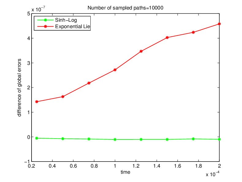
The error for the exponential Lie series integrator, we see in Figure 3, is larger than that for the stochastic Taylor integrator. The error for the sinh-log integrator is smaller, though only marginally so. In fact it is hardly discernible from the stochastic Taylor plot, so the middle panel shows a magnification of the left region of the plot in the top panel. We plot the differences between the errors in the lower panel to confirm the better performance of the sinh-log integrator over the global interval. Further, estimates for the local errors for the sinh-log and Lie series integrators from the data in Figure 3, of course, quantitatively match analytical estimates for the mean-square excess $E$ above.

Remark 5.3.

Generically the Castell–Gaines method of strong order one markedly outperforms the sinh-log method (which itself outperforms the stochastic Taylor method more markedly). However, as we have seen, there are pathological cases for which this is not true.

In Figure 4 we compare the global errors for the strong order three-halves sinh-log and stochastic Taylor methods, with governing linear vector fields with coefficient matrices

a_{1}=\begin{pmatrix}0&1\\ -1/2&-51/200\end{pmatrix}\qquad\text{and}\qquad a_{2}=\begin{pmatrix}1&1\\ 1&1/2\end{pmatrix}.

and initial data $y_{0}=(1,1/2)^{\text{\tiny T}}$ . Again as expected we see that the stochastic Taylor method is less accurate than the sinh-log method for sufficienltly small stepsizes.

Remark 5.4.

There is one caveat we have not mentioned thusfar. Constructing the approximation $\hat{\varphi}_{t}$ from $\hat{\psi}_{t}$ is in general nontrivial. For linear vector fields $V_{i}\circ y=a_{i}\,y$ , we know that $\hat{\psi}_{t}$ is simply a matrix, and we can straightforwardly construct $\hat{\varphi}_{t}$ using the matrix square root. For general nonlinear vector fields, we have not as yet found a superior method to simply expanding the square root shown to a sufficient number of high degree terms.

6 Concluding remarks

We have shown that the mean-square remainder associated with the sinh-log series is always smaller than the corresponding stochastic Taylor mean-square remainder, when there is no drift, to all orders. Since the order one-half sinh-log numerical method is the same as the order one-half Castell–Gaines method, it trivially inherits the asymptotically efficient property as well (indeed, if we include a drift term as well). We have not endeavoured to prove asymptotic efficiency more generally. However, in Section 5 we demonstrated that for two driving Wiener processes, the order one sinh-log numerical method is optimal in the following sense. From Figure 1, we see that any deviation of ${\epsilon}$ from zero will generate a negative eigenvalue for $b({\epsilon})$ . Consequently there exist vector fields such that the mean-square excess will be negative in regions of the phase space. Further, from Corollary 4.3, the order three-halves sinh-log integrator is also optimal in this sense. These results are only true when there is no drift, and it could be argued that our simulations and demonstrations are somewhat academic. However the results we proved have application in splitting methods for stochastic differential equations. For example, in stochastic volatility simulation in finance, Ninomiya & Victoir (2006) and Halley, Malham & Wiese (2008) simulate the Heston model for financial derivative pricing, and use splitting to preserve positivity for the volatility numerically. They employ a Strang splitting that separates the diffusion flow from the drift flow and requires a distinct simulation of the purely diffusion governed flow.

Why is the sinh-log expansion the answer? This result is intimately tied to the mean-square error measure we chose. The terms in the remainder of any truncation contain multiple Stratonovich integrals. Associated with each one is a mean-square error. There is a structure underlying these expectations. The sinh-log expansion somehow encodes this structure in an optimal form, it emulates the stochastic Taylor information more concisely. The next question is of course, what is the best structure when we include drift? Answering this is our next plan of action.

Acknowledgements.

We would like to thank Peter Friz, Terry Lyons and Hans Munthe–Kaas for interesting and useful discussions related to this work. We would also like to thank the anonymous referees for their critique and suggestions which helped improve the original manuscript.

References

[2] Azencott, R. 1982 Formule de Taylor stochastique et développement asymptotique d’intégrales de Feynman, Seminar on Probability XVI, Lecture Notes in Math. 921, Springer, 237–285
[4] Baudoin, F. 2004 An introduction to the geometry of stochastic flows Imperial College Press (2004)
[6] Ben Arous, G. 1989 Flots et series de Taylor stochastiques, Probab. Theory Related Fields 81, 29–77
[8] Burrage, K. & Burrage, P. M. 1999 High strong order methods for non-commutative stochastic ordinary differential equation systems and the Magnus formula, Phys. D 133, 34–48
[10] Castell, F. 1993 Asymptotic expansion of stochastic flows, Probab. Theory Related Fields 96, 225–239
[12] Castell, F. & Gaines, J. 1995 An efficient approximation method for stochastic differential equations by means of the exponential Lie series, Math. Comp. Simulation 38, 13–19
[14] Chen, K. T. 1957 Integration of paths, geometric invariants and a generalized Baker–Hausdorff formula, Annals of Mathematics 65(1), 163–178
[16] Connes, A. & Kreimer, D. 1998 Hopf algebras, renormalization and noncommutative geometry, Commun. Math. Phys. 199, 203–242
[18] Connes, A. & Miscovici, H. 1998 Cyclic cohomology and the transverse index theorem, Commun. Math. Phys. 198, 198–246
[20] Ebrahimi–Fard, K. & Guo, L. 2006 Mixable shuffles, quasi-shuffles and Hopf algebras, Journal of algebraic combinatorics 24(1), 83–101
[22] Fleiss, M. 1981 Functionelles causales non linéaires et indéterminées non-commutatives, Bulletin de la Société Mathématique de France 109, 3–40
[24] Gaines, J. 1994 The algebra of iterated stochastic integrals, Stochastics and Stochastics Reports 49, 169–179
[26] Halley, W., Malham, S.J.A. & Wiese, A. 2008 Positive stochastic volatility simulation, arXiv: 0802.4411.v1
[28] Iserles, A. 2002 Expansions that grow on trees, Notices of the AMS 49(4)
[30] Kawski, M. 2001 The combinatorics of nonlinear controllability and noncommuting flows, Lectures given at the Summer School on Mathematical Control Theory, Trieste
[32] Kloeden, P.E. & Platen, E. 1999 Numerical solution of stochastic differential equations, Springer
[34] Kunita, H., 1980 On the representation of solutions of stochastic differential equations, Lecture Notes in Math. 784, Springer–Verlag, 282–304
[36] Li, C.W. & Liu, X.Q. 2000 Almost sure convergence of the numerical discretization of stochastic jump diffusions, Acta. App. Math. 62, 225–244
[38] Lord, G., Malham, S.J.A. & Wiese, A. 2008 Efficient strong integrators for linear stochastic systems, SIAM J. Numer. Anal. 46(6), 2892–2919
[40] Lyons, T. 1998 Differential equations driven by rough signals, Rev. Mat. Iberoamericana 14(2), 215–310
[42] Lyons, T., Caruana, M. & Lévy, T. 2007 Differential equations driven by rough paths. École d’Été de Probabilités de Saint–Flour XXXIV-2004, Lecture Notes in Mathematics 1908, Springer
[44] Lyons, T. & Victoir, N. 2004 Cubature on Wiener space, Proc. R. Soc. Lond. A, 460, 169–198
[46] Magnus, W. 1954 On the exponential solution of differential equations for a linear operator, Comm. Pure Appl. Math. 7, 649–673
[48] Malham, S.J.A., Wiese, A. 2008 Stochastic Lie group integrators, SIAM J. Sci. Comput. 30(2), 597–617
[50] Manchon, D. & Paycha, S. 2007 Shuffle relations for regularised integrals of symbols, Communications in Mathematical Physics 270(1), 13–51
[52] Munthe–Kaas, H.Z. & Wright, W.M. 2007 On the Hopf algebraic structure of Lie group integrators, Foundations of Computational Mathematics 8(2), 227–257
[54] Murua, A. 2006 The Hopf algebra of rooted trees, free Lie algebras, and Lie series, Foundations of Computational Mathematics 6(4), 387–426
[56] Newton, N.J. 1991 Asymptotically efficient Runge–Kutta methods for a class of Îto and Stratonovich equations, SIAM J. Appl. Math. 51, 542–567
[58] Ninomiya, S. & Victoir, N. 2006 Weak approximation of stochastic differential equations and application to derivative pricing, arXiv:math/0605361v3
[60] Reutenauer, C. 1993 Free Lie algebras, London Mathematical Society Monographs New Series 7, Oxford Science Publications
[62] Strichartz, R.S. 1987 The Campbell–Baker–Hausdorff–Dynkin formula and solutions of differential equations, J. Funct. Anal. 72, 320–345
[64] Varadarajan, V. S. 1984 Lie groups, Lie algebras, and their representations, Springer
[66] Wiktorsson, M. 2001 Joint characteristic function and simultaneous simulation of iterated Itô integrals for multiple independent Brownian motions, Ann. Appl. Probab. 11(2), 470–487

	$\displaystyle\hat{\varphi}_{t_{0},t_{\ell}}$	$\displaystyle=\hat{\varphi}_{t_{m+1},t_{\ell}}\circ\biggl({\mathrm{id}}+\sum_{\|a\|=1}\tilde{K}_{a}(t_{m})V_{a}+\cdots\biggr)\circ\hat{\varphi}_{t_{0},t_{m}}$
		$\displaystyle={\mathrm{id}}+\sum_{\|a\|=1}\tilde{K}_{a}(t_{m})V_{a}+\cdots,$
and
	$\displaystyle\hat{\varphi}_{t_{m+1},t_{M}}$	$\displaystyle=\hat{\varphi}_{t_{\ell+1},t_{M}}\circ\biggl({\mathrm{id}}+\sum_{\|b\|=1}\tilde{K}_{b}(t_{\ell})V_{b}+\cdots\biggr)\circ\hat{\varphi}_{t_{m+1},t_{\ell}}$
		$\displaystyle={\mathrm{id}}+\sum_{\|b\|=1}\tilde{K}_{b}(t_{m})V_{b}+\cdots.$