Path Diversity over Packet Switched Networks:
Performance Analysis and Rate Allocation

From an end to end protocol’s perspective, performance of the lower layers in the protocol stack can be modeled as a random channel called the end-to-end channel. Since each packet usually includes an internal error detection coding (for instance a Cyclic Redundancy Check), the end-to-end channel is satisfactorily modeled as an erasure channel. Delay of the end-to-end channel is strongly dependent on its packet loss pattern, and affects the QoS considerably [48, 49].

In this work, the model assumed for the end-to-end channel is a two-state Markov model called Gilbert-Elliot cell, depicted in Fig. 1. The channel spends an exponentially distributed random amount of time with the mean $\frac{1}{\mu_{g}}$ in the Good state. Then, it alternates to the Bad state and stays in that state for another random duration exponentially distributed with the mean $\frac{1}{\mu_{b}}$. It is assumed that the channel state does not change during the transmission of a given packet [4, 50, 51]. Hence, if a packet is transmitted from the source at anytime during the good state, it will be received correctly. Otherwise, if it is transmitted during the bad state, it will eventually be lost before reaching the destination. Therefore, the average probability of error is equal to the steady state probability of being in the bad state, $\pi_{b}=\frac{\mu_{g}}{\mu_{g}+\mu_{b}}$. To have a reasonably low probability of error, $\mu_{g}$ must be much smaller than $\mu_{b}$. This model is widely used in the literature for theoretical analysis where delay is not a significant factor [1, 2, 3, 4, 5, 52, 50, 51]. Despite its simplicity, this model satisfactorily captures the bursty error characteristic of the end-to-end channel. More comprehensive models like the hidden Markov model are introduced in [49, 53]. Although analytically cumbersome, such models express the dependency of loss and delay more accurately.

A concatenated coding is used for packet transmission. The coding inside each packet can be a simple Cyclic Redundancy Check (CRC) which enables the receiver to detect an error inside each packet. Then, the receiver can consider the end-to-end channel as an erasure channel. Other than the coding inside each packet, a Forward Error Correction (FEC) scheme is applied between packets. Every $K$ packets are encoded to a Block of $N$ packets where $N>K$ to create some redundancy. The $N$ packets of each block are distributed across the $L$ available independent paths, and are received at the destination with some loss (erasure). The ratio of $\alpha=\frac{N-K}{N}$ defines the FEC overhead. A Maximum Distance Separable (MDS) $[N,K]$ code, such as the Reed-Solomon code, can reconstruct the original $K$ data packets at the receiver side if $K$ or more of the $N$ packets are received correctly [54]. According to the following theorem, an MDS code is the optimum block code we can design over any erasure channel. Although FEC imposes some bandwidth overhead, it might be the only option when feedback and retransmission are not feasible or fast enough to provide the desirable QoS.

Definition I. An erasure channel is defined as the one which maps every input symbol to either itself or to an erasure symbol $\xi$. More accurately, an arbitrary channel (memoryless or with memory) with the input vector $\mathbf{x}\in\mathcal{X}^{N}$, $|\mathcal{X}|=q$ , the output vector $\mathbf{y}\in\left(\mathcal{X}\cup\{\xi\}\right)^{N}$, and the transition probability $p\left(\mathbf{y}|\mathbf{x}\right)$ is defined to be erasure iff it satisfies the following conditions:

1. 1.

   $p\left(y_{j}\notin\left\{x_{j},\xi\right\}\right|x_{j})=0,~\forall~j$.

2. 2.

   Defining the erasure identifier vector $\mathbf{e}$ as

   $$e_{j}=\left\{\begin{array}[]{ll}1&y_{j}=\xi\\ 0&\mbox{otherwise}\end{array}\right.$$

   $p(\mathbf{e}|\mathbf{x})$ is independent of $\mathbf{x}$.

Theorem I. A block code of size $[N,K]$ with equiprobable codewords over an arbitrary erasure channel (memoryless or with memory) has the minimum probability of error (assuming optimum, i.e., maximum likelihood decoding) among all block codes of the same size if that code is Maximum Distance Separable (MDS). The proof is given in [6, 7].

The network is modeled as follows. $L$ independent paths, $1,2,\dots,L$, connect the source to the destination, as indicated in Fig. 2. Information bits are transmitted as packets, each of a constant length $r$. Furthermore, there is a constraint on the maximum rate for each path, meaning that the $i$’th path can support a maximum rate of $W_{i}$ packets per second. This constraint can be considered as an upperbound imposed by the physical characteristics of the path. As an example, [55] introduces the concept of the maximum TCP-friendly bandwidth for the maximum capacity of an Internet path. $W_{i}$’s are assumed to be known at the transmitter side. For a specific application and FEC scheme, we require a rate of $S_{req}$ packets per second from the source to the destination. Obviously, we should have $S_{req}\leq\sum_{i=1}^{L}W_{i}$ to have a feasible solution. The information packets are assumed to be coded in blocks of length $N$ packets. Hence, it takes $T=\frac{N}{S_{req}}$ seconds to transmit a block of packets. In practical scenarios with finite number of paths, the end-to-end required rate ($S_{req}$) is given, and the values of $N$ and $T$ have to be chosen based on the feasible complexity of the MDS decoder and the delay constraint of the application, respectively.

According to the FEC model, we can send $N_{i}$ packets through the path $i$ as long as $\sum_{i=1}^{L}N_{i}=N$ and $\frac{N_{i}}{T}\leq W_{i}$. The rate assigned to path $i$ can be expressed as $S_{i}=\frac{N_{i}}{T}=\frac{N_{i}}{N}S_{req}$, since the transmission instants of the $N_{i}$ packets are distributed evenly over the block duration $T$ (see Fig. 2). Obviously, we have $\sum_{i=1}^{L}S_{i}=S_{req}$. The objective of rate allocation problem is to find the optimal rate allocation vector or the vector $\mathbf{N}=(N_{1},\cdots,N_{L})$ which minimizes the probability of irrecoverable loss ($P_{E}$).

The above formulation of rate allocation problem is valid for any finite number of paths and any chosen values of $N$ and $T$. However, in section IV where the performance of path diversity is studied for a large number of paths, and also in Theorem III where the optimality of the proposed suboptimal algorithm is proved for the asymptotic case, we assume that $N$ grows linearly in terms of the number of paths, i.e. $N=n_{0}L$, for a fixed $n_{0}$. The reason behind this assumption is that when $L$ grows asymptotically large, the number of paths eventually exceeds the block length, if $N$ stays fixed. Thus, $L-N$ paths become useless for the values of $N$ larger than $N$. At the same time, it is assumed that the delay imposed by FEC, $T$, stays fixed with respect to $L$. This model results in a linearly increasing rate as the number of paths grows. We will later show that utilizing multiple paths, it is possible to simultaneously achieve an exponential decay in $P_{E}$ and a linear increase in rate, while the delay stays constant.

In this work, an irrecoverable loss is defined as the event where more than $N-K$ packets are lost in a block of $N$ packets. $P_{E}$ denotes the probability of this event. It should be noted that this probability is different from the decoding error probability of a maximum likelihood decoder performed on an MDS $[N,K]$ code, denoted by $\mathbb{P}\{\mathcal{E}\}$. Theoretically, an optimum maximum likelihood decoder of an MDS code may still decode the original codeword correctly with a positive, but very small probability, if it receives less than $K$ symbols (packets). More precisely, such a decoder is able to correctly decode an MDS code over $\mathbb{F}_{q}$ with the probability of $\frac{1}{q^{i}}$ after receiving $K-i$ correct symbols (see the proof of Theorem I in [6, 7] for more details). Of course, for Galois fields with a large cardinality, this probability is usually negligible. The relationship between $P_{E}$ and $\mathbb{P}\{\mathcal{E}\}$ can be summarized as follows:

Hence, $\mathbb{P}\{\mathcal{E}\}$ is bounded as

The reason $P_{E}$ is used as the measure of system performance is that while many practical low-complexity decoders for MDS codes work perfectly if the number of correctly received symbols is at least $K$, their probability of correct decoding is much less than that of maximum likelihood decoders when the number of correctly received symbols is less than $K$ [54]. Thus, in the rest of this paper, $P_{E}$ is used as a close approximation of decoding error.

To compute the probability of irrecoverable loss ($P_{E}$), we have to find the probability of $k_{i}$ packets being lost out of the $N_{i}$ packets transmitted through the path $i$, for $i$ from $1$ to $L$ and $k_{i}$ from $0$ to $N_{i}$. Let us denote the number of erroneous or lost packets over the path $i$ with the random variable $E_{i}$. Any two subsequent packets transmitted over the path $i$ are $\frac{1}{S_{i}}$ seconds apart in time, where $S_{i}$ is the transmission rate over the $i$’th path. We observe that the probability $\mathbb{P}\{E_{i}\geq k_{i}\}$ can be approximated with the continuous counterpart $\mathbb{P}\{B_{i}\geq\frac{k_{i}}{S_{i}}\}$ when the inter-packet interval is much shorter than the typical bad burst ($\frac{1}{S_{i}}\ll\frac{1}{\mu_{b}}$, or equivalently $\mu_{b}\ll S_{i}$). The necessity of this condition can be intuitively justified as follows. In case this condition does not hold, any two consecutive packets have to be transmitted on two independent states of the channel. Thus, no gain would be achieved by applying diversity over multiple independent paths. Figure 3 shows an example of this approximation in detail. The continuous approximation simplifies the mathematical analysis as discussed in section IV.

Probability of irrecoverable loss for one path is equal to

where $\mathbb{P}\{B>\alpha T|b\}$ and $\mathbb{P}\{B>\alpha T|g\}$ can be computed as

when the assumptions in section III and equations (4) and (7) are used. Thus, we have

where $(a)$ follows from the assumption that the end-to-end channel has a low probability of error ($\frac{1}{\mu_{g}}\gg\frac{1}{\mu_{b}}$).

As we observe, for large values of $\mu_{b}T$, $P_{E}$ decays exponentially with $\mu_{b}T$. Figure 4 shows the results of simulating a typical scenario of streaming data between two end-points with the rate $S_{req}=1000\frac{pkt}{sec}$, the block length $N=200$, and the number of information packets $K=180$. These values result in a block transmission time of $T=200ms$. The average good burst of the end-to-end channel, $\mu_{g}$, is selected such that $\mu_{g}T=\frac{1}{5}$. However, the average bad burst, $\mu_{b}$, varies such that $\mu_{b}T$ varies from $8$ to $40$, in accordance with the values in [3, 4]. The slope of the best linear fit (in semilog scale) to the simulation points is $0.097$ which is in accordance with the value of $0.100$, resulted from the theoretical approximation in (10).

When the paths are identical and have equal bandwidth constraints²² 2 The case where $W_{i}$’s are different is discussed in Remark V of subsection IV-C ($W_{i}=W$ for $\forall~1\leq i\leq L$), due to the symmetry of the problem, the uniform rate allocation ($\rho_{i}=\frac{1}{L}$) is obviously the optimum solution. Of course, the solution is feasible only when we have $\frac{1}{L}\leq\frac{W}{S_{req}}$. Then, the probability of irrecoverable loss can be simplified as

Let us define $Q(x)$ as the probability distribution function of $x$. Since $x$ is defined as $x=\frac{B}{T}$, clearly we have $Q(x)=Tf_{B}(xT)$. Defining $\mathbb{E}\{\}$ as the expected value operator throughout this paper, $\mathbb{E}\{x\}$ can be computed based on $Q(x)$. We observe that in (11), the random variable $x_{i}$’s are bounded and independent. Hence, the following well-known upperbound in large deviation theory [56] can be applied

where the $\log$ function is computed in Neperian base, and $\lambda$ is the solution of the following non-linear equation, which is shown to be unique by Lemma I.

Since $\lambda$ is unique, we can define $l(\alpha)=\lambda$. Even though being an upperbound, inequality (IV-B) is exponentially tight for large values of $L$ [56]. More precisely

where the notation $\doteq$ means $\displaystyle\lim_{L->\infty}-\frac{\log P_{E}}{L}=u(\alpha)$. Now, we state two useful lemmas whose proofs can be found in the appendices A and B.

Lemma I. $u(\alpha)$ and $l(\alpha)$ have the following properties:

1. 1.

   $\frac{\partial}{\partial\alpha}l(\alpha)>0$

2. 2.

   $l\left(\alpha=0\right)=-\infty$

3. 3.

   $l\left(\alpha=\mathbb{E}\{x\}\right)=0$

4. 4.

   $l\left(\alpha=1\right)=+\infty$

5. 5.

   $\frac{\partial}{\partial\alpha}u(\alpha)=l(\alpha)>0$ for $\alpha>\mathbb{E}\{x\}$

Lemma II. Defining $y=\frac{1}{L}\sum_{i=1}^{L}{x_{i}}$, where $x_{i}$’s are i.i.d. random variables as already defined, the probability density function of $y$ satisfies $f_{y}(\alpha)\doteq e^{-u(\alpha)L}$, for all $\alpha>\mathbb{E}\{x\}$.

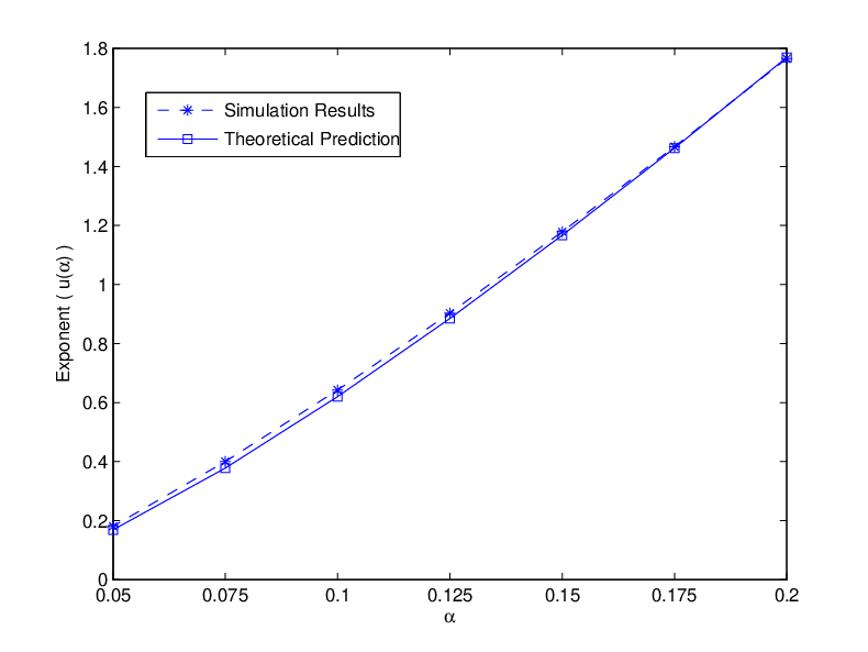
Figure 5 compares the theoretical and simulation results. We assume the block transmission time is $T=200ms$. The block length is proportional to the number of paths as $N=20L$. The average good burst of the end-to-end channel, $\mu_{g}$, is selected such that $\mu_{g}T=\frac{1}{5}$. The end-to-end channel has the error probability of $\pi_{b}=0.015$. Coding overhead is changed from $\alpha=0.05$ to $\alpha=0.2$. The probability of irrecoverable loss is plotted versus the number of paths, $L$, in semilogarithmic scale in Fig. 5 for different values of $\alpha$. We observe that as $L$ increases, $\log P_{E}$ decays linearly which is expected noting equation (IV-B). Also, Fig. 5 compares the slope of each plot in Fig. 5 with $u(\alpha)$. Figure 5 shows a good agreement between the theory and the simulation results, and also verifies the fact that the stronger the FEC code is (larger $\alpha$), the higher is the gain we achieve through path diversity (larger exponent).

Remark I. Equation (16) is a direct result of the discrete to continuous approximation in subsection III-A. Therefore, it remains valid even if the other approximations in section III do not hold. For example, if the block time contains more than one bad burst, equations (4) and (7) are no longer valid. However, equation (16) is still valid as long as the discrete to continuous approximation is used. Of course, in this case, the exact distributions of $B$ and $x$ should be used to compute $u(\alpha)$ and $\lambda$ instead of their simplified versions.

Remark II. A special case is when the block code uses all the bandwidth of the paths. In this case, we have $N=LWT$, where $W$ is the maximum bandwidth of each path, and $T$ is the block duration. Assuming $\alpha>\mathbb{E}\{x\}$ is a constant independent of $L$, we observe that the information packet rate is equal to $\frac{K}{T}=\left(1-\alpha\right)WL$, and the error probability is $P_{E}\doteq e^{-u\left(\alpha\right)L}$. This shows using MDS codes over multiple independent paths provides an exponential decay in the irrecoverable loss probability and a linearly growing end-to-end rate in terms of the number of paths, simultaneously.

Now, let us assume there are $J$ types of paths between the source and the destination, consisting of $L_{j}$ identical paths of type $j$ ($\sum_{j=1}^{J}{L_{j}}=L$). Without loss of generality, we assume that the paths are ordered according to their associated type, i.e. the paths from $1+\sum_{k=1}^{j-1}{L_{k}}$ to $\sum_{k=1}^{j}{L_{k}}$ are of type $j$. We denote $\gamma_{j}=\frac{L_{j}}{L}$. According to the i.i.d. assumption, it is obvious that $\rho_{i}$ has to be the same for all paths of the same type. $\eta_{j}$ and $y_{j}$ are defined as

Following Lemma II, we observe that $f_{y_{j}}(\beta_{j})\doteq e^{-\gamma_{j}u_{j}(\frac{\beta_{j}}{\eta_{j}})L}$. We define the sets $\mathcal{S}_{I}$, $\mathcal{S}_{O}$ and $\mathcal{S}_{T}$ as

respectively. Hence, $P_{E}$ can be written as

where $(a)$ follows from Lemma III, $(b)$ follows from the fact that $u_{j}(\alpha)$ is a strictly increasing function of $\alpha$, for $\alpha>\mathbb{E}\{x_{j}\}$, and $(c)$ can be proved as follows. Let us denote the vector which minimizes the exponent over the set $\mathcal{S}_{O}$ as $\hat{\boldsymbol{\beta}}^{\star}$. Since $\mathcal{S}_{T}$ is a subset of $\mathcal{S}_{O}$, $\hat{\boldsymbol{\beta}}^{\star}$ is either in $\mathcal{S}_{T}$ or in $\mathcal{S}_{O}-\mathcal{S}_{T}$. In the former case, $(c)$ is obviously valid. When $\hat{\boldsymbol{\beta}}^{\star}\in\mathcal{S}_{O}-\mathcal{S}_{T}$, we can prove that $0\leq\hat{\beta}_{j}^{\star}\leq\eta_{j}\mathbb{E}\{x_{j}\}$, for all $1\leq j\leq J$, by contradiction. Let us assume the opposite is true, i.e., there is at least one index $1\leq j\leq J$ such that $0\leq\hat{\beta}_{j}^{\star}\leq\eta_{j}\mathbb{E}\{x_{j}\}$, and at least one other index $1\leq k\leq J$ such that $\eta_{k}\mathbb{E}\{x_{k}\}<\hat{\beta}_{k}^{\star}$. Then, knowing that the derivative of of $u_{j}(\alpha)$ is zero for $\alpha=\mathbb{E}\{x_{j}\}$ and strictly positive for $\alpha>\mathbb{E}\{x_{j}\}$, a small increase in $\hat{\beta}_{j}^{\star}$ and an equal decrease in $\hat{\beta}_{k}^{\star}$ reduces the objective function, $\sum_{j=1}^{J}{\gamma_{j}u_{j}\left(\frac{\beta_{j}}{\eta_{j}}\right)}$, which contradicts the assumption that $\hat{\boldsymbol{\beta}}^{\star}$ is a minimum point. Knowing that $0\leq\hat{\beta}_{j}^{\star}<\eta_{j}\mathbb{E}\{x_{j}\}$, for all $1\leq j\leq J$, it is easy to show that the minimum value of the objective function is zero over $\mathcal{S}_{O}$, and $\mathcal{S}_{T}$ has to be an empty set. Defining the minimum value of the positive objective function as zero over an empty set ($\mathcal{S}_{T}$) makes $(c)$ valid for the latter case where $\hat{\boldsymbol{\beta}}^{\star}\in\mathcal{S}_{O}-\mathcal{S}_{T}$. Finally, applying Lemma IV results in $(d)$ where $\boldsymbol{\beta}^{\star}$ is defined in the Lemma.

Lemma III. For any continuous positive function $h(\mathbf{x})$ over a convex set $\mathcal{S}$, and defining $H(L)$ as

we have

where $cl(\mathcal{S})$ denotes the closure of $\mathcal{S}$ (refer to [57] for the definition of the closure operator). Proof of Lemma III can be found in appendix C.

Lemma IV. There exists a unique vector $\boldsymbol{\beta}^{\star}$ with the elements $\beta_{j}^{\star}=\eta_{j}l_{j}^{-1}\left(\frac{\nu\eta_{j}}{\gamma_{j}}\right)$ which minimizes the convex function $\sum_{j=1}^{J}{\gamma_{j}u_{j}(\frac{\beta_{j}}{\eta_{j}})}$ over the convex set $\mathcal{S}_{T}$, where $\nu$ satisfies the following condition

$l^{-1}()$ denotes the inverse of the function $l()$ defined in subsection IV-B. Proof of Lemma IV can be found in appendix D.

Equation (18) is valid for any fixed value of $\boldsymbol{\eta}$. To achieve the most rapid decay of $P_{E}$, the exponent must be maximized over $\boldsymbol{\eta}$.

where $\boldsymbol{\beta}^{\star}$ is defined for any value of the vector $\boldsymbol{\eta}$ in Lemma IV. Theorem II solves the maximization problem in (20) and identifies the asymptotically optimum rate allocation (for large number of paths).

Theorem II. Consider a point-to-point connection over the network with $L$ independent paths from the source to the destination, each modeled as a Gilbert-Elliot cell, with a large enough bandwidth constraint³³ 3 By the term ‘large enough’, we mean the bandwidth constraint on a path of type $j$, $W_{j}$, satisfies the condition $\frac{\eta_{j}n_{0}}{T\gamma_{j}}\leq W_{j}$. The reason is that $\eta_{j}$ must satisfy both conditions of $0\leq\eta_{j}\leq 1$ and $\frac{N_{j}}{TL_{j}}=\frac{\eta_{j}n_{0}L}{T\gamma_{j}L}\leq W_{j}$, simultaneously. When $W_{j}$ is large enough such that $\frac{\eta_{j}n_{0}}{T\gamma_{j}}\leq W_{j}$, the latter condition is automatically satisfied, and the optimization problem can be solved.. The paths are from $J$ different types, $L_{j}$ paths from the type $j$. Assume a block FEC of size $[N,K]$ is sent during a time interval $T$. Let $N_{j}$ denote the number of packets in a block of size $N$ assigned to the paths of type $j$, such that $\sum_{j=1}^{J}N_{j}=N$. The rate allocation vector $\boldsymbol{\eta}$ is defined as $\eta_{j}=\frac{N_{j}}{N}$. For fixed values of $\gamma_{j}=\frac{L_{j}}{L},~n_{0}=\frac{N}{L},~k_{0}=\frac{K}{L},~T$ and asymptotically large number of paths $L$, the optimum rate allocation vector $\boldsymbol{\eta}^{\star}$ can be found by solving the following optimization problem:

where $g(\boldsymbol{\eta})=\sum_{j=1}^{J}\gamma_{j}u_{j}\left(\frac{\beta_{j}^{\star}}{\eta_{j}}\right)$, and $\boldsymbol{\beta}^{\star}$ is an implicit function of $\boldsymbol{\eta}$ defined in Lemma IV. The functions $u_{j}()$ and $l_{j}()$ are defined in subsections IV-B and IV-C. Solving the above optimization problem gives the unique solution $\boldsymbol{\eta}^{\star}$ as

if there is at least one $1\leq j\leq J$ for which $\alpha>\mathbb{E}\{x_{j}\}$. Otherwise, when $\alpha\leq\mathbb{E}\{x_{j}\}$ for all $1\leq j\leq J$, the maximum value is zero for any arbitrary rate allocation vector, $\boldsymbol{\eta}$. In any case, the maximum value of the objective function is $g(\boldsymbol{\eta}^{\star})=\sum_{j=1}^{J}\gamma_{j}u_{j}(\alpha)$ which is indeed the exponent of $P_{E}$ versus $L$. The proof of the theorem can be found in appendix E.

Remark III. Theorem II can be interpreted as follows. For large values of $L$, adding a new type of path contributes to the path diversity iff the path satisfies the quality constraint $\alpha>\mathbb{E}\{x\}$, where $x$ is the percentage of time that the path spends in the bad state in the time interval $[0,T]$. Only in this case, adding the new type of path exponentially improves the performance of the system in terms of the probability of irrecoverable loss.

Remark IV. Observing the exponent coefficient corresponding to the optimum allocation vector $\boldsymbol{\eta}^{\star}$, we can see that the typical error event occurs when the ratio of the lost packets on all types of paths is the same as the total fraction of the lost packets, $\alpha$. However, this is not the case for any arbitrary rate allocation vector $\boldsymbol{\eta}$.

Remark V. An interesting extension of Theorem II is the case where all types have identical erasure patterns ($u_{j}(x)=u_{k}(x)$ for $\forall~1\leq j,k\leq J$ and $\forall x$), but different bandwidth constraints. Adopting the notation of Theorem II, the bandwidth constraint on $\eta_{j}$ can be written as $\frac{\eta_{j}n_{0}L}{T\gamma_{j}L}\leq W_{j}$, where $W_{j}$ is the maximum bandwidth for a path of type $j$. Let us define $\boldsymbol{\tilde{\eta}}^{\star}$ as the allocation vector which maximizes the objective function of Theorem II ($g(\boldsymbol{\eta})$), and satisfies the bandwidth constraints too. $\boldsymbol{\eta}^{\star}$ is also defined as the maximizing vector for the unconstrained problem in Theorem II. According to equation (21), we have $\eta^{\star}_{j}=\gamma_{j}$ for $\forall 1\leq j\leq J$. It is obvious that $\boldsymbol{\tilde{\eta}}^{\star}=\boldsymbol{\eta}^{\star}$ if $\eta^{\star}_{j}\leq\frac{\gamma_{j}W_{j}T}{n_{0}}$ for all $j$. In case $\eta^{\star}_{j}$ does not satisfy the bandwidth constraint for some $j$, $\boldsymbol{\tilde{\eta}}^{\star}$ can be found by the water-filling algorithm. More accurately, we have

where $\Upsilon$ can be found by imposing the condition $\sum_{j=1}^{J}\tilde{\eta}^{\star}_{j}=1$. Figure 7 depicts water-filling among identical paths with four different bandwidth constraints. Proof of equation (22) can be found in appendix F.

Figure 6 shows $P_{E}$ of the optimum rate allocation versus $L$ for a system consisting of two types of path. The optimal rate allocation is found by exhaustive search among all possible allocation vectors. The block transmission time is $T=200ms$. The block length is proportional to the number of paths as $N=20L$. The average good burst, $\mu_{g}$, is selected such that we have $\mu_{g}T=\frac{1}{5}$ for both types of paths. $\gamma_{1}=\frac{1}{3}$ of the paths (of the first type) benefit from shorter bad bursts and lower error probability of $\pi_{b,1}=0.015$, and the rest (the second type) suffer from longer congestion bursts resulting in a higher error probability of $\pi_{b,2}=0.025$. The coding overhead is $\alpha=0.1$. The figure depicts a linear behavior in semi-logarithmic scale with the exponent of $0.403$, which is comparable to $0.389$ resulted from (21).

In the scenario of Fig. 6, let us denote $\eta_{1}^{\star}$ as the value of of the first element of $\boldsymbol{\eta}$ in equation (21). Obviously, $\eta_{1}^{\star}$ does not depend on $L$. Moreover, $\eta_{1}^{opt}$ is defined as the normalized aggregated weight of type I paths in the optimal rate allocation. Figure 6 compares $\eta_{1}^{opt}$ with $\eta_{1}^{\star}$ for different number of paths. It is observed that $\eta_{1}^{opt}$ converges rapidly to $\eta_{1}^{\star}$ as $L$ grows. Figure 6 also verifies that the allocation vector candidate $\eta^{\star}$ proposed by Theorem II indeed meets the optimal allocation vector for large values of $L$.

References

- [1] J.C. Bolot, S. Fosse-Parisis, and D. Towsley, “Adaptive FEC-based error control for Internet telephony,” in IEEE INFOCOM, Proc. IEEE Vol. 3, 1999, pp. 1453–1460.
- [2] J.C. Bolot and T. Turletti, “Adaptive Error Control For Packet Video In The Internet,” in Proc. IEEE International Conference on Image Processing, 1996, pp. 25 – 28.
- [3] T. Nguyen and A. Zakhor , “Path diversity with forward error correction (pdf) system for packet switched networks,” in IEEE INFOCOM Proc. IEEE Vol. 1, 2003, pp. 663– 672.
- [4] T. Nguyen and A. Zakhor, “Multiple Sender Distributed Video Streaming,” IEEE transactions on multimedia, vol. 6, no. 2, pp. 315– 326, 2004.
- [5] F. L. Leannec, F. Toutain, and C. Guillemot, “Packet Loss Resilient MPEG-4 Compliant Video Coding for the Internet,” Journal of Image Communication, Special Issue on Real-time video over the Internet, no. 15, pp. 35–56, 1999.
- [6] S. Fashandi, S. Oveisgharan, and A.K. Khandani, “Coding over an Erasure Channel with a Large Alphabet Size,” in IEEE International Symposium on Information Theory, ISIT ’08, 2008.
- [7] ——, “Coding over an Erasure Channel with a Large Alphabet Size,” 2008, library and Archives Canada Technical Report UW-ECE #2008-06, http://cst.uwaterloo.ca/r/2008-06_Shervan.pdf.
- [8] H. Han, S. Shakkottai, C.V. Hollot, R. Srikant, and D. Towsley, “Multi-Path TCP: A Joint Congestion Control and Routing Scheme to Exploit Path Diversity in the Internet,” IEEE/ACM Transactions on Networking, vol. 14, no. 6, pp. 1260 – 1271, 2006.
- [9] S. Mao, S.S. Panwar, and Y.T. Hou, “On optimal partitioning of realtime traffic over multiple paths,” in INFOCOM 2005, Proc. IEEE Vol. 4, 2005, pp. 2325–2336.
- [10] S. Fashandi, S. Oveisgharan, and A.K. Khandani, “Path Diversity in Packet Switched Networks: Performance Analysis and Rate Allocation,” in IEEE Global Telecommunications Conference, GLOBECOM ’07, 2007, pp. 1840–1844.
- [11] J. Han, D. Watson, and F. Jahanian, “An Experimental Study of Internet Path Diversity,” IEEE Transactions on Dependable and Secure Computing, vol. 3, no. 4, pp. 273 – 288, 2006.
- [12] J. Han and F. Jahanian, “Impact of Path Diversity on Multi-homed and Overlay Networks,” in International Conference on Dependable Systems and Networks, 2004, pp. 29–38.
- [13] N. Spring, R. Mahajan, D. Wetherall, and T. Anderson, “Measuring ISP Topologies with Rocketfuel,” IEEE/ACM Transactions on Networking, vol. 12, no. 1, pp. 2– 16, 2004.
- [14] R. Teixeira, K. Marzullo, S. Savage, and G. M. Voelker, “In Search of Path Diversity in ISP Networks,” in Proceedings of the 3rd ACM SIGCOMM Conference on Internet Measurement, 2003, pp. 313 – 318.
- [15] A. L. Barbasi and R. Albert, “Emergence of Scaling in Random Networks,” Science, vol. 286, no. 5439, pp. 509–512, 1999.
- [16] David G. Andersen, Resilient Overlay Networks. Master’s Thesis, Massachusetts Institute of Technology, 2001.
- [17] Y. J. Liang, E. G. Steinbach, and B. Girod , “Multi-stream Voice over IP using Packet Path Diversity,” in IEEE Fourth Workshop on Multimedia Signal Processing, 2001, pp. 555–560.
- [18] S. Nelakuditi, Z. Zhang, and D. H. C. Du, “On Selection of Candidate Paths for Proportional Routing,” Elsevier Computer Networks, vol. 44, no. 1, pp. 79–102, 2004.
- [19] D. G. Andersen, A. C. Snoeren, and H. Balakrishnan, “Best-path vs. Multi-path Overlay Routing,” in Proceedings of the 3rd ACM SIGCOMM Conference on Internet Measurement, 2003, pp. 91 – 100.
- [20] B-G Chun, R. Fonseca, I. Stoica, and J. Kubiatowicz, “Characterizing Selfishly Constructed Overlay Routing Networks,” in IEEE INFOCOM, 2004, pp. 1329–1339.
- [21] J. Han, D. Watson, and F. Jahanian, “Topology Aware Overlay Networks,” in IEEE INFOCOM, vol. 4, 2005, pp. 2554– 2565.
- [22] M. Guo, Q. Zhang, and W. Zhu , “Selecting Path-diversified Servers in Content Distribution Networks,” in IEEE Global Telecommunications Conference, GLOBECOM ’03, vol. 6, 2003, pp. 3181–3185.
- [23] A. Akella, B. Maggs, S. Seshan, and A. Shaikh, “On the Performance Benefits of Multihoming Route Control,” IEEE/ACM Transactions on Networking, vol. 16, no. 1, pp. 91–104, 2008.
- [24] A. Akella, J. Pang, B. Maggs, S. Seshan, and A. Shaikh, “A Comparison of Overlay Routing and Multihoming Route Control,” in ACM SIGCOMM, 2004, pp. 93 – 106.
- [25] S. Srinivasan, Design and Use of Managed Overlay Networks. PhD Dissertation, Georgia Institute of Technology, 2007.
- [26] M. Cha, S. Moon, C. D. Park, and A. Shaikh, “Placing Relay Nodes for Intra-Domain Path Diversity,” in IEEE INFOCOM, 2006, pp. 1–12.
- [27] David Eppstein, “Finding the shortest paths,” in Proc. 35th Symp. Foundations of Computer Science, 1994, pp. 154–165.
- [28] Richard G. Ogier, Vlad Rutenburg, and Nauchum Shacham, “Distributed Algorithms for Computing Shortest Pairs of Disjoint Paths,” IEEE transactions on information theory, vol. 39, no. 2, pp. 443– 455, 1993.
- [29] D. Clark, W. Lehr, S. Bauer, P. Faratin, R. Sami, and J. Wroclawski, “Overlay Networks and Future of the Internet,” Journal of Communications and Strategies, vol. 3, no. 63, pp. 1–21, 2006.
- [30] M. Cha, Network Support for Emerging Multimedia Streaming Services. PhD Dissertation, Korea Advanced Institute of Science and Technology, 2007.
- [31] Roger Karrer, and Thomas Gross, “Multipath Streaming in Best-Effort Networks,” in Proc. of the IEEE International Conference on Communications (ICC’03), 2003.
- [32] J.G. Apostolopoulos, T. Wong, W. Tan, and S.J. Wee, “On Multiple Description Streaming with Content Delivery Networks,” in IEEE INFOCOM, Proc. IEEE Vol. 3, 2002, pp. 1736 – 1745.
- [33]
“Akamai SureRoute,”
http://www.akamai.com/dl/feature_sheets/fs_edge
suite_sureroute.pdf. - [34] M. Ghanassi and P. Kabal, “Optimizing Voice-over-IP Speech Quality Using Path Diversity,” in IEEE 8th Workshop on Multimedia Signal Processing, 2006, pp. 155–160.
- [35] J. Chakareski and B. Girod, “Rate-distortion optimized packet scheduling and routing for media streaming with path diversity,” in Proc. IEEE Data Compression Conference, 2003, pp. 203– 212.
- [36] M. Afergan, J. Wein, and A. LaMeyer, “Experience with some Principles for Building an Internet-Scale Reliable System,” in Proceedings of the Fifth IEEE International Symposium on Network Computing and Applications (NCA’06), 2006, p. 3.
- [37] Ron M. Roth, Introduction to Coding Theory, 1st ed. Cambridge University Press, 2006, pp. 333–351.
- [38] W. T. Tan and A. Zakhor, “Video Multicast Using Layered FEC and Scalable Compression,” IEEE Transactions on Circuits and Systems for Video Technology, vol. 11, no. 3, pp. 373–386, 2001.
- [39] L. Dairaine, L. Lancérica, J. Lacan, and J. Fimes, “Content-Access QoS in Peer-to-Peer Networks Using a Fast MDS Erasure Code,” Elsevier Computer Communications, vol. 28, no. 15, pp. 1778–1790, 2005.
- [40] X. H. Peng, “Erasure-control Coding for Distributed Networks,” IEE Proceedings on Communications, vol. 152, pp. 1075 – 1080, 2005.
- [41] N. Alon, J. Edmonds, and M. Luby, “Linear Time Erasure Codes with Nearly Optimal Recovery,” in IEEE Symposium on Foundations of Computer Science, Proc. IEEE Vol. 3, 1995, pp. 512–519.
- [42] J. Justesen , “On the complexity of decoding Reed-Solomon codes,” IEEE transactions on information theory, vol. 22, no. 2, pp. 237– 238, 1993.
- [43] M. G. Luby, M. Mitzenmacher, M. A. Shokrollahi, and D. A. Spielman, “Efficient Erasure Correcting Codes,” IEEE Transactions on Information Theory, vol. 47, no. 2, pp. 569–584, 2001.
- [44] A. Shokrollahi, “Raptor Codes,” IEEE Transactions on Information Theory, vol. 52, no. 6, pp. 2551–2567, 2006.
- [45] R. Koetter and M. Medard , “An algebraic approach to network coding,” IEEE transactions on Networking, vol. 11, no. 5, pp. 782– 795, 2003.
- [46] P. A. Chou, Y. Wu, and K. Jain, “Practical Network Coding ,” in 51st Allerton Conference on Communication, Control and Computing, 2003.
- [47] C. Gkantsidis and P. R. Rodriguez, “Network coding for large scale content distribution,” in IEEE INFOCOM, Proc. IEEE Vol. 4, 2005, pp. 2235–2245.
- [48] M. Yajnik, S.B. Moon, J.F. Kurose, and D.F. Towsley , “Measurement and Modeling of the Temporal Dependence in Packet Loss,” in IEEE INFOCOM Proc. IEEE Vol. 1, 1999, pp. 345–352.
- [49] P. Rossi, G. Romano, F. Palmieri, and G. Iannello , “A Hidden Markov Model for Internet Channels,” in IEEE International Symposium on Signal Processing and Information Technology, 2003.
- [50] W. Kellerer, E. Steinbach, P. Eisert, and B. Girod, “A Real-Time Internet Streaming Media Testbed,” in Proc. IEEE International Conference on Multimedia and Expo, 2002, pp. 453– 456.
- [51] X. Henocq and C. Guillemot, “Source Adaptive Error Control for Real-time Video over the Internet,” Numéro spécial image et vidéo. Hermès. Réseaux et système réparti. Calculateurs Parallèles, vol. 12, no. 3-4, 2000.
- [52] F. L. Leannec and C. Guillemot, “Error Resilient Video Transmission over the Internet,” in Proc. Visual Communication and Image Processing, 1999.
- [53] K. Salamatian and Vaton, “Hidden Markov Modeling for Network Communication Channels,” in Proc. ACM SIGMETRICS, 2001, pp. 92 – 101.
- [54] Ron M. Roth, Introduction to Coding Theory, 1st ed. Cambridge University Press, 2006, pp. 183–204.
- [55] J. Padhye, V. Firoiu, D.F Towsley, and J.F. Kurose, “Modeling TCP Reno performance: a simple model and its empirical validation,” IEEE/ACM Transactions on Networking, vol. 8, no. 2, pp. 133 – 145, 2000.
- [56] Amir Dembo and Ofer Zeitouni, Large Deviations Techniques and Applications, 2nd ed. New York: Springer, 1998, pp. 11–43.
- [57] J. L. Kelley, General Topology. Springer, 1975, pp. 40–43.
- [58] C. H. Papadimitriou, Computational Complexity, 1st ed. New York: Addison Wesley, 1994.
- [59] T. H. Cormen, C. E. Leiserson, R. L. Rivest, and C. Stein, Introduction to Algorithms, 2nd ed. MIT Press, 2001, pp. 347–349.
- [60] W. Rudin, Principles of Mathematical Analysis, 3rd ed. McGraw-Hill, 1976.
- [61] S. Boyd and L. Vandenberghe, Convex Optimization, 1st ed. Cambridge, UK: Cambridge University Press, 2004, pp. 243–245.
- [62] T. Cover and J. Thomas, Elements of Information Theory, 1st ed. New York: Wiley, 1991, pp. 291–294.
- [63] ——, Elements of Information Theory, 1st ed. New York: Wiley, 1991, pp. 30–31.