Constructing the Simplest Possible Phylogenetic Network from TripletsThanks: Part of this research has been funded by the Dutch BSIK/BRICKS project.
Abstract
A phylogenetic network is a directed acyclic graph that visualises an evolutionary history containing so-called reticulations such as recombinations, hybridisations or lateral gene transfers. Here we consider the construction of a simplest possible phylogenetic network consistent with an input set , where contains at least one phylogenetic tree on three leaves (a triplet) for each combination of three taxa. To quantify the complexity of a network we consider both the total number of reticulations and the number of reticulations per biconnected component, called the level of the network. We give polynomial-time algorithms for constructing a level-1 respectively a level-2 network that contains a minimum number of reticulations and is consistent with (if such a network exists). In addition, we show that if is precisely equal to the set of triplets consistent with some network, then we can construct such a network with smallest possible level in time , if is a fixed upper bound on the level of the network.
1 Introduction
One of the ultimate goals in computational biology is to create methods that can reconstruct evolutionary histories
from biological data of currently living organisms. The immense complexity of biological evolution makes this task
almost a hopeless one [20]. This has motivated researchers to focus first on the simplest possible pattern
of evolution. This least complicated shape of an evolutionary history is the tree-shape. Now that treelike evolution has
been extremely well studied, a logical next step is to consider slightly more complicated evolutionary scenarios,
gradually extending the complexity that our models can describe. At the same time we also wish to take into account the
parsimony principle, which tells us that amongst all equally good explanations of our data, one prefers the simplest one
(see e.g. [11]).
For a set of taxa (e.g. species or strains), a phylogenetic tree describes (a hypothesis of) the evolution that these
taxa have undergone. The taxa form the leaves of the tree while the internal vertices represent events of genetic
divergence: one incoming branch splits into two (or more) outgoing branches.
Phylogenetic networks form an extension to this model where it is also possible that two branches combine into one new
branch. We call such an event a reticulation, which can model any kind of non-treelike (also called
“reticulate”) evolutionary process such as recombination, hybridisation or lateral gene transfer. In addition,
reticulations can also be used to display different possible (treelike) evolutions in one figure. In recent years
there has emerged enormous interest in phylogenetic networks and their application
[3][12][18][20][21].
This model of a phylogenetic network allows for many different degrees of complexity, ranging from networks that are
equal, or almost equal, to a tree to unrealistically complex webs of frequently diverging and recombining lineages.
Therefore we consider two different measures for the complexity of a network. The first of these measures is the total
number of reticulations in the network. Secondly, we consider the level of the network, which is an upper bound
on the number of reticulations per biconnected component of the network. Informally, the level of a network is a bound
on the number of reticulations that can be mutually dependent. In this paper we consider two different approaches for
constructing networks that are as simple as possible. The first approach minimises the total number of reticulations
for a fixed level (of at most two) and the second approach minimises (under certain special restrictions on the input)
the level while the total number of reticulations is unrestricted.
Level- phylogenetic networks were first introduced by Choy et al. [7] and further studied by different
authors [14][15][17]. Gusfield et al. gave a biological justification for level-1
networks (which they call “galled trees”) [9]. Minimising reticulations has been very well studied in
the framework where the input consists of (binary) sequences [10][11][23][24]. For
example, Wang et al. considered the problem of finding a “perfect phylogeny” with a minimum number of reticulations
and showed that this problem is NP-hard [25]. Gusfield et al. showed that this problem can be solved in
polynomial time if restricted to level-1 networks [9].
There are also several results known already about the version of the problem where the input consists of a set of
trees and the objective is to construct a network that is “consistent” with each of the input trees. Baroni et al.
give bounds on the minimum number or reticulations needed to combine two trees [2] and Bordewich et al.
showed that it is APX-hard to compute this minimum number exactly [4]. However, there exists an exact
algorithm [5] that runs reasonably fast in many practical situations.
In this paper we also consider input sets consisting of trees, but restrict ourselves to small trees with three leaves
each, called triplets. See Figure 1 for an example. Triplets can for example be
constructed by existing methods, such as Maximum Parsimony or Maximum Likelihood, that work accurately and fast for
small numbers of taxa. Triplet-based methods have also been well-studied. Aho et al. [1] gave a polynomial-time
algorithm to construct a tree from triplets if there exists a tree that is consistent with all input triplets. Jansson
et al. [16] showed that the same is possible for level-1 networks if the input triplet set is dense, i.e.
if there is a triplet for any set of three taxa. Van Iersel et al. further extended this result to level-2 networks
[14]. From non-dense triplet sets it is NP-hard to construct level- networks for any
[15][16]. From the proof of this result also follows directly that it is NP-hard to find a network
consistent with a non-dense triplet set that contains a minimum number of reticulations.11
1
This follows from
the proof of Theorem 7 in [16], since only one reticulation is used in their reduction. It is unknown whether
this problem becomes easier if the input triplet set is dense.

In the first part of this paper we consider fixed-level networks and aim to minimise the total number of
reticulations in these networks. In Section 3 we give a polynomial-time algorithm that constructs a
level-1 network consistent with a dense triplet set (if such a network exists) and minimises the total number of
reticulations over all such networks. This gives an extension to the algorithm by Jansson et al. [16], which can
also reconstruct level-1 networks, but does not minimise the number of reticulations. To illustrate this we give in
Section 2 an example dense triplet set on leaves for which the algorithm in [16] (and the
ones in [14] and [17]) creates a level-1 network with reticulations. However, a level-1
network with just one reticulation is also possible and our algorithm MARLON is able to find that network. We have
implemented MARLON (made publicly available [19]) and tested it on simulated data. Results are in
Section 4. The worst case running time of the algorithm is for leaves (and hence
with the input size).
In Section 5 we further extend this approach by giving an algorithm that even constructs a level-2
network consistent with a dense triplet set (if one exists) and again minimises the total number of reticulations over
all such networks. This means that if the level is at most two, we can minimise both the level and the total number of
reticulations, giving priority to the criterium that we find most important. The running time is (and
thus ).
Minimising the level of phylogenetic networks becomes even more challenging when this level can be larger than two,
even without minimising the total number of reticulations. Given a dense set of triplets, it is a major open problem
whether one can construct a minimum level phylogenetic network consistent with these triplets in polynomial time.
Moreover, it is not even known whether it is possible to construct a level-3 network consistent with a dense input
triplet set in polynomial time. In Section 6 of this paper we show some significant progress in this
direction. As a first step we consider the restriction to “simple” networks, i.e. networks that contain just one
nontrivial biconnected component. We show how to construct, in time, a minimum level simple network
with level at most from a dense input triplet set (for fixed ). Subsequently we show that this can be used to
also generate general level- networks if we put an extra restriction on the quality of the input triplets. Namely,
we assume that the input set contains exactly all triplets consistent with some network. If that is the case then our
algorithm can find such a network with a smallest possible level. The algorithm runs in polynomial time
if the upper bound on the level of the network is fixed. This result constitutes an important step forward in the
analysis of level- networks, since it provides the first positive result that can be used for all levels .
2 Preliminaries
A phylogenetic network (network for short) is defined as a directed acyclic graph in which exactly one
vertex has indegree 0 and outdegree 2 (the root) and all other vertices have either indegree 1 and outdegree 2
(split vertices), indegree 2 and outdegree 1 (reticulation vertices, or reticulations for short)
or indegree 1 and outdegree 0 (leaves), where the leaves are distinctly labelled. A phylogenetic network
without reticulations is called a phylogenetic tree.
A directed acyclic graph is connected (also called “weakly connected”) if there is an undirected
path between any two vertices and biconnected if it contains no vertex whose removal disconnects the graph. A
biconnected component of a network is a maximal biconnected subgraph and is called trivial if
it is equal to two vertices connected by an arc. To avoid “redundant” networks we assume that in any network
every nontrival biconnected component has at least three outgoing arcs. We call an arc of a network
a cut-arc if its removal disconnects and call it trivial if is a leaf.
Definition 1
A network is said to be a level- network if each biconnected component contains at most reticulations.
A level- network that contains no nontrivial cut-arcs and is not a level- network is called a simple
level- network22
2
This definition is equivalent to Definition 4 in [14] by Lemma 2 in
[14].. Informally, a simple network thus consists of a nontrivial biconnected component with leaves
“hanging” of it.
A triplet is a phylogenetic tree on the leaves , and such that the lowest common ancestor of
and is a proper descendant of the lowest common ancestor of and . The triplet is displayed in
Figure 1. Denote the set of leaves in a network by . For any set of triplets define
and let . A set of triplets is called dense if for each at least one of , and belongs to .
For a set of triplets and a set of leaves , we denote by the triplets with . Furthermore, if is a collection of leaf-sets we use
to denote the induced set of triplets such that there exist ,
, with and , and all distinct.
Definition 2
A triplet is consistent with a network (interchangeably: is consistent with ) if contains a subdivision of , i.e. if contains vertices and pairwise internally vertex-disjoint paths , , and .
The above definitions enable us to give a formal description of the problems we consider.
Problem: Minimum Reticulation Level- network on dense triplet sets (DMRL-).
Input: dense set of triplets .
Output: level- network that is consistent with (if such a network exists) and has a minimum number
of reticulations over all such networks.
A feasible solution to DMRL-1 can be found by the algorithm in [16] or [17] and the algorithm in
[14] finds a feasible solution to DMRL-2. To show that these algorithms do not always minimise the number of
reticulations, consider a triplet set over an odd number of leaves, labelled , containing all triplets
with and the triplets with . The aforementioned algorithms find for this
input set a level-1 network with reticulations. However, a level-1 network with just one reticulation
is also possible and our algorithm MARLON, introduced shortly, is able to find that network. See Figure 2 for an example
for .


Given a network let denote the set of all triplets consistent with . We say that a
network reflects a triplet set if . If, for a triplet set , there exists a network
that reflects it, we say that is reflective. The second problem we consider is thus the following:
Problem: MIN-REFLECT-
Input: set of triplets .
Output: level- network that reflects (if such a network exists) and has the smallest possible
level over all such networks.
Note that this problem is closely related to the mixed triplets problem (MT) studied in [forbid], which
asks for a phylogenetic network consistent with an input triplet set and not consistent with another input
triplet set . Namely, MIN-REFLECT- is a special case of MT restricted to level- networks where the set of
forbidden triplets contains all triplets that are not in .
To describe our algorithms we need to introduce some more definitions. We say that a cut-arc is a
highest cut-arc if it is not reachable from any other cut-arc. We call a cycle containing the root a
highest cycle and a reticulation in such a cycle a highest reticulation. We say that a leaf is
below an arc (and below vertex ) if is reachable from . In the next section we will
frequently use the set , which denotes the set of leaves in network that is below a highest
reticulation.
A subset of the leaves is an SN-set (w.r.t. triplet set ) if there is no triplet in with
, . An SN-set is called nontrivial if it does not contain all leaves. We say that an
SN-set is maximal (under restriction ) if there is no nontrivial SN-set (satisfying restriction )
that is a strict superset of . An SN-set of size 1 is called a singleton SN-set.
Any two SN-sets w.r.t. a dense triplet set are either disjoint or one is included in the other [17, Lemma 8],
which leads to the following definition. The SN-tree is a directed tree with vertices with outdegree greater or
equal to two, such that the SN-sets of correspond exactly to the sets of leaves reachable from a vertex of the
SN-tree. It follows that there are at most nontrivial SN-sets in a dense triplet set . All these SN-sets
can be found by constructing the SN-tree in time [16]. If a network is consistent with a dense triplet
set , then the set of leaves below any cut-arc is always an SN-set, since triplets of the form with
, , are not consistent with such a network. Furthermore, each maximal SN-set is equal to the
union of leaves below one or more highest cut-arcs [13, Lemma 5].
3 Constructing a Level-1 Network with a Minimum Number of Reticulations
We propose the following dynamic programming algorithm for solving DMRL-1. The algorithm considers all SN-sets from
small to large and computes an optimal solution for each SN-set , based on the optimal solutions for included
SN-sets. The algorithm considers both the case where the root of is contained in a cycle and the case where
there are two cut-arcs leaving the root. In the latter case there are two SN-sets and that are maximal
under the restriction that they are a subset of . If this is the case then the algorithm constructs a candidate for
by creating a root connected to the roots of and .
The other possibility is that the root of is contained in some cycle. For this case the algorithm tries each
SN-set as : the set of leaves below the highest reticulation. The sets of leaves below other highest
cut-arcs can then be found using the property of optimal level-1 networks outlined in Lemma 1.
Subsequently, an induced set of triplets is computed, where each set of leaves below a highest cut-arc is replaced by
a single meta-leaf. A candidate network is constructed by computing a simple level-1 network and replacing each
meta-leaf by an optimal network for the corresponding subset of the leaves. The optimal network
is then the network with a minimum number of reticulations over all computed networks.
A structured description of the computations is in Algorithm 1. We use to denote the minimum
number of reticulations in any level-1 network consistent with . In addition, denotes the minimum
number of reticulations in any level-1 network consistent with with . The algorithm first computes
the optimal number of reticulations. Then a network with this number of reticulations is constructed using
backtracking.
To show that the algorithm indeed computes an optimal solution we need the following crucial property of optimal level-1 networks.
Lemma 1
If there exists a solution to DMRL-1, then there also exists an optimal solution , where the sets of leaves below highest cut-arcs equal either (i) and the SN-sets that are maximal under the restriction that they do not contain , or (ii) the maximal SN-sets (if ).
Proof
If then there are two highest cut-arcs and the sets below them are the maximal SN-sets. Otherwise, the root of is part of a cycle. Let be a maximal SN-set. We prove the following.
Claim (1)
Maximal SN-set equals either the set of leaves below a highest cut-arc or the set of leaves below a directed path ending in the highest reticulation or in one of its parents.
Proof
If equals the set of leaves below a single highest cut-arc then we are done. From now on assume that equals the set of leaves below different highest cut-arcs. First observe that no two leaves in have the root as their lowest common ancestor, since this would imply that all leaves are in , because is an SN-set. From this follows that all leaves in are below some directed path on the highest cycle. First assume that not all leaves reachable from vertices in are in . Then there are leaves reachable respectively from vertices that are on (in this order) with and . But this leads to a contradiction because then the triplet is not consistent with , whilst and cannot be in since is an SN-set. It remains to prove that ends in either the highest reticulation or in one of its parents. Assume that this is not true, then there exists a vertex on (the interior of) a path from the last vertex of to the highest reticulation. Consider some leaf reachable from and some leaves below different highest cut-arcs. Then this again leads to a contradiction because is not consistent with . This concludes the proof of the claim. ∎
First suppose that a maximal SN-set equals the set of leaves below a directed path ending in a parent of the
highest reticulation. In this case we can modify the network by putting below a single cut-arc, without increasing
the number of reticulations. To be precise, if and are the first and last vertex of respectively and
is the highest reticulation, then we subdivide the arc entering by a new vertex , add a new arc , remove
the arc and suppress the resulting vertex with indegree and outdegree both equal to one. It is not too
difficult to see that the resulting network is still consistent with .

Now suppose that some maximal SN-set equals the set of leaves below a directed path ending in the
highest reticulation. The sets of leaves below highest cut-arcs are all SN-sets (as is always the case). One of them
is equal to . If any of the others is contained in a nontrivial SN-set that does not contain ,
then the procedure from the previous paragraph can again be used to put below a highest cut-arc. In the resulting
network the sets of leaves below highest cut-arcs are indeed equal to and the SN-sets that
are maximal under the restriction that they do not contain .
An example is given in Figure 3. In the network on the left one maximal SN-set equals the set of leaves
below the red path. In the middle is the same network, but now we encircled and the SN-sets that are maximal
under the restriction that they do not contain . There is still an SN-set () below a path on the cycle
(again in red). However, in this case the network can be modified by putting below a single cut-arc, without
increasing the number of reticulations. This gives the network to the right, where the sets of leaves below highest
cut-arcs are indeed equal to and the SN-sets that are maximal under the restriction that they do not contain
.∎
Theorem 3.1
Given a dense set of triplets , algorithm MARLON constructs a level-1 network that is consistent with (if such a network exists) and has a minimum number of reticulations in time.
Proof
The proof is by induction on the size of . Suppose that is an optimal level-1 network consistent with . If then the sets of leaves below highest cut-arcs are the two maximal SN-sets and . In this case can be computed by adding up the and . Otherwise, it follows from Lemma 1 and the observation that has to be an SN-set, that at some iteration the algorithm will consider the set equal to the sets of leaves below the highest cut-arcs of . In this case the number of reticulations can be computed by adding one to the sum of the values over all . This is because the network consists of a (highest) cycle, connected to optimal networks for the different . By induction, all values of for have been computed correctly and correctness of the algorithm follows. The number of SN-sets is because any two SN-sets are either disjoint or one is included in the other [17, Lemma 8]. These SN-sets can be found in time by computing the SN-tree [16]. Simple level-1 networks can be found in time [16] and can be computed in time. These computations are repeated times: for all and all with . Therefore, the total running time is . ∎
4 Experiments
MARLON has been implemented, tested and made publicly available [19]. For example the network in
Figure 4 with 80 leaves and 13 reticulations could be constructed by MARLON in less than six minutes on
a Pentium IV 3 GHz PC with 1 GB of
RAM.

To test the relevance of the constructed networks we applied MARLON to simulated data. The main advantage of
using simulated data is that it enables us to compare output networks with the “real” network. We repeated the
following experiment for different level-1 networks, which we in turn assumed to be the “real” network. Given such a
level-1 network, we used the program Seq-Gen [22] to simulate sequences that could have evolved according to
that network. We simulated a recombinant phylogeny by generating sequences of 4000 base pairs, consisting of two
blocks of 2000 base pairs each. We assumed that each block evolved according to a phylogenetic tree. This means that
in each simulation, our input to Seq-Gen consisted of two trees and . For each reticulation of the level-1
network, uses just one of the incoming arcs and uses the other one. This makes sure that each arc of the
network is used by at least one of the two trees. Seq-Gen was used with the F81 model of nucleotide
substitution.


From these simulated sequences we computed a set of triplets as follows. We assume that for one sequence it
is known that it is only distantly related to the others. This is called the outgroup sequence. For each
combination of three sequences, plus the outgroup sequence, we computed a phylogenetic tree using the maximum
likelihood method PHYML
[8]. The output trees of PHYML give a dense triplet set, which we used as input to MARLON.
All simulations gave similar results. Here we describe the results for one specific “real” level-1
network, displayed in Figure 5. We obtained the simulated triplet set based on this network by
the procedure described above. For this triplet set MARLON constructed the output network in
Figure 6. The constructed network is very similar to the input network (which we assumed to be the
“real” network). Both networks have four reticulations and also the branching structure is almost identical. The
only differences are all of the following type. The output network contains some subnetworks rooted below a parent of
a reticulation. In some of these cases the input network is a bit different because here the subnetwork is divided
below a path on the cycle, ending in the parent of the reticulation. For example in Figure 5 the
leaves 37, 38, 39, 40 are below a path on a cycle consisting of three vertices. However, in the output network in
Figure 6 these leaves are below a single vertex on the cycle.
Other simulations give similar results. The networks constructed by MARLON are almost identical to the input
networks, except for some small differences that are almost all of the type described above. In one case the output
network also contained an extra reticulation that was not present in the input network. In this case there must have
been triplets in the simulated triplet set that were not consistent with the input network.
We conclude that MARLON correctly constructs level-1 networks and works very fast. For simulated data the produced
networks are very close to the “real” networks used to generate the simulated sequences. When using real data we
expect the amount of incorrect triplets to be larger and hence the results possibly less impressive. In addition, real
data sets will not always originate from a level-1 network, in which case MARLON will not be able to compute a
solution. This problem will partly be solved in the next section where we show how the approach can be extended to
level-2. However, the main conclusion to be drawn from the experiments is that, if the data is good enough, our method
is indeed able to produce good estimates of evolutionary histories. This for example shows that, when a set of
triplets is computed from sequence data, sufficient information is retained to be able to reconstruct the phylogenetic
network accurately. In addition, MARLON provides a very fast method to combine these triplets into a phylogenetic
network.
5 Constructing a Level-2 Network with a Minimum Number of Reticulations
This section extends the approach from Section 3 to level-2 networks. We describe how one can find a
level-2 network consistent with a dense input triplet set containing a minimum number of reticulations, or decide that
such a network does not exist.
The general structure of the algorithm is the same as in the level-1 case. We loop though all SN-sets from small
to large and compute an optimal solution for that SN-set, based on previously computed optimal solutions for
included SN-sets. For each SN-set we still consider, like in the level-1 case, the possibility that there are two
cut-arcs leaving the root of and the possibility that this root is in a biconnected component with one
reticulation. However, now we also consider a third possibility, that the root of is in a biconnected component
containing two reticulations.
In the construction of biconnected components with two reticulations, we use the notion of
“non-cycle-reachable”-arc, or n.c.r.-arc for short, introduced in [15]. We call an arc an
n.c.r.-arc if is not reachable from any vertex in a cycle. These n.c.r.-arcs will be used to combine
networks without increasing the network level. In addition, we use the notion highest biconnected
component to denote the biconnected component containing the root.

Our complete algorithm is described in detail in Algorithm 2. To get an intuition of why the
algorithm works, consider the four possible structures of a biconnected component containing two reticulations
displayed in Figure 7. Let , , and be the sets of leaves indicated in
Figure 7 in the graph that displays the form of the highest biconnected component of . Observe
that after removing in each case , and become a set of leaves below a cut-arc and hence an SN-set
(w.r.t ). In cases 2a, 2b and 2c the highest biconnected component becomes a cycle, the set of
leaves below the highest reticulation and and sets of leaves below highest cut-arcs. We will first
describe the approach for these cases and show later how a similar technique is possible for case 2d.
Our algorithm loops through all SN-sets that are a subset of and will hence at some iteration consider the SN-set
. The algorithm removes the set and computes the SN-sets w.r.t. . The sets of leaves below
highest cut-arcs (in some optimal solution, if one exists) are now equal to and the SN-sets that are maximal
under the restriction that they do not contain , or (by the same arguments as in the proof of
Lemma 1). Therefore, the algorithm tries each possible SN-set for , and and in one of these
iterations it will correctly determine the sets of leaves below highest cut-arcs. Then the algorithm computes the
induced set of triplets, where each set of leaves below a highest cut-arc is replaced by a single meta-leaf. All
simple level-1 networks consistent with this induced set of triplets are obtained by the algorithm in [16]. Our
algorithm loops through all these networks and does the following for each simple level-1 network . Each
meta-leaf , not equal to or , is replaced by an optimal network , which has been computed in a previous
iteration. To include leaves in , and , we compute an optimal network consistent with and an
optimal network consistent with where in both networks is the set of leaves below an n.c.r.-arc. Then
we combine these three networks into a single network like in Figure 8. A new reticulation is
created and becomes the set of leaves below this reticulation. Finally, we check for each constructed network
whether it is consistent with . The network with the minimum number of reticulations over all
such networks is the optimal solution for this SN-set.
Now consider case 2d. Suppose we remove and replace , (=) and each SN-set w.r.t. that
is maximal under the restriction that it does not contain or by a single leaf. Then the resulting network
consists of a path ending in a simple level-1 network, with a child of the root and the child of the
reticulation; and each vertex of the path has a leaf as child. Such a network can easily be constructed and
subsequently one can use the same approach as in cases 2a, 2b and 2c. See Figure 9 for an
example of the construction in case 2d.
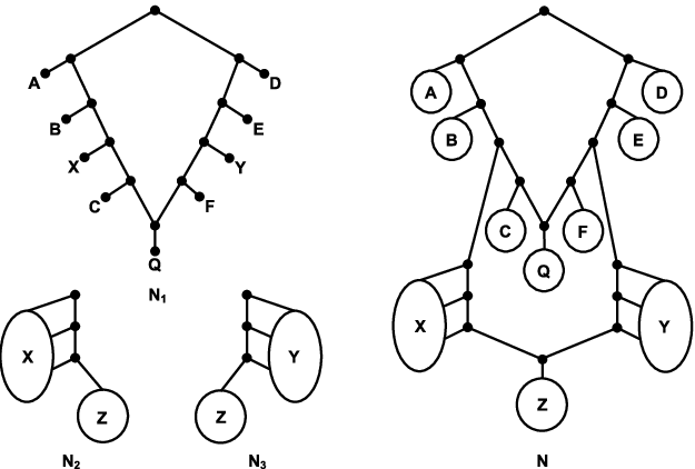

Theorem 5.1
Given a dense set of triplets , Algorithm MARLTN constructs a level-2 network that is consistent with (if such a network exists) and has a minimum number of reticulations in time.
Proof
Consider some SN-set and assume that there exists an optimal solution consistent with . The proof is by
induction on the size of . If the highest biconnected component of contains one reticulation then the
algorithm constructs an optimal solution by the proof of Theorem 3.1. Hence we assume from now on that the
highest biconnected component of contains two reticulations.
Consider the four graphs in Figure 7. Any biconnected component containing two reticulations is a
subdivision of one of these graphs [13, Lemma 13]. These graphs are called simple level-2 generators in
[13] and , , and each label, in each generator, a side of the generator, i.e. either an
arc or a vertex with indegree 2 and outdegree 0. Suppose that the highest biconnected component of is a
subdivision of generator and let the set (, , respectively) be defined as the set of leaves
reachable in from a vertex with a parent on the path corresponding to the side labelled (, ,
respectively) in .
To find an optimal network consistent with (or ) such that is below an n.c.r.-arc we
can use the following approach. If there are more than two maximal SN-sets then it is not possible. Otherwise, we
create a root and connect it to two networks for the two maximal SN-sets. If one of these maximal SN-sets contains
as a strict subset then we create a network for this set recursively. For other maximal SN-sets we use the optimal
networks computed in earlier iterations.
Given a network and a set of leaves below a cut-arc we denote by the network
obtained by removing and all vertices reachable from from , deleting all vertices with outdegree zero and
suppressing all vertices with indegree and outdegree both one.
Claim (2)
There exists an optimal solution such that the sets of leaves below highest cut-arcs of are , , and the SN-sets w.r.t. that are maximal under the restriction that they do not contain , or .
Proof
The highest biconnected component of contains just one reticulation and the same arguments can be used as in the proof of Lemma 1. ∎
Let be a network with the property described in the claim above and the collection of
sets of leaves below highest cut-arcs of . At some iteration the algorithm will consider this set
. Let equal . If we replace in each set of leaves below a highest
cut-arc by a single leaf, then we obtain a network consistent with which is either a simple
level-1 network or a path ending in a simple level-1 network, with a child of the root, the child of the
reticulation; and each vertex of the path has a leaf as child. The algorithm considers all networks of these types, so
in some iteration it will consider the right one. Let be the network constructed by the algorithm in this
iteration. It remains to prove that (i) is consistent with , (ii) contains a minimum number of
reticulations and (iii) is a level-2 network.
To prove that is consistent with , consider any triplet . First suppose that and are
all in or all in the same set of
. Then and are elements of some SN-set with
. Triplet is consistent with the subnetwork by the induction hypothesis and hence with
.
Now suppose that and are all in (or all in ). Consider the construction of the network
consistent with such that is below an n.c.r.-arc. First suppose that at some level of the recursion
there are two maximal SN-sets, each containing leaves from . Then it follows that and are in one
maximal SN-set and in the other one, by the definition of SN-set, and hence that is consistent with the
constructed network. Otherwise, and are all in some subnetwork with and is
consistent with this subnetwork (by the induction hypothesis) and hence with .
Now consider any other triplet , which thus contains leaves that are below at least two different highest
cut-arcs. Observe that the highest biconnected components of and are identical; the only differences
between these networks occur in the subnetworks below highest cut-arcs. Therefore is consistent with
since it is consistent with .
To show that contains a minimum number of reticulations consider any set of leaves below a highest cut-arc
of . The subnetwork rooted at contains a minimum number of reticulations by the induction
hypothesis. Hence contains at most as many reticulations as , which is an optimal solution.
In the networks and is the set of leaves below an n.c.r.-arc. This implies that none of the potential
reticulations in these networks end up in the highest biconnected component of . Therefore, this biconnected
component contains exactly two reticulations. All other biconnected components of also contain at most two
reticulations by the induction hypothesis. We thus conclude that is a level-2 network.
To conclude the proof we analyse the running time of the algorithm. The number of SN-sets is and hence there
are choices for each of and . For each combination of and there will be
networks constructed and for each of them it takes time to check if it is consistent with (in
line 23). Hence the overall time complexity is . ∎
6 Constructing Networks Consistent with Precisely the Input Triplet Set
In this section we consider the problem MIN-REFLECT-. Given a triplet set , this problem
asks for a level- network that is consistent with precisely those triplets in (if such a network exists)
and has minimum level over all such networks. We will show that this problem is polynomial-time solvable for each
fixed .
Recall that we use to denote the set of all triplets consistent with a network . Furthermore, we say that a
network reflects a triplet set if . The problem MIN-REFLECT- thus asks for a minimum level
network that reflects an input triplet set , for some fixed upper bound on the level of . Note that, if
reflects , that is in general not uniquely defined by . There are, for example, several distinct simple
level-2 networks that reflect the triplet set
Note that MIN-REFLECT-0 can be easily solved by using the algorithm of Aho et al. [1]. This follows because if
a tree is consistent with a dense set of triplets , then is unique [17] (and ).
Theorem 6.1. Given a dense set of triplets , it is possible to construct all
simple level- networks consistent with in time .
Lemma 4. Let be any simple network. Then all the nontrivial SN-sets of are singletons.
As we will show, the above lemma allows us to solve the problem MIN-REFLECT- by recursively constructing simple
level- networks, which we can do by Theorem 6.1. This leads to the algorithm MINPITS- (MINimum level
network consistent with Precisely the Input Triplet Set).
Theorem 6.2. Given a set of triplets , Algorithm MINPITS- solves MIN-REFLECT- in time , for any fixed
.
6.1 Constructing all simple level- networks in polynomial time
To prove Theorem 6.1 we first need several utility lemmas. Recall the concept of a simple level-k generator [13, Section 3.1]. (See also the proof of Theorem 2.)
Lemma 2
Let be a simple level- generator. Then contains vertices and arcs.
Proof
Suppose contains split vertices, reticulation vertices and 1 root. Then the total indegree equals and the total outdegree is at least . Given that the total indegree equals the total outdegree we get that and hence that . So the total number of vertices is at most . All the vertices have at most degree 3 so there are at most arcs. ∎
Lemma 3
Let be a level- network on leaves, where is fixed. Then contains vertices and arcs.
Proof
By the definition of a phylogenetic network we can view as a rooted, directed “component tree” of biconnected components where every internal vertex of represents a simple level- subnetwork of (or a single vertex), and incident arcs of an internal vertex represent arcs incident to the corresponding biconnected component. has leaves, and every internal vertex has at least two outgoing arcs. is a tree so it has at most internal vertices and thus at most vertices in total, and at most arcs. Each internal vertex represents a simple level- generator with at most arcs. Every outgoing arc raises the number of arcs (and vertices) inside the component by at most 1. So the total number of arcs in is bound above by , which is , and the total number of vertices by , also . ∎
Let be a network with at least one reticulation vertex, and let be the child of a reticulation vertex in . If has no reticulation vertex as a descendant, then we call the subnetwork rooted at a Tree hanging Below a Reticulation vertex (TBR). We additionally introduce the notion of the empty TBR, which corresponds to the situation when a reticulation vertex has no outgoing arcs. This cannot happen in a normal network but as explained shortly it will prove a useful abstraction.
Observation 1
Every network containing a reticulation vertex contains at least one TBR.
Proof
Suppose this is not true. Let be the child of a reticulation vertex in with maximum distance from the root. There must exist some vertex which is a child of a reticulation vertex and which is a descendent of . But then the distance from the root to is greater than to , contradiction.
Note that, because a TBR is (as a consequence of its definition) below a cut-arc, there exists an SN-set
w.r.t. such that is consistent with (only) the TBR. An SN-set such that is consistent with a tree,
we call a CandidateTBR SN-Set. Every TBR of corresponds to some CandidateTBR SN-Set of , but the
opposite is not necessarily true. For example, a singleton SN-set is a CandidateTBR SN-Set, but it might not be the
child of a reticulation vertex in .
We abuse definitions slightly by defining the empty CandidateTBR SN-Set, which will correspond to the empty
TBR. (This is abusive because the empty set is not an SN-set.) Furthermore we define that every triplet set has an
empty CandidateTBR SN-Set.
Observation 2
Let be a dense set of triplets on leaves. There are at most CandidateTBR SN-sets. All such sets, and the tree that each such set represents, can be found in total time .
Proof
First we construct the SN-tree for , this takes time . There is a bijection between the SN-sets of and the vertices of the SN-tree. (In the SN-tree, the children of an SN-set are the maximal SN-sets of .) Observe that a vertex of the SN-tree is a CandidateTBR SN-set if and only if it is a singleton SN-set or it has in total two children, and both are CandidateTBR SN-sets. We can thus use depth first search to construct all the CandidateTBR SN-sets; note that this is also sufficient to obtain the trees that the CandidateTBR SN-sets represent, because (for trees) the structure of the tree is identical to the nesting structure of its SN-sets. Given that there are only SN-sets, the running time is dominated by construction of the SN-tree.
Theorem 6.1
Given a dense set of triplets , it is possible to construct all simple level- networks consistent with in time .
Proof
We claim that algorithm SL- does this for us. First we prove correctness. The high-level idea is as follows.
Consider a simple level- network . From Observation 1 we know that contains at least one TBR.
(Given that is simple we know that all TBRs are equal to single leaves. That is why the outermost loop of the
algorithm can restrict itself to considering only single-leaf TBRs.) By looping through all CandidateTBR SN-sets we
will eventually find one that corresponds to a real TBR. If we remove this TBR and the reticulation vertex from which
it hangs, and then suppress any resulting vertices with both indegree and outdegree equal to 1, we obtain a new
network (not necessarily simple) with one fewer reticulation vertex than . Note that this new network might not be
a “real” network in the sense that it might have reticulation vertices with no outgoing arcs. Repeating this
times in total we eventually reach a tree which we can construct using the algorithm of Aho et al. (and is unique, as
shown in [17]). From this tree we can reconstruct the network by reintroducing the TBRs back into the
network (each TBR below a reticulation vertex) in the reverse order to which we found them. We don’t, however, know
exactly where the reticulation vertices were in , so every time we reintroduce a TBR back into the network we
exhaustively try every pair of arcs (as the arcs which will be subdivided to hang the reticulation vertex, and thus
the TBR, from.) Because we try every possible way of removing TBRs from the network , and every possible way of
adding them back, we will eventually reconstruct .
The role of the dummy leaves in SL- is linked to the empty TBRs (and their corresponding empty CandidateTBR
SN-Sets.) When a TBR is removed, it can happen (as mentioned above) that a network is created containing reticulation
vertices with no outgoing arcs. (For example: when one of the parents of a reticulation vertex from which the TBR
hangs, is also a reticulation vertex.) Conceptually we say that there is a TBR hanging below such a
reticulation vertex, but that it is empty. Hence the need in the algorithm to also consider removing the empty TBR. If
this happens, we will also encounter the phenomenon in the second phase of the algorithm, when we are re-introducing
TBRs into the network. What do we insert into the network when we reintroduce an empty TBR? We use a dummy leaf as a
place-holder, ensuring that every reticulation vertex always has an outgoing arc. The dummy leaves can be removed once
that outgoing arc is subdivided later in the algorithm, or at the end of the algorithm, whichever happens sooner. The
dummy root, finally, is needed for when there are no leaves on a side (see [13, Section 3.1]) connected to
the root.
We now analyse the running time. For we can actually generate all simple level-1 networks in time
using the algorithm in [16], and all simple level-2 networks in time using the
algorithm in [13]. For we use SL-. From Observation 2 we know that each execution of
(which computes all TBRs in a dense triplet set plus the empty TBR) takes time and
returns
at most TBRs. Operations such as computing , and the construction of the tree , all require time bounded above by
. The for loops when we “guess” the TBRs are nested to a depth of . The for loops
when we “guess” pairs of arcs from which to hang TBRs, are also nested to a depth of . (There will only
be arcs to choose from.) Checking whether
is consistent with , which we do inside the innermost loop of the entire algorithm, takes time [6, Lemma 2].
So the running time is which is . ∎
Corollary 1
For fixed and a triplet set it is possible to generate in time all simple level- networks that reflect .
Proof
The algorithm SL- (or, for that matter, the algorithms from [16][13]) can easily be adapted for this purpose: we change in line 43 “network consistent with ” to “network that reflects ”. The running time is unchanged because, whether we are checking consistency or reflection, the implementation of [6, Lemma 2] implicitly generates . ∎
6.2 From simple networks that reflect, to general networks that reflect
For a triplet and a network , we define an embedding of in as any set of four paths which, except for their endpoints, are mutually vertex disjoint, and where . We say that the vertex is the summit of the embedding. Clearly, is consistent with if and only if there is at least one embedding of in .
Lemma 4
Let be any simple network. Then all the nontrivial SN-sets of are singletons.
Proof
We prove the lemma by contradiction. Assume thus that there is some SN-set of such that .
Let be the root of . An in-out root embedding is an embedding of any triplet with and that has as its summit. We begin by proving that an in-out root embedding exists in . Suppose by contradiction this is not true. The triplet must be in because is dense and . Consider then a triplet embedding where , and . We assume without loss of generality that this embedding minimises (amongst all such embeddings) the length of the shortest directed path from to . Let be any shortest directed path from to . Now, suppose some directed path begins somewhere on the path , and intersects with the path . This is not possible because it would contradict the minimality of the length of . For the same reason, may not intersect with the path . may also not intersect with (without loss of generality) the path because this would mean . We conclude that such a path either terminates at a leaf , or re-intersects with the path . It cannot terminate at a leaf because then we either violate the minimality of the length of (because we obtain an embedding of that has a summit closer to the root than ), or we have that . We conclude that all outgoing paths from must re-intersect with . However, given that includes the root, and that in a directed acyclic graph every vertex is reachable by a directed path from the root, it follows that the last arc on the path must be a cut-arc. But this violates the biconnectivity of , contradiction. We conclude that there exists at least one in-out root embedding in .
Let be any in-out root embedding. We observe that the path must contain at least one internal vertex, by biconnectivity. Also, at least one of and must contain an internal vertex, because it is not possible for a vertex in a simple network to have two leaf children.
We now argue that there must exist a twist cover of the path . This is defined as a non-empty set of undirected paths (undirected in the sense that not all arcs need to have the same orientation) where (i) all paths in are arc-disjoint from the in-out root embedding, (ii) exactly one path starts at an internal vertex of (without loss of generality) , (iii) exactly one path ends at an internal vertex of , (iv) all other start and endpoints of the paths in lie on and (v) for every vertex of the path (including and ), there is at least one path in that has its startpoint to the left of , and its endpoint to the right. Property (v) is crucial because it says (informally) that every vertex on is “covered” by some path that begins and ends on either side of it and is arc-disjoint from the embedding. The length of is defined to be the sum of the number of arcs in each path in .
Suppose however that a twist cover does not exist. We define a partial twist cover as one that satisfies all properties of a twist cover except property (v). Partial twist covers have thus at least one vertex on that is not covered. (To see that there always exists at least one partial twist cover note that properties (ii) and (iii) in particular are satisfied by the fact that neither the removal of or can be allowed to disconnect .) So let be the partial twist cover with the maximum number of uncovered vertices. Let be the uncovered vertex that is closest to . If we removed we would, by definition, disconnect the union of the paths in with the in-out root embedding into a left part and a right part . The vertex does not, however, disconnect , so there must be some path not in that begins somewhere in and ends somewhere in . If has its startpoint on a path (where will be in ) and/or an endpoint on a path (where will be in ) then these paths can be “merged” into a new path that strictly increases the number of vertices covered. The merging occurs as follows. We take the union of the arcs in with those in and/or and discard superfluous arcs until we obtain a path that covers a strict superset of the union of the vertices covered by and/or . (In particular, the fact that begins in and ends in means that the vertex becomes covered.) In this way we obtain a new partial twist-cover with fewer uncovered vertices, contradiction. If has both its startpoint and endpoint on vertices of that are not on paths in , then can be added to the set and this extends the number of covered vertices, contradiction. If begins and/or ends elsewhere on the embedding then can be added to which again increases the number of vertices covered, contradiction. (If begins on, without loss of generality, then it becomes the new property-(ii) path and the old property-(ii) path should be discarded. Symmetrically, if ends on then it becomes the new property-(iii) path and the old property-(iii) path should be discarded.)
We conclude that for every in-out root embedding there thus exists a twist cover, and in particular a minimum length twist cover.
We observe that a minimum-length twist cover has a highly regular, interleaved structure. This regularity follows because it cannot contain paths that completely contain other paths (simply discard the inner path) and if two paths have startpoints that are both covered by some other path , and (without loss of generality) reaches further right than , then we can simply discard . For similar reasons minimum-length twist covers are vertex- and arc-disjoint. In Figure 10 we show several simple examples of twist covers exhibiting this regular structure (although it should be noted that minimum-length twist covers can contain arbitrarily many paths.)
Let be the twist cover of minimum length ranging over all in-out root embeddings of where and . Note that if contains exactly one path, which is a directed path, then (irrespective of the path orientation) , contradiction. The high-level idea is to show that we can always find, by “walking” along the paths in , a new in-out root embedding and twist cover that is shorter than , yielding a contradiction. Let be the path in that begins at , and consider the arc on this path incident to . The first subcase is if this arc is directed away from . Continuing along the path we will eventually encounter an arc with opposite orientation. This must occur before any intersection of with the path because otherwise there would be a directed cycle. Let be the vertex between these two arcs, is a reticulation vertex with indegree 2 and outdegree 1, so there must exist a directed path leaving which eventually reaches a leaf . If intersects with then we have that , contradiction. If intersects with either or then we obtain a new in-out root embedding of and a new twist cover for that embedding that is shorter than , contradiction. If does not intersect with the embedding at all, then it must be true that (because the triplet is in the network). But then we have an in-out root embedding of the triplet with twist cover shorter than , contradiction.
The second subcase (see Figure 11) is when the first arc of is entering . There must exist some directed path from to that uses this arc. The fact that is the summit of the embedding means that at some point this directed path departs from the embedding. Let be the vertex where departs from the embeddings for the last time. If is on the path then it follows that , a contradiction. If is on one of the paths or then leads to a new in-out root embedding with shorter twist cover, a contradiction. The last case is when lies on the path . We create a new in-out root embedding by using the part of reachable from , as an alternative route to . In this way becomes the “q” vertex of the new embedding (denoted in the figure). To see that we also obtain a new twist cover, note principally that paths in that covered become legitimate candidates for property-(ii) paths in the new twist cover; in the figure denotes the beginning of the property-(ii) path in the new cover. (Such a path can however partly overlap with . In this case it is necessary to first remove the part that overlaps with .) We can furthermore discard all paths from that covered except for the one with endpoint furthest to the right. Even if this means that no paths from are discarded (this happens when is to the left of all the paths in that have their beginning points on ) we still get a twist cover at least one edge smaller than , because (in particular) the first edge of is no longer needed in . In any case, contradiction. ∎


Corollary 2
Let be a set of triplets, and suppose there exists a simple network that reflects . Let be any network that reflects . Then is also simple.
Proof
If is not simple then it contains a cut-arc below which at least two leaves can be found. We know [13, Lemma 3] that every cut-arc of a network consistent with defines an SN-set w.r.t. equal to the set of leaves below it. But all the SN-sets of are singletons, contradiction. ∎
Let be a reflective set of triplets and be a network that reflects . Define as the network obtained by, for each highest cut-arc , replacing and everything below it by a single new leaf , which we identify with the set of leaves below . Let be the leaf set of . We define a new set of triplets on the leaf-set as follows: if and only if there exists and such that . We write as shorthand for the above.
Observation 3
Let be a reflective set of triplets, and let be some network that reflects . Then (1) is dense, (2) is also reflective, and reflects and (3) the maximal SN-sets of , which are in 1:1 correlation with the maximal SN-sets of , are all singletons.
Proof
The proof of (1) is trivial. For (2), observe firstly that by [13, Lemma 11.2] (the entire lemma generalises easily to higher level networks) the network is simple and consistent with . Suppose however there is some triplet that is not in . But we know then that for any the triplet is in , and thus also in , but which would mean that is in . For (3) we argue as follows. By [13, Lemma 11.3] it follows that there is a 1:1 correlation between the maximal SN-sets of and those of . Combining the fact that is reflective and that is a simple network that reflects , we can conclude from Lemma 4 that the maximal SN-sets of are all singletons. ∎
Lemma 5
Let be a reflective set of triplets and let be the maximal SN-sets of . Let be the set of triplets induced by . Let be a simple network of minimum level that reflects . Then replacing each leaf of by a network that reflects and is of minimum level amongst such networks, yields a network that reflects and is of minimum level.
Proof
We first prove that reflects . Let be any network that reflects . Every highest cut-arc of corresponds exactly to a maximal SN-set w.r.t. . Hence . Note also that for a maximal SN-set , the set of triplets is reflective: the subnetwork of below the cut-arc corresponding to reflects . (This ensures that the recursive step does find some network.) We know from Theorem 3 of [13] that the network is at least consistent with . But suppose there exists some triplet that is not in . By construction it cannot be the case that are all below the same highest cut-arc in (equivalently: in the same maximal SN-set w.r.t. ). If exactly two of the leaves are below the same highest cut-arc, then we see immediately that is in . Suppose then that all three leaves are from different maximal SN-sets , , respectively. Then because . So we can conclude the existence of some such that . But it then also follows that . We now prove that is of minimal level. Observe that all networks that reflect have the same set of highest cut-arcs, in the sense that each highest cut-arc always corresponds to exactly one maximal SN-set w.r.t. . Given that the subnetworks created for the are of minimal level, and that the level of is equal to the maximum level ranging over and all subnetworks below highest cut-arcs, it follows that is of minimum level if and only if is of minimum level. ∎
Theorem 6.2
For fixed we can solve MIN-REFLECT- in time
Proof
From Observation 3 we know that there is no solution if is not dense, and this can be checked in time. We henceforth assume that is dense. For we can simply use the algorithm of Aho et al., which (with an advanced implementation [17]) can be implemented to run in time , which is . For we use algorithm MINPITS-. Correctness of the algorithm follows from Lemma 5. It remains to analyze the running time. A simple level- network (that reflects the input) can be found (if it exists) in time using algorithm SL-. (To find the simple network of minimum level we execute in order SL-1, SL-2, …, SL- until we find such a network. This adds a multiplicative factor of to the running time but this is absorbed by the notation for fixed .) Therefore, lines 6 and 7 of MINPITS- take time. At every level of the recursion the computation of the maximal SN-sets of can be done in time , and computation of also takes . The critical observation is that (by Observation 3) every SN-set in appears exactly once as a leaf inside an execution of SL-. The overall running time is thus of the form where is equal to the total number of SN-sets in . Noting that , and that there are at most SN-sets in , we obtain for an overall running time of , which is because is dense. ∎
7 Conclusions and open questions
In this article we have shown that, for level 1 and 2, constructing a phylogenetic network consistent with a dense set
of triplets that minimises the number of reticulations (i.e. DMRL-1 and DMRL-2), is polynomial-time solvable. We feel
that, given the widespread use of the principle of parsimony within phylogenetics, this is an important development,
and testing on simulated data has yielded promising results. However, the complexity of finding a feasible
solution for level-3 and higher, let alone a minimum solution, remains unknown, and this obviously requires attention.
Perhaps the feasibility and minimisation variants diverge in complexity, for high enough , it would be fascinating
to explore this.
We have also shown, for every fixed , how to generate in polynomial time all simple level- networks consistent with
a dense set of triplets. This could be an important step towards determining whether the aforementioned feasibility question
is tractable for every fixed . We have used the SL- algorithm to show how, for every fixed , MIN-REFLECT- is
polynomial-time solvable. Clearly the demand that a set of triplets is exactly equal to the set of triplets in some network
is an extremely strong restriction on the input. However, for small networks and high accuracy triplets
such an assumption might indeed be valid, and thus of practical use. In any case, the concept of reflection is likely
to have a role in future work on “support” for edges in phylogenetic networks generated via triplets. Also, there remain some
fundamental questions to be answered about reflection. For example, the complexity of the question “does any network
reflect ?” remains unclear.
Acknowledgements
We thank Judith Keijsper, Matthias Mnich and Leen Stougie for many helpful discussions during the writing of the paper.
References
- [1] A.V. Aho, Y. Sagiv, T.G. Szymanski and J.D. Ullman, Inferring a Tree from Lowest Common Ancestors with an Application to the Optimization of Relational Expressions, SIAM Journal on Computing, 10 (3), pp. 405-421 (1981).
- [2] M. Baroni, S. Grünewald, V. Moulton and C. Semple, Bounding the Number of Hybridisation Events for a Consistent Evolutionary History, Mathematical Biology, 51, pp. 171-182 (2005).
- [3] M. Baroni, C. Semple, M. Steel, A Framework for Representing Reticulate Evolution, Annals of Combinatorics, 8, pp. 391-408 (2004).
- [4] M. Bordewich, C. Semple, Computing the Minimum Number of Hybridization Events for a Consistent Evolutionary History, Discrete Applied Mathematics, 155 (8), pp. 914-928 (2007).
- [5] M. Bordewich, S. Linz, K. St. John, C. Semple, A Reduction Algorithm for Computing the Hybridization Number of Two Trees, Evolutionary Bioinformatics, 3, pp. 86-98 (2007).
- [6] J. Byrka, P. Gawrychowski, S.M. Kelk and K.T. Huber, Worst-case optimal approximation algorithms for maximizing triplet consistency within phylogenetic networks, arXiv:0710.3258v3 [q-bio.PE] (2008).
- [7] C. Choy, J. Jansson, K. Sadakane and W.-K. Sung, Computing the Maximum Agreement of Phylogenetic Networks, Theoretical Computer Science, 335 (1), pp. 93-107 (2005).
- [8] S. Guindon and O. Gascuel, A Simple, Fast, and Accurate Algorithm to Estimate Large Phylogenies by Maximum Likelihood, Systematic Biology, 52 (5), pp. 696-704 (2003).
- [9] D. Gusfield, S. Eddhu and C. Langley, Optimal, Efficient Reconstructing of Phylogenetic Networks with Constrained Recombination, Journal of Bioinformatics and Computational Biology, 2 (1), pp. 173-213 (2004).
- [10] D. Gusfield, D. Hickerson and S. Eddhu, An Efficiently Computed Lower Bound on the Number of Recombinations in Phylognetic Networks: Theory and Empirical Study, Discrete Applied Mathematics, 155 (6-7), pp. 806-830 (2007).
- [11] J. Hein, Reconstructing Evolution of Sequences Subject to Recombination Using Parsimony, Mathematical Biosciences, 98, pp. 185-200 (1990).
- [12] D.H. Huson and D. Bryant, Application of Phylogenetic Networks in Evolutionary Studies, Molecular Biology and Evolution, 23 (2), pp. 254-267 (2006).
- [13] L.J.J. van Iersel, J.C.M. Keijsper, S.M. Kelk and L. Stougie, Constructing Level-2 Phylogenetic Networks from Triplets, arXiv:0707.2890v1 [p-bio.PE] (2007).
- [14] L.J.J. van Iersel, J.C.M. Keijsper, S.M. Kelk, L. Stougie, F. Hagen and T. Boekhout, Constructing Level-2 Phylogenetic Networks from Triplets, in Proceedings of Research in Computational Molecular Biology (RECOMB 2008), LNBI 4955, pp. 464-476 (2008).
- [15] L.J.J. van Iersel, S.M. Kelk and M. Mnich, Uniqueness, Intractability and Exact Algorithms: Reflections on Level-k Phylogenetic Networks, arXiv:0712.2932v2 [q-bio.PE] (2007).
- [16] J. Jansson, N.B. Nguyen and W.-K. Sung, Algorithms for Combining Rooted Triplets into a Galled Phylogenetic Network, SIAM Journal on Computing, 35 (5), pp. 1098-1121 (2006).
- [17] J. Jansson and W.-K. Sung, Inferring a Level-1 Phylogenetic Network from a Dense Set of Rooted Triplets, Theoretical Computer Science, 363, pp. 60-68 (2006).
- [18] V. Makarenkov, D. Kevorkov and P. Legendre, Phylogenetic Network Reconstruction Approaches, in Applied Mycology and Biotechnology, International Elsevier Series 6, Bioinformatics, pp. 61-97 (2006).
- [19]
MARLON: Constructing Level One Phylogenetic Networks with a Minimum Amount of Reticulation,
http://homepages.cwi.nl/
~kelk/marlon.html. - [20] D.A. Morrison, Networks in Phylogenetic Analysis: New Tools for Population Biology, International Journal for Parasitology, 35 (5), pp. 567-582 (2005).
- [21] B.M.E. Moret, L. Nakhleh, T. Warnow, C.R. Linder, A. Tholse, A. Padolina, J. Sun, and R. Timme, Phylogenetic Networks: Modeling, Reconstructibility, and Accuracy, IEEE/ACM Transactions on Computational Biology and Bioinformatics, 1 (1), pp. 13-23 (2004).
- [22] A. Rambaut and N.C. Grassly, Seq-Gen: An Application for the Monte Carlo Simulation of DNA Sequence Evolution along Phylogenetic Trees, Computer Applications in the Biosciences, 13, pp. 235-238 (1997).
- [23] Y.S. Song, J. Hein, On the Minimum Number of Recombination Events in the Evolutionary History of DNA Sequences, Journal of Mathematical Biology, 48, pp. 160186 (2004).
- [24] Y.S. Song, Y. Wu, D. Gusfield, Efficient Computation of Close Lower and Upper Bounds on the Minimum Number of Recombinations in Biological Sequence Evolution, Bioinformatics, 21 (Suppl. 1), pp. i413 - i422 (2005).
- [25] L. Wang, K. Zhang, L. Zhang, Perfect Phylogenetic Networks with Recombination, Journal of Computational Biology, 8 (1), pp. 69-78 (2001).