Coherent state quantization of angle, time, and more irregular functions and distributions
Abstract
The domain of application of quantization methods is traditionally restricted to smooth classical observables. We show that the coherent states or “anti-Wick” quantization enables us to construct fairly reasonable quantum versions of irregular observables living on the classical phase space, such as the angle function, the time function of a free particle and even a large set of distributions comprising the tempered distributions.
1 Introduction
In this work, we reexamine the way in which Gaussian (or standard) coherent states (CS) allow a natural quantization (“Berezin-Klauder CS or anti-Wick quantization”) of the complex plane viewed as the phase space of the particle motion on the line. First, we extend the definition of what should be considered as an acceptable quantum observable. Then, we prove that many classical singular functions give rise to such reasonable quantum operators. More precisely, we apply the CS quantization scheme to classical observables which are not smooth functions or, even more, which are, with mild restrictions, distributions on the plane. In particular, this departure from the canonical quantization principles allows us to put in a CS diagonal form the argument function and the time function of a free particle . We also consider the Dirac distribution on the plane and its derivatives, and this allows us to reach any kind of finite-dimensional projector on the Hilbert space of quantum states. Finally, we extend this quantization scheme to a set of distributions which includes the space of tempered distributions.
The motivation for enlarging the space of quantizable classical observable also stems from the fact that this coherent state quantization can have possible applications in a wide variety of physical problems, like the long standing and controversial question of the determination and the study of the time operator for an interacting particle (see [1] and references therein). This aspect will be considered in this paper in the simplest case of the one-dimensional motion of a free particle (the quantization of ) or of the harmonic oscillator (angle operator). Our approach has also possible implications in noncommutative (NC) quantum mechanics, which is being currently studied for its possible application in fractional Quantum Hall Effect (FQHE): If one considers the Landau problem in a 2D plane, the commutators of the projected and coordinate operators of a particle onto the lowest Landau level give rise to noncommutativity in terms of the inverse of the applied magnetic field [2]. One is therefore led to study the planar NC quantum mechanics per se, where the “classical” Hilbert space itself corresponds to the Hilbert space of quantum states for the particle motion on the line. The quantum Hilbert space for this planar NC system is thus identified with the set of all bounded operators in this classical Hilbert space, with respect to a certain inner product [3]. One can then introduce a disk [3] or defects [4] in the NC plane in terms of these projectors in the classical Hilbert space. These defects, on turn, can give rise to certain edge states, relevant for FQHE.
2 The Berezin-Klauder or anti-Wick quantization of the motion of a particle on the line
Let us consider the quantum motion of a particle on the real line. On the classical level, the phase space (with suitable physical units) reads as . This phase space is equipped with the ordinary Lebesgue measure on the plane which coincides with the symplectic 2-form : where . Strictly included in the Hilbert space of all complex-valued functions on the complex plane which are square-integrable with respect to this measure, there is the Fock-Bargmann Hilbert subspace of all square integrable functions which are of the form where is analytical entire. As an orthonormal basis of this subspace we have chosen the normalized powers of the conjugate of the complex variable weighted by the Gaussian function, i.e. with . Normalized coherent states are well known [5, 6, 7, 8] and read as the following superposition of number eigenstates:
| (1) |
We here recall one fundamental feature of the states (1), namely the resolution of the unity in the Hilbert space having as orthonormal basis the set of :
| (2) |
The property (2) is crucial for our purpose in setting the bridge between the classical and the quantum world. It encodes the quality of coherent states of being canonical quantizers [9] along a guideline established by Klauder and Berezin (and also Toeplitz on a more abstract mathematical level). This Berezin-Klauder-Toeplitz (BKT) (or anti-Wick, or anti-normal) coherent states quantization, called hereafter CS quantization, consists in associating with any classical observable , that is a (usually supposed smooth, but we will not retain here this too restrictive attribute) function of phase space variables or equivalently of , the operator-valued integral
| (3) |
The resulting operator , if it exists, at least in a weak sense, acts on the Hilbert space . It is worthy to be more explicit about what we mean by “weak sense”: the integral
| (4) |
should be finite for any (or some dense subset in ). One notices that if is normalized then (4) represents the mean value of the function with respect to the -dependent probability distribution on the phase space.
More mathematical rigor is necessary here, and we will adopt the following acceptance criteria for a function (or distribution) to belong to the class of quantizable classical observables.
Definition 2.1.
A function and more generally a distribution is a CS quantizable classical observable along the map defined by (3), and more generally by ,
- •
if the map (resp. ) is a smooth () function with respect to the coordinates of the phase plane.
- •
and, if we restore the dependence on through , we must get the right semi-classical limit, which means that . The same asymptotic behavior must hold in a distributional sense if we are quantizing distributions.
The function (resp. the distribution ) is an upper or contravariant symbol of the operator (resp. ), and the mean value (resp. ) is the lower or covariant symbol of the operator (resp. ). The map is linear and associates with the function the identity operator in . Note that the lower symbol of the operator is the Gaussian convolution of the function :
| (5) |
This expression is of great importance and is actually the reason behind the robustness of CS quantization, since it is well defined for a very large class of non smooth functions and even for a class of distributions comprising the tempered ones. Equation (5) illustrates nicely the regularizing role of quantum mechanics versus classical singularities. Note also that the Gaussian convolution helps to carry out the semi-classical limit, since the latter can be extracted by using a saddle point approximation. For regular functions for which exists, the application of the saddle point approximation is trivial and we have
| (6) |
For singular functions the semi-classical limit is less obvious and has to be verified for each special case, something we will do systematically for those ones considered in the following sections. Also, this particular aspect of CS quantization can be very useful in the context of the quantum mechanical problem of particles moving in the NC plane, as we had mentioned earlier [3]. Since in this context the quantum Hilbert space comprises the bounded operators in the classical Hilbert space, one can recover the usual coordinate space wave function by taking expectation values of these operators in the coherent state family (1), i.e. by obtaining the corresponding lower symbol [10].
Now let us make the CS quantization program more explicit. Expanding bras and kets in (3) in terms of the Fock states yields the expression of the operator in terms of its infinite matrix elements :
| (7) |
In the case where the classical observable is “isotropic”, i.e. , then is diagonal, with matrix elements given by a kind of gamma transform:
| (8) |
In the case where the classical observable is purely angular-dependent, i.e. for , the matrix elements are obtained through a Fourier transform:
| (9) |
where is the Fourier coefficient of the -periodic function . Thus we have in this case:
| (10) |
Let us explore what this quantization map produces starting with some elementary functions . We have for the most basic one,
| (11) |
which is the lowering operator, . The adjoint is obtained by replacing by in (11). From et , one easily infers by linearity that the canonical position and momentum map to the quantum observables and respectively. In consequence, the self-adjoint operators and obtained in this way obey the canonical commutation rule , and for this reason fully deserve the name of position and momentum operators of the usual (galilean) quantum mechanics, together with all localization properties specific to the latter.
3 Canonical quantization rules
At this point, it is worthy to recall what quantization of classical mechanics does mean in a commonly accepted sense (for a recent review see [11]). In this context, a classical observable is supposed to be a smooth function with respect to the canonical variables. In the above we have chosen units such that the Planck constant is just put equal to 1. Here we reintroduce it since it parametrizes the link between classical and quantum mechanics.
Van Hove canonical quantization rules [12]
Given a phase space with canonical coordinates
- (i)
to the classical observable corresponds the identity operator in the (projective) Hilbert space of quantum states,
- (ii)
the correspondence that assigns to a classical observable , a self-adjoint operator on is a linear map,
- (iii)
to the classical Poisson bracket corresponds, at least at the order , the quantum commutator, multiplied by :
- (iv)
some conditions of minimality on the resulting observable algebra.
The last point can give rise to technical and interpretational difficulties [11].
It is clear that points (i) and (ii) are fulfilled with the CS quantization, the second one at least for observables obeying fairly mild conditions. In order to better understand the “asymptotic” meaning of Condition (iii), let us quantize higher degree monomials, starting with , the classical harmonic oscillator Hamiltonian. For the latter, we get immediately from (8):
| (12) |
where is the number operator. We see on this elementary example that the CS quantization does not fit exactly with the canonical one, which consists in just replacing by and by in the expressions of the observables and next proceeding to a symmetrization in order to comply with self-adjointness. In fact, the quantum Hamiltonian obtained by this usual canonical procedure is equal to . In the present case, there is a shift by between the spectrum of and our coherent state quantized Hamiltonian . Actually, it seems that no physical experiment can discriminate between those two spectra that differ from each other by a simple shift (for a deepened discussion on this point, see for instance [13]), unless one couples the system with gravity which couples to any system carrying energy and momentum. 11 1 This can be considered, on a quite elementary level, as a facet of the cosmological constant problem, since the inclusion of a cosmological constant corresponds to a shift in the Hamiltonian . See [14] for a review on this question. In the same spirit, Wigner showed in [15] that the usual canonical commutation relation is not the only one compatible with the requirement that the quantum operators in the Heisenberg picture obey the classical equations of motion. In fact for the harmonic oscillator (with unit mass and frequency) a whole family of commutation relations parametrized by the ground state energy are admissible: (13) The canonical commutation relations correspond to . The CS quantization gives which would correspond to in the Wigner quantization scheme, and so should entail a (non-canonical!) redefinition of position and momentum, something like . At this stage, let us recall that the vacuum energy of a free scalar field of mass is given by and it is worth noting that the quantization ambiguity showed by Wigner does not allow , with all the implications to the cosmological constant problem that such a semi-classical computation would have.
Let us add for future references the quantization of the Hamiltonian of a free particle moving on the line. The Hamiltonian for the free particle of unit mass is . With the Hamiltonian is . Using the expression (7) we get the quantum Hamiltonian operator
| (14) |
We also observe that the lower symbol is exactly equal to the classical Hamiltonian for any value of
| (15) |
4 More upper and lower symbols: the angle operator
Since we do not retain in our quantization scheme the condition of smoothness on the classical observables, we feel free to CS quantize a larger class of functions on the plane, like the argument of the complex variable . The function is infinite-valued with a branch cut starting from the origin which is a branching point. Computing its quantum counterpart from (9) is straightforward and yields the infinite matrix:
| (16) |
The corresponding lower symbol reads as the Fourier sine series:
| (17) |
where
| (18) | |||||
We can also write an integral representation of the lower symbol using the convolution (5)
Let us verify that this lower symbol is as a function of and in conformation with our definition 2.1. First we note that
where and are polynomials in the variables and are positive integers. Then we use the asymptotic formula for large order of the Bessel function [16]
| (19) |
This makes the series and absolutely convergent, and thus is for . The behavior of the lower symbol (17) is shown in Figure 1.


It is interesting to evaluate the asymptotic behaviors of the function (17) at small and large respectively. At small , it oscillates around its average value with amplitude equal to :
At large , we recover the Fourier series of the -periodic angle function:
The latter result can be equally understood in terms of classical limit of these quantum objects. Indeed, by re-injecting into our formula physical dimensions, we know that the quantity acquires the dimension of an action and should appear in the formulas as divided by the Planck constant . Hence, the limit in our previous expressions can also be considered as the classical limit . Since we have at our disposal the number operator , which is up to a constant shift the quantization of the classical action, and an angle operator, we can examine their commutator and its lower symbol in order to see to what extent we get something close to the expected canonical value, namely . The commutator reads as
| (20) |
Its lower symbol is then given by
| (21) |
with the same as in (17).
At small , the function oscillates around with amplitude equal to :
At large , the function tends to the Fourier series whose convergence has to be understood in the sense of distributions. Applying the Poisson summation formula, we get at (or ) the expected “canonical” behavior for . The fact that this commutator is not exactly canonical was expected since we know from Dirac [17] about the impossibility to get canonical commutation rules for the quantum versions of the classical canonical pair action-angle. On a more general level, we know that there exist such classical pairs for which mathematics -e.g. the Pauli theorem-[18] prevent the corresponding quantum commutator of being exactly canonical. We will discuss this point in more details when quantizing the time function in the next section. However, in the present case, we obtain in the quasi-classical regime the following asymptotic behavior:
| (22) |
One can observe that the commutator symbol becomes “canonical” for . Dirac singularities are located at the discontinuity points of the periodic extension of the linear function for .
5 Classical and quantum time of the free particle
The quantization of the time function is, like for the angle, an old, important, and controversial question [1]. Aside from conceptual problems, the basic difficulty encountered in the construction of a quantum time operator is summarized in the called Pauli theorem [18, 19, 20, 21]: one would expect naively the time operator to be conjugated to the Hamiltonian . However if one assumes that is a bounded from below operator, such a commutation relation cannot hold. The Hamiltonian for the free particle, , implies (up to the addition of a constant). We can invert this relation to get an expression of the classical time as a function on the phase space . If we view the phase space as the complex plane by setting , then the classical time function is . Since the time function is only dependent , its CS quantized version is given by (10) . The coefficients are given by
| (23) |
The first integral is singular and we will understand it as a principal value, for instance, . For parity reasons the real part of is zero and
The time operator is thus given by:
| (24) |
and the lower symbol is:
| (25) |
where
| (26) | |||||
One can also prove that this lower symbol is exactly in the same way we proved that is . It is also important to control the semi-classical limit, which appears as
| (27) |

5.1 The commutator
Using the expressions of the time and Hamiltonian operators, we can compute the commutator :
| (28) |
The question now is to evaluate the extent to which this commutator is different from the canonical . First we notice that this matrix shares the same diagonal part as the canonical commutator and is well localized along its diagonal since asymptotically the coefficients are rapidly decreasing away from the diagonal. For instance, for large , we have , which goes to more rapidly than . Figure 3 shows this localization.
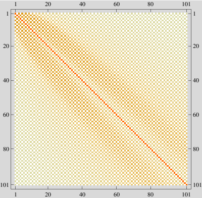
In order to go further in the comparison of our commutator with the canonical one, we numerically study its spectrum by truncating the infinite matrix. The results are shown in figure 4 and confirms that the spectrum of the commutator is very close to that of the canonical spectrum with infinite degeneracy.

To study further the departure from the canonical value of the commutator, let us define the operator . First we note that is a trace class operator, since . We note also that is not a Hilbert-Schmidt operator because
is a divergent sum. We have carried out a numerical analysis to find the spectrum of the operator and we find that this spectrum is bounded and seems to verify . Thus the spectral norm of , given by is well defined. Numerically its value is equal to 1 as shown in Figure 5.

The lower symbol of the commutator can be written as the following sum
| (29) |
where
| (30) |
Restoring the units, we can verify that this commutator has the canonical form in the semi-classical limit , since in this limit we have .
6 Quantization of distributions: Dirac and others
It is commonly accepted that a “CS diagonal” representation of the type (3) is possible only for a restricted class of operators in . The reason is that we usually put too much restrictive conditions on the upper symbol viewed as a classical observable on the phase space, and so it is submitted to belong to the space of infinitely differentiable functions on . We already noticed that a “reasonable” phase or angle operator is easily built starting from the classical discontinuous periodic angle function. We are now going to show that any simple projector has also a CS diagonal representation by extending the class of classical observables to distributions on (for canonical coordinates or possibly on (for coordinates). Due to the general expression (7) for matrix elements of the quantized version of an observable , one can immediately think to tempered distributions on the plane only since the functions
| (31) |
are rapidly decreasing functions on the plane with respect to the canonical coordinates , i.e. they belong to the Schwartz space , or equivalently with respect to the coordinates . Actually, we can extend the set of “acceptable” observables to those distributions in which obey the following condition (similar extensions to distributions have been considered in [8], and [22, 23] for the Weyl quantization).
Proposition 6.1.
A distribution is a CS quantizable classical observable if there exists such that the product , i.e. is a tempered distribution.
Using complex coordinates is clearly more convenient and we will adopt the following definitions and notations for tempered distributions. Firstly any function which is “slowly increasing” and locally integrable with respect to the Lebesgue measure on the plane defines a regular tempered distribution , i.e. a continuous linear form on the vector space equipped with the usual topology of uniform convergence at each order of partial derivatives multiplied by polynomial of arbitrary degree [24]. This definition rests on the map,
| (32) |
and the notation is kept for all tempered distributions . According to Proposition 6.1, this definition can be extended to locally integrable functions which increase like for some and some polynomial , and it is easily understood in which way this extends to distributions. Actually, the latter can be characterized as derivatives (in the distributional sense) of such functions. We recall here that partial derivatives of distributions are given by
| (33) |
We also recall that the multiplication of distributions by smooth functions is understood through:
| (34) |
Of course, all compactly supported distributions like Dirac and its derivatives, are tempered and so are CS quantizable classical observable. The Dirac distribution supported by the origin of the complex plane is denoted as usual by (and abusively in the present context by ) :
| (35) |
| (36) |
We thus find that the ground state (as a projector) is the quantized version of the Dirac distribution supported by the origin of the phase space. The obtention of all possible diagonal projectors or even all possible oblique projectors is based on the quantization of partial derivatives of the distribution. First let us compute the various derivatives of the Dirac distribution:
| (37) |
Once this quantity at hand, one can invert the formula in order to get the oblique projector as:
| (38) |
and its upper symbol are given by the distribution supported by the origin:
| (39) |
Note that this distribution, as is well known, can be approached, in the sense of the topology on , by smooth functions, like linear combinations of derivatives of Gaussians. The diagonal projectors are then obtained trivially by setting in (38) to get
| (40) |
Again in the context of quantum mechanics in the NC plane, one notes that one can define a projection operators to define an analogue of a disk [3]. On the other hand, the removal of the “disk” from the classical Hilbert space defines an analogue of a defect in the NC plane [4].
Using the expressions of the projectors and the linearity of the quantization map , one can formally construct an inversion (dequantization) operator given by:
| (41) |
This inversion map also enables us to construct a star product on the classical phase space verifying (See for instance [25] for a general review on deformation quantization,and [26, 27, 28, 29] for more material based on coherent states)
Note that this star product involves the upper symbols, in contrast to the Voros star product [26, 27, 28, 29], which involves the lower symbols.
Many of the ideas around this combination of coherent states with distributions pertain to the domain of Quantum Optics. They are already present in the original works by Sudarshan [8], Glauber [33], Klauder [30], Cahill [31], Miller [32] and others. In Quantum Optics the basic idea is that replacing the non diagonal representation of quantum operators (usually, in this context, one focuses on the density operators ) given by
by a diagonal one, also called the -representation, , can simplify considerably some calculations. Although this can be considered as the CS quantization of , the spirit is quite different since their approach is the inverse of ours: given , then the question is to find . The main results obtained in this direction is that one can formally write a -representation for each quantum operator , which is given by [8]
| (42) |
or by [30]
| (43) |
Here is the Fourier transform from the -space to the -space, and is its inverse. However the question of the validity of such formulas is mathematically non trivial: the convergence in the sense of distributions of (41,42) is a difficult problem, and for instance has been partially studied by Miller in [32] Manifestly, the work done in this direction was concentrated on the dequantization problem (finding an associated classical function to each quantum operator) and this was done in a quite pragmatic spirit in order to simplify computations. Let us note that the existence of such a well-defined dequantization procedure is by no means a physical requirement since the quantum realm is by definition richer than the classical one. A more physical requirement is that the semi-classical limit is well behaved, a property that we have placed at the center of our work.
7 Application of coherent state formulation in a planar NC system
As was introduced in [3] the classical Hilbert space for a planar noncommutative system satisfying is identified as the boson Fock space
| (44) |
constructed out of the bosonic creation and annihilation operators and respectively satisfying . On the other hand the quantum Hilbert space is identified as the set of bounded operators on :
| (45) |
Here the inner product between any pair of states and is defined as a trace in the classical Hilbert space
| (46) |
Note that we are denoting the vectors belonging to and by and respectively. Thus the coherent state introduced in (1), which provides an overcomplete system for the quantum Hilbert space of states for a particle moving in a line, now corresponds to the over-complete basis for the classical Hilbert space (44) as well, as these two Hilbert spaces are really isomorphic to each other. Consequently, the inner product can be calculated by using either the countable basis or coherent state family
| (47) |
Using this one can identify the normalized momentum eigenstate as
| (48) |
which are nothing but the operator-valued plane-wave states-a direct generalization from the commutative case. The fact that these plane waves are really the momentum eigenstates can be checked easily by considering the adjoint action of momentum on the state [2]
| (49) |
to get
| (50) |
The adjoint action of the momentum (49) along with left action of the coordinate operator on the elements of the quantum Hilbert space
| (51) |
describes the complete action of the phase space operators on satisfying the noncommutative Heisenberg algebra [2]. Now using the fact that we can introduce as an upgraded version of the overcomplete coherent states in satisfying
| (52) |
Following [10], we can now construct the ‘position’ representation of a state as
| (53) |
which clearly corresponds to a lower symbol of the operator . In particular the position representation of the momentum eigenstates (48) turns out to be
| (54) |
Using this one can easily show that
| (55) |
implying that really forms a total family solving the identity in
| (56) |
On the other hand
| (57) |
showing that the naive resolution of identity, the counterpart of (2) in , fails in this case
| (58) |
However, as we have mentioned in the preceding section, that lower symbols should be composed through the Voros star product ([26, 29]) as
| (59) |
Once done that, we can readily verify that
| (60) |
so that the appropriate resolution of identity in is given by
| (61) |
Finally note that any element can be expanded in terms of the oblique operators as,
| (62) |
implying that the oblique projectors provide a complete set of states in . Alternatively it follows from (38) that states also provide an overcomplete set if the coefficient involve the derivatives of Dirac’s distribution function in “position space” which should also compose through Voros star product.
Extension of this analysis involving the formulation of NC Quantum Mechanics in 3D is rather non-trivial as the rotational invariance is broken in presence of such a constant(non-transforming) antisymmetric matrix satisfying as the dual vector is pointed to a particular direction in space and which can only be restored by a twisted implementation of the rotation group (SO(3)) in a Hopf algebraic setting [35]. However one has to sacrifice the vectorial transformation property of the coordinate operators in D3, which can now be identified as the primitive linear operators in a deformed Hopf algebra [36]. Further work in this direction is in progress and will be reported later.
8 Concluding remarks
In this paper, we have established that the CS quantization map enables us to quantize singular classical functions, and, more generally, distributions including tempered distributions. More precisely, we are able to construct a reasonable and well behaved quantum angle and time operator for the free particle moving on the line. In particular our time operator is hermitian, verifies the canonical commutation relation with the Hamiltonian up to order , and has the right semi-classical limit. Let us point out the relevance of our work to the study of a “phase space formulation” of quantum mechanics, which enables to mimic at the level of functions and distributions the algebraic manipulations on operators within the quantum context. In particular, by carrying out the CS quantization of Cartesian powers of planes, we could so have at our disposal an interesting “functional portrait” in terms of a “star” product on distributions for the quantum logic based on manipulations of tensor products of quantum states.
Acknowledgment
One of us, BC would like to thank F. G. Scholtz and S. Vaidya for discussion.
References
- [1] Y. Aharonov and D. Bohm, Phys. Rev. 122 1649-1658 (1961); D. H. Kobe and V. C. Aguilera-Navarro Derivation of the energy-time uncertainty relation, Phys. Rev. A 50, 933-937 (1994); P. Pfeifer and J. Frohlich, Rev. Mod. Phys. 67, 759 (1995); P. Busch The Time-Energy Uncertainty Relation, arXiv:quant-ph/0105049 v2 10 Oct 2004.
- [2] R. Szabo, Quantum Field Theory on Noncommutative space, Phys. Rep. 378, 207-299 (2003)
- [3] F. G. Scholtz, B. Chakraborty, J. Govaerts and S. Vaidya, Spectrum of the noncommutative spherical well, J. Phys. A 40 14581-14592 (2007)
- [4] A. Pinzul and A. Stern, Edge states from defects on the noncommutative plane, Mod. Phys. Lett. A 18, 2509-2516 (2003)
- [5] E. Schrödinger, Der stetige Übergang von der Mikro- zur Makromechanik, Naturwiss. 14, 664-666 (1926).
- [6] J. R. Klauder, The Action Option and the Feynman Quantization of Spinor Fields in Terms of Ordinary c-Numbers, Annals of Physics 11, 123-168 (1960); J. R. Klauder, Continuous-Representation Theory I. Postulates of continuous-representation theory, J. Math. Phys. 4, 1055-1058 (1963).
- [7] R. J. Glauber, Photons correlations, Phys. Rev. Lett. 10, 84-86 (1963).
- [8] E. C. G. Sudarshan, Equivalence of Semiclassical and Quantum Mechanical Descriptions of Statistical Light Beams, Phys. Rev. Letters 10, 277 (1963).
- [9] F. A. Berezin, General concept of quantization, Commun. Math. Phys. 40, 153-174 (1975).
- [10] J. M. Gracia-Bondia and J. C. Varilly, Algebra of distributions suitable for phase space quantum mechanics, J. Math. Phys. 29, 869 (1998).
- [11] S. T. Ali and M. Englis, Quantization methods: a guide for physicists and analysts, math-ph/0405065v1 (2004).
- [12] L. Van Hove, Sur le problme des relations entre les transformations unitaires de la Mcanique quantique et les transformations canoniques de la Mcanique classique, Bull. Acad. Roy. Belg., cl. des Sci. 37, 610-620 (1961).
- [13] H. A. Kastrup, A new look at the quantum mechanics of the harmonic oscillator, Ann. Phys. (Leipzig) 7-8, 439-528 (2007).
- [14] S. Weinberg, The cosmological constant problem, Rev. Mod. Phys. 61, 1-23 (1989).
- [15] E. P. Wigner, Do the equations of motion determine the quantum mechanical commutation relations?, Phys. Rev. 77, 711 (1950).
- [16] G. N. Watson, A treatise on the theory of Bessel functions, Cambridge Mathematical Library (1995).
- [17] P. A. M. Dirac Proc. R. Soc. London Ser. A 114, 243-265 (1927).
- [18] W. Pauli, Die allgemeinen Prinzipien der Wellenmechanik, Hanbuck der Physik, vol. 1, Springer Verlag, Berlin (1958).
- [19] E. Galapon, Proc. R. Soc. Lond. A 458, 451-472 (2002).
- [20] R. Giannitrapani, [arXiv: quant-ph/0302056] (2002).
- [21] M. Toller, gr-qc/9605052 v1 (1996).
- [22] P. Boggiatto, E. Cordero Anti-Wick quantization of tempered distributions, Progress in analysis, Vol. I, II, Berlin (2001), 655-662, World Sci. Publ., River Edge, NJ (2003).
- [23] P. Boggiatto, E. Cordero, K. Grchenig Generalized Anti-Wick Operators with Symbols in Distributional Sobolev spaces, Integral Equations Operator Theory 48, no. 4, 427-442 (2004).
- [24] L. Schwartz, Mthodes mathmatiques pour les sciences physiques, Hermann (1961).
- [25] A. C. Hirshfeld, P. Henselder, Deformation Quantization in the Teaching of Quantum Mechanics, quant-ph/0208163 (2002).
- [26] A. Voros, Wentzel-Kramers-Brillouin method in the Bargman representation, Phys. Rev. A 40, 6814-6825 (2002).
- [27] M. Daoud, Extended Voros product in the coherent states framework, Phys. Lett. A 309, 167-175 (2003).
- [28] G. Alexanian, A. Pinzul, A. Stern, Generalized coherent state approach to star products and applications to the fuzzy sphere, Nuc. Phys. B 600, 531-547 (2001).
- [29] A.P.Balachandran, S.Kurkcuoglu and S.Vaidya, Lectures on Fuzzy and Fuzzy SUSY Physics, World Scientific, Singapore (2007).
- [30] J. R. Klauder, Fundamentals of Quantum Optics, (1968).
- [31] K. E. Cahill, Coherent-State Representations for the Photon Density, Phys. Rev. 138, B1566 (1965).
- [32] M. M. Miller, Convergence of the Sudarshan Expansion for the Diagonal Coherent-State Weight Functional, J. Math. Phys. 9, 1270 (1968).
- [33] R. J. Glauber, The quantum theory of optical coherence, Phys. Rev. 130, 2529 (1963).
- [34] R. J. Glauber, Coherent and incoherent states of radiation field, Phys. Rev. 131, 2766 (1963).
- [35] See for example the recent review: E. Akofor, A. P. Balachandran, A. Joseph,Quantum Fields on the Groenewold-Moyal Plane, Int. J. Mod. Phys. A23:1637-1677 (2008) and the references therein.
- [36] P.G Castro, B. Chakraborty, and F. Toppan, Wigner oscillator, twisted Hopf algebras, and second quantization, J. Math. Phys. 49 082106 (2008)