The Gluon Distribution Function and Factorization in Feynman Gauge
Abstract
A complication in proving factorization theorems in Feynman gauge is that individual graphs give a super-leading power of the hard scale when all the gluons inducing the hard scattering are longitudinally polarized. With the aid of an example in gluon-mediated deep-inelastic scattering, we show that, although the super-leading terms cancel after a sum over graphs, there is a residual non-zero leading term from longitudinally polarized gluons. This is due to the non-zero transverse momenta of the gluons in the target. The non-cancellation, due to the non-Abelian property of the gauge group, is necessary to obtain the correct form of the gluon distribution function as a gauge-invariant matrix element.
Keywords:
QCD, factorizationI Introduction
Many studies of the factorization theorems of perturbative quantum chromodynamics (pQCD) were performed in axial or light-cone gauge. These gauges are appealing because there are no unphysical gluon polarizations or Faddeev-Popov ghosts, and the number density interpretation of parton distribution functions (PDFs) is clearer in light-cone gauge than in covariant gauges. However, in axial or light-cone gauge, the gauge-field propagator has unphysical singularities, which obstruct contour deformations needed in the proofs of factorization. Thus it is necessary to examine factorization in Feynman gauge where analytic properties associated with relativistic causality are manifest. A classic example of this is in the factorization proof for the Drell-Yan process [1, 2]. More recently, the process-dependent Wilson line directions in spin-dependent processes have been shown to be important for obtaining the correct relative sign in single-spin asymmetries [3, 4]; the derivation of the Wilson line directions is easiest in Feynman gauge.
An essential complication in Feynman gauge is that exchanges of longitudinally polarized gluons between a collinear subgraph and the hard-scattering subgraph contribute at one higher power of the hard scale than in axial gauge. One consequence is that there is no suppression for adding extra gluon exchanges between the target and hard-scattering subgraphs. A second and severe consequence is that when a hard scattering is induced by gluons, we find “super-leading” contributions, graph-by-graph. For example, super-leading terms for the deep inelastic structure function are of order , compared with the normal scaling behavior of (up to logarithms of ). Arguments using gauge invariance are needed to show that the super-leading terms cancel after a sum over graphs for the hard scattering, and that the leading terms combine to form gauge-invariant parton densities times conventional hard-scattering coefficients. Unfortunately the details are not clearly worked out in the literature. That there is a cancellation of super-leading terms was shown by Labastida and Sterman [5]. They concentrated on issues in hadron-hadron scattering, but their argument applies more generally, for example to deep-inelastic lepton scattering (DIS).
However, their argument also appears to suggest that there is a vanishing of the sum over graphs in which all exchanged gluons are longitudinally polarized. In fact, as we will show in this paper, the sum is actually nonzero; only the super-leading part cancels. This is a specific property of a non-Abelian gauge theory; the sum is indeed zero in an Abelian theory. This is important because the non-zero sum combines with terms with other polarizations for the gluons to give the correct gauge-invariant form [6] for the gluon density.
As far as we know, there is no detailed treatment in the literature of the role played by the gluon polarization in factorization, even at the level of low order Feynman graphs. In this paper, we give a detailed discussion at the level of two-gluon exchange (in the amplitude). Understanding the exact nature of the contributions from the various kinds of polarization is important, not only to make sure that ordinary factorization is understood, but also to allow correct generalizations of factorization to be obtained (to include unintegrated PDFs, for instance).
The key observation is that the target gluons are only approximately collinear — they have small but non-vanishing transverse components of momentum relative to their parent hadron. In contrast, the Labastida-Sterman argument treated the gluons as having zero transverse momentum. This was sufficient to show cancellation of the super-leading terms. But it does not allow a correct treatment of the remainder, which is power suppressed relative to the super-leading terms, but does contribute to the leading power.
It should be emphasized that these issues are of direct practical importance. Perturbative calculations often require the accurate identification of a gluon PDF. In a subtractive formalism, perturbative corrections to the PDF are needed to obtain correct higher order hard-scattering coefficients. In different formalisms it is important to ensure that the same gluon PDF is being used. In the pQCD dipole picture, for example, the dipole cross section depends on the gluon PDF in the target (see [7] and references therein). Ideally, it should be possible to show that this is the same gluon PDF that arises in standard pQCD factorization theorems.
The basic steps for deriving factorization for inclusive scattering are as follows:
- 1.
Consider the most general type of region that contributes at or above the standard leading power in . Here, is a typical hadronic mass. In this paper, we will only consider the contribution illustrated by the cut diagram in Fig. 1(a). The hard scattering is induced by gluons from the lower bubble, , all of whose lines are collinear to the target. The final state of the hard scattering consists of a quark and antiquark, which emerge from the hard-scattering bubbles, at wide angles. Arbitrarily many target collinear gluons (represented by the gluons and the “”) may attach the target bubble to the hard bubbles. In general, the outgoing quark and anti-quark evolve into bubbles of final-state collinear lines. However, the integration contour in the sum over final-state momentum may be deformed into the complex plane to where the final-state lines may be treated as being off-shell by order [5].
- 2.
Use Ward identities and appropriate approximations to disentangle and factorize all the “extra” gluons. For the set of graphs we consider, the result should be a convolution product of the on-shell amplitude for scattering with a non-perturbative factor containing target-collinear gluons. A graphical representation of the result of this last step is shown in Fig. 1(b). The double lines represent Wilson lines that make the parton densities gauge invariant.
- 3.
The non-perturbative factor in the final factorization formula of step 2 indicates an appropriate operator definition for the gluon PDF. This same operator definition appears in other factorization formulas for other processes, thus allowing the gluon density to be fitted and used in multiple calculations.
We will follow these steps for the case of one and two gluons. In a complete derivation of factorization, we also need to perform double counting subtractions (not shown explicitly in Fig. 1). However, the details of the subtraction procedure are not important for the main issues discussed in this paper, which focuses only on the factorization and identification of the gluon PDF for a specific region of momentum space. We will therefore include only a brief discussion of subtractions, in an appendix.
In Sect. II, we describe the kinematics of DIS and the notation and conventions to be used in the rest of the paper. In Sect. III we treat the simple case of a single target-collinear gluon, to establish our basic technique. In Sect. IV we describe the properties of the standard integrated gluon distribution function. Then in Sect. V we extend the argument of Sect. III to the case of two target-collinear gluons and illustrate the role the longitudinally polarized gluons play in the definition of the gluon PDF in Feynman gauge. We give comments and a summary in Sect. VI. In an appendix we review the subtraction procedure appropriate for a more general treatment.
 |
 |
| (a) | (b) |
II Basic Setup
The basic kinematic variables are the standard ones for DIS. The light-front coordinates of the momenta of the incoming proton and photon are, respectively,
| (1) |
Since we have kept the proton mass nonzero, the longitudinal momentum fraction, , is not exactly equal to the usual Bjorken , but is related to it by
| (2) |
We work in the Breit frame, where . To characterize the forward direction, we define the exactly light-like vector
| (3) |
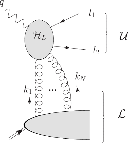
In this paper we restrict our attention to contributions from graphs of the form of Fig. 1(a), and it will be most convenient to work at the level of the amplitude shown in Fig. 2. The upper part of the graph, denoted by , describes the scattering of a virtual photon off gluons. The lower part of the graph, denoted by , describes the emission of the gluons from the target proton. In general, the amplitude for scattering off gluons in the target can be conveniently expressed as the contraction of and . With the momentum labels shown in Fig. 2, we have
| (4) |
Here runs from to . We will use to label the electromagnetic index, and to label the gluon indices. The quark and anti-quark momenta are and and emerge from the hard scattering at wide angles. The label the gluons connecting the two subgraphs. We will be examining the contribution when each is in a neighborhood of the target collinear region:
| (5) |
We can treat both and as being obtained by a sum over all graphs with the requisite external lines. From the examination of examples, it can be seen that each graphical contribution to the amplitude is obtained times. We compensate by defining to include a factor .
III Simplest Case: A Single Target Gluon
 |
 |
| (a) | (b) |
We start with the simple case of the exchange of one gluon, as shown in the graphs of Fig. 3. The amplitude is of the form
| (6) |
The subscript denotes that one gluon is exchanged, and we have explicitly shown the numerator of the gluon propagator. To simplify notation, we will often omit the momentum arguments and the index of the electromagnetic current.
The gluon is collinear to the target, and and are at wide angle, so that the quark subgraph is the hard scattering. We will show that, after a sum over diagrams, the lower part of the graphs in Fig. 3 can be separated into a factor that can be identified as a contribution to the gluon distribution function.
There are regions where the target gluon may go far off-shell, but in that case it should be regarded as belonging to the hard-scattering subgraph at one higher power of . For this paper, we restrict ourselves to the case where the hard-scattering coefficient is lowest order (LO) in .
III.1 Power counting
To understand the power counting in , for large , we first observe that the target is highly boosted in the plus direction, so that
| (7) |
up to an overall power of . Since and are at wide angles, all components of are of comparable size, and given by the dimension of the quark part of the graph:
| (8) |
To obtain the structure function, we square the amplitude and integrate over the final states. The integral over the gluon momentum is invariant under boosts from the target rest frame, and therefore does not contribute any power of . The Lorentz-invariant phase space integral for the pair,
| (9) |
is dimensionless. Thus it also contributes a zero power of when the quark-antiquark pair is at a wide angle, where all components of and are of order . Thus the overall power of is that for the squared amplitude.
From Eqs. (7), (8), we see that the largest power of is from the term , for individual graphs. Squaring this gives the previously mentioned super-leading power of in a structure function. In the next subsection, we will use a generalizable method to demonstrate cancellation of the super-leading terms in the amplitude. To give a correct treatment of the leading terms (), we need to work at next-to-leading power accuracy in relative to the super-leading power. We also need to show that the leading terms correspond to a correct definition of the gluon density.
III.2 and gluons
A convenient technique was introduced by Grammer and Yennie in the context of QED [8]. In this approach, the propagator numerator in Eq. (6) is split into two parts:
| (10) |
where
| (11) | ||||
| (12) |
In these definitions, we use the light-like direction which characterizes the outgoing jet direction. The rationale for this choice is that the dominant term in is the one obtained from the component of the gluon-propagator numerator. reproduces exactly this component, the remaining components of give smaller contributions, and has a factor , which allows gauge invariance to be applied.
We use Eq. (10) to separate Eq. (6) into two parts which we call the “-term” and the “-term.” We will also use the terminology of the exchange of “-gluons” and “-gluons”.
From Eq. (5), we determine the dependence that results from the individual components in the -term:
| (13) | ||||
| (14) | ||||
| All others | (15) |
The term gives the super-leading contribution, associated with the power of in . Changing to removes one power of , by changing to . The resulting power, , we identify as the standard leading behavior.
As we will see explicitly, gauge invariance ensures that dotted into the sum of all graphs in the upper bubble vanishes, so that
| (16) |
Hence the -term can be dropped, so that Eq. (6) gives
| (17) |
Only the terms with transverse components on are unsuppressed in Eq. (17). This is easily verified by defining
| (18) |
and recalling Eqs. (5), (7). Checking each combination of indices we find,
| (19) | ||||
| (20) | ||||
| (21) |
Therefore, the transverse term dominates, and the other terms are power suppressed or zero.
III.3 Gauge-invariance calculation
We now give an explicit demonstration that . The graphs of Fig. 3 give
| (22) |
Then for the -term we have
| (23) |
to which we apply the following identities for :
| (24) | ||||||
| (25) |
Using the Dirac equation for and , we find that two terms vanish and the remaining terms exactly cancel, so
| (26) |
Therefore, only the -term survives, so that
| (27) |
We now have the power-counting of Eqs. (19)–(21). It is important to recognize that we wrote the amplitude in the form of Eq. (27) without making any approximations. It is very tempting to replace by an exactly collinear value at the start of the argument, both in the upper, hard-scattering subgraph, and in Eqs. (11) and (12). The approximated momentum is on-shell and has zero transverse momentum. This replacement is particularly natural to make in the term, and was made by Labastida and Sterman [5]. However, then we would have made an error in each graph contributing to the -term that is of order relative to the super-leading power . That is, the error would be of the same order as the leading terms in the final result. Using this kinematic approximation in the term also entails using it in the term, and we would not have obtained the contribution to involving the transverse components of . If we make the collinear approximation in the upper subgraph but not in , then the cancellation of the -terms in Eq. (23) is no longer exact. (The error would again be of order relative to the super-leading power.) These observations will be particularly important for obtaining the correct two-gluon contribution in Sect. V.
III.4 Leading-power Factorization
The next step in obtaining the factorization formula for scattering off a single target gluon is to drop power-suppressed terms. This means we can drop the contribution from Eq. (20) and keep only the sum over transverse components in Eq. (27). Furthermore, since we are restricting to the region of given by Eq. (5), we can now substitute the approximate parton momentum,
| (28) |
into the upper bubble only. Thus the hard scattering is initiated, as is usual, by a massless on-shell parton of zero transverse momentum. The amplitude is then
| (29) |
where the index runs only over the two transverse components. In an unpolarized cross section or structure function, we square the amplitude and sum/integrate over final states. However, we have assumed above that the outgoing quarks are at wide angles, so that the collinear approximation (28) for the gluon can be safely applied in the upper part of the graphs.
But in the integral over all final states, there is also a leading contribution from the region where one of the intermediate quark lines is collinear to the target, i.e., or . This contribution to the cross section is already taken into account at the parton-model level, and therefore an appropriate subtraction should be made to avoid double counting, according to the principles summarized in the Appendix. Thus the contribution of the graphs to the structure tensor takes the form
| (30) |
Here, denotes the complete integration measure including sums over final states. The exact form of the subtraction terms is found by making the parton-model approximation on the struck quark, appropriate for the region of phase space where one of the quarks is target collinear. (The detailed steps for making this approximation are reviewed in the introductory sections of Ref. [9].) We denote the parton-model approximation on the upper part of the graph by . Furthermore, in the sum over final states for the unpolarized cross section, is diagonal in and , so we may write Eq. (30) as,
| (31) |
where . We note that the manipulations needed to obtain Eq. (31) can be made transparent by first writing the contractions of the upper and lower bubbles in terms of sums over transverse polarizations:
| (32) |
where we have introduced transverse polarization vectors,
| (33) |
Then by the use of diagonality of after the integral over the final state, the sums over polarizations produce Eq. (31).
The first factor in the integrand of Eq. (31) is just the unpolarized squared amplitude for scattering minus a subtraction term. For the rest of this paper, we will ignore the details of implementing the double counting subtraction since it only modifies the hard scattering but does not affect Ward identity arguments such as those of Sect. III.3.
Since depends only on the plus component of after the approximation of Eq. (31), the integration over and depends only on the target bubble. Thus, we will ultimately identify the lowest order contribution to the gluon PDF with the factor,
| (34) |
where represents a general sum/integral over the final states of the target bubble, and the factor gives the standard normalization for the gluon density. The factorization formula that follows from Eq. (31) can thus be expressed graphically as
| (35) |
The upper part of the graph now has the interpretation of an on-shell scattering amplitude for a virtual photon to scatter off a transversely polarized gluon with exactly collinear momentum. In a general treatment of factorization, the steps of this section need to be generalized to more than one gluon, and factors like Eq. (34) need to be shown to correspond to an operator definition of the gluon distribution function. Therefore, before we go further we must examine the general properties of the gluon distribution function.
IV The Gluon Distribution Function
IV.1 Operator Definition
For Eq. (35) to be a consistent factorization formula for the single-gluon case, Eq. (34) should correspond to the relevant contribution to the operator definition of the gluon PDF. The standard definition [6] of the integrated momentum space gluon distribution function for the proton is
| (36) |
Here is the longitudinal momentum fraction of the proton carried by the target gluon. To make the definition exactly gauge invariant, we have inserted a Wilson line operator in the adjoint representation,
| (37) |
where the () are the generators of SU(3) in the adjoint representation and is the path-ordering operation. The are related to the structure constants, , by . The color indices of are contracted with those of the gauge field-strength tensor, whose definition we recall:
| (38) |
Then examining how to apply Eq. (36) in perturbative calculations yields Feynman rules for the gluon PDF. In perturbative calculations, it is convenient to substitute the following identity for the Wilson line operator,
| (39) |
and to insert a complete sum over final states. Then Eq. (36) becomes
| (40) |
The symbol includes all sums and integrals over final states. Expanding the Wilson line in small coupling gives the relation,
| (41) |
The Feynman rules for the gluon PDF are found by using Eqs. (41), (38) inside Eq. (40) and directly applying the rules of ordinary perturbation theory.
IV.2 Lowest Order
We now expand the operators in Eq. (40) in powers of . At zeroth order, only the derivative terms in Eq. (38) contribute to Eq. (40):
| (42) |
Directly applying the rules of perturbation theory yields
| (43) |
where the factors and denote the parts of the incoming target bubble to the left and right of the final-state cut, with their color indices. Equation (43) is exactly what we asserted to be the gluon-density factor, Eq. (34), for DIS with a single target gluon. To express Eq. (43) diagrammatically, we define the following Feynman rules: There is a lower bubble representing the incoming target,
| (44) |
For the factors in Eq. (43) we use the notation
| (45) |
Since Eq. (45) modifies the vertex to the gluon from the target bubble in Eq. (43), we refer to it as the “special” vertex. Diagrammatically, we notate the contribution to the gluon PDF from a single gluon emission on each side of the cut as
| (46) |
Implicit in this notation are an overall factor of , integrals of and , and a sum over the gluon color index . Then Eq. (35) can be written as
| (47) |
IV.3 Beyond Lowest Order
General Feynman rules for the gluon PDF, Eq. (36), are found [6] by keeping other terms in the expansion of the Wilson line operator, and the third term in Eq. (38). To start out, let us ignore the third term in Eq. (38). Looking only at the operators on one side of the final-state cut and using Eq. (41), we get factors in the integrand of the form
| (48) |
At this order of perturbation theory, gluons are emitted from the target bubble, with color indices .
Now we treat the contributions which use the third term in the field-strength tensor Eq. (38). To stay at the same order of perturbation theory as in (48), we must drop down one order in the expansion of the Wilson line operator. Thus, we obtain contributions of the form
| (49) |
Rather than treating the derivative terms and the third term in Eq. (36) separately, we can combine (48) and (49) at each order of perturbation theory. The complete contribution is then
| (50) |
The first factor in (50) tells us what the special gluon vertex analogous to Eq. (45) is for gluons. It differs from the corresponding factor in (48) by having the gluon momentum replaced by the total momentum in the first term only. We therefore obtain the Feynman rules for the gluon PDF shown in Fig. 4, where factors and on the left and the right of the final-state cut have been dropped, and we have removed a factor of , just as in Eq. (45). A general contribution to the gluon PDF is illustrated in Fig 5. To simplify expressions, in later sections we will drop the explicit appearance of in the eikonal denominators.
 |
 |
 |
| (a) | (b) | (c) |

V Scattering Off Two Collinear Gluons
We now extend the treatment of Sect. III to the case of two target-collinear gluons. The graphs under consideration are shown in Fig. 6. Our aim is to show that when the graphs are summed, Ward identities similar to what were used in Sect. III lead to a factorized structure. For a consistent factorization formula, the resulting gluon PDF should correspond to what is obtained using the Feynman rules of Fig. 4.
 |
 |
 |
| (a) | (b) | (c) |
 |
 |
 |
| (d) | (e) | (f) |
V.1 Power counting and , decomposition
As in the previous sections, we write the amplitude obtained from the graphs in Fig. 6 as the contraction of an upper part and a lower part, connected by gluon-propagator numerators:
| (51) |
All incoming gluons are target collinear, with the sizes of the momentum components given in Eq. (5). The gluons have leading contributions from regions where they are far off-shell, but these contribute only at high order in . Furthermore, since there are only gluon-fermion couplings in the upper part of the graph, ghosts do not enter at this level of the calculation. A general, all-orders proof will need to take into account ghost attachments as well.
The upper part has one more external gluon than before, so its dimension is reduced by a single power of ; all the components of are therefore to be treated as order . The lower bubble now includes two Lorentz indices, and in the boosted frame has, up to overall powers of order , the power dependence,
| (52) | ||||
| (53) | ||||
| (54) | ||||
| (55) | ||||
| (56) |
Combined with the factor from , this gives a super-leading contribution from the components, leading contributions from the and components, and power-suppressed contributions from the other components.
That the term gives a superleading result is an example of a general result from power-counting arguments: A superleading contribution arises whenever all the gluons joining the collinear and hard subgraphs are longitudinally polarized. We will show that there is a cancellation after a sum over all graphs for leaving a result that is just leading power. That there is a leading contribution from the and terms is expected: They correspond to a hard scattering on a transversely polarized gluon accompanied by a longitudinally polarized gluon. The remaining terms are of a non-leading power, and we can therefore ignore them. We will show that after a sum over graphs, the total of the , and terms is equivalent at leading power to a hard scattering off a single transversely polarized gluon multiplied by the appropriate two-gluon factor obtained from the Feynman rules for the gluon PDF.
Just as with the single-gluon case, we split the propagator numerators into and terms:
| (57) | ||||
| (58) |
where , , and are defined just like , , except for the replacement of by the appropriate gluon momentum, or . So we write Eq. (51) as
| (59) |
Exactly as in the previous section, the term gives a super-leading contribution, graph-by-graph, while the and terms are leading. The term is power suppressed, and so we neglect it. Each of the non-suppressed terms has a factor of or , so we will next apply gauge invariance to get a result of the general form
| (60) |
The first factor is just the basic amplitude already considered in the previous section, but with gluon momentum :
| (61) |
The remaining factor will determine what “special” vertex, analogous to Eq. (45), we should use for the gluon density.
V.2 Gauge invariance on factor
We first apply the method of Sec. III.3 to a single -gluon in Eq. (59). The explicit expression for the upper bubbles in the first three graphs in Fig. 6 is
| (62) |
We organize these graphs by having the gluon attached in one place on the quark line, and then the graphs correspond to the different possible placements of the gluon. Similarly, for the other three graphs,
| (63) |
In Eq. (59), the terms that are leading or super-leading have at least one -gluon, to which we apply the method of Sec. III.3. We start with the case of any term involving . For graphs (a)–(c), we have a factor
| (64) |
Calling the terms in brackets term 1, term 2, and term 3, we now make use of the following identities:
| (65) | ||||||
| (66) | ||||||
| (67) |
Using the Dirac equation to eliminate two of the terms, we then have
| (68) |
The last two terms cancel because of the Abelian nature of the QED coupling. However, the remaining terms lead to a non-vanishing result due to the non-vanishing commutation relations for and ,
| (69) |
Similarly for graphs (d)–(f) we have
| (70) |
Adding Eqs. (69) and (70), we get
| (71) |
This is the general expression for the upper bubble when it is contracted with the -term from gluon 2. Notice that it vanishes when the theory is Abelian. This is an example of a general result that -gluons give zero contribution in an Abelian gauge theory. Notice also that it is of the form of the upper factor (22) for one gluon of momentum , times an eikonal factor.
V.3 Gauge invariance on factor
If we instead consider the contraction of the upper bubble with the gluon from gluon 1, then exactly similar steps lead to,
| (72) |
Note the overall minus sign that arises from the reversed roles of gluon 1 and gluon 2. To complete the analysis, we must consider the separate cases: where the other gluon is also a -gluon, or where one gluon is a -gluon and the other is a -gluon.
V.4 term
The term in Eq. (59) follows immediately from Eq. (71) when we include the contraction with :
| (73) |
This has the form of the amplitude (22) with a single gluon of momentum multiplied by a special vertex. Thus for the term in Eq. (59), we have:
| (74) |
The two -gluons have been factored out into eikonal couplings. A diagrammatic representation of Eq. (73) is shown in Fig. 7. Note that this term would exactly vanish in an Abelian theory, where .

Graph-by-graph, this is still super-leading, since the factor of and everything to its right power-counts just like for the case of one-gluon exchange. Furthermore, (74) is not symmetric between the gluon momenta, and , despite the symmetric occurrence of and factors on the left-hand side. Both problems are remedied by applying the decomposition to the factor in Eq. (74):
| (75) |
where
| (76) | ||||
| (77) |
The term gives zero when multiplied with (see the calculation in Sect. III.3). This removes the super-leading part, just as in one-gluon exchange, leaving only the term. Hence, the term is
| (78) |
Thus it has the structure of Eq. (60).
V.5 term
V.6 term
For the term we similarly obtain
| (80) |
Note the overall minus sign relative to Eq. (79) that arises because of the reversed role of gluons 1 and 2. A graphical representation of the factorization in Eqs. (79) and (80) is shown in Fig. 8.
 |
| (a) |
 |
| (b) |
V.7 Factorization and the Gluon Distribution Function
Adding Eqs. (78), (79), and (80) gives
| (81) |
This may be written compactly if we define the factor in braces to be
| (82) |
Normally a vector like this would have its component power counting as . In fact this component is zero. The reason is that it is constructed from a combination of , , and , each of which gives this property individually.
The importance of the last remark is that it shows that the dominant contribution, i.e., the leading-power contribution, is from transverse values of , so that , which goes into the hard-scattering factor, can be treated as having an incoming transversely polarized gluon. Compare this with what is found in Eq. (29).
It is the factor which we would like to identify with a two-gluon factor in the amplitude for the gluon distribution function. The derivation so far, where we have systematically eliminated super-leading contributions, shows that we have a result with the standard leading power of , i.e., . The leading terms are for , a transverse index:
| (83) |
The steps for obtaining a factorization formula are now exactly analogous to the steps in Sect. III.4. The analogue of Eq. (29) for the case of two gluons is
Here we have defined .
The factor , given in Eq. (83), is exactly what is obtained from the Feynman rules for the gluon PDF listed in Fig. 4. This would not have happened if we had neglected the contribution from Sect. V.4 to the leading behavior in Eq. (83). Equation (78) is therefore important for agreement between the Feynman rules for the gluon density and the leading contribution to DIS.
To summarize this section, we find that leading-power contributions arise when one or both gluons is longitudinally polarized. With one longitudinally polarized gluon, we get expected eikonal factors in Eqs. (79,80), after a sum over graphs. These factors are analogous to the eikonal propagators that appear in the quark PDF, but they do not have the correct Feynman rules to correspond to the gluon PDF. A further contribution Eq. (78) arises when both gluons are longitudinally polarized. Previously, this contribution was expected to vanish (see, e.g., [5]). But it is in fact non-vanishing, and is needed for a correct correspondence with the definition of the gluon PDF.
VI Summary and Conclusion
We have given a direct illustration using gluon-induced DIS that contributions from longitudinally polarized gluons do not cancel in sums over graphs in Feynman gauge. Indeed, they yield leading contributions that are needed to correctly identify the standard gluon PDF. Calculations that go beyond lowest order in therefore require care in how the polarization of external gluon lines is treated, and involves keeping appropriate combinations of - and -terms in a Grammer-Yennie style treatment. Although we have obtained our result for the simple case of the integrated PDF, our arguments relied only on the application of Ward identities at the amplitude level. Therefore, similar results should hold for unintegrated PDFs (and related objects like fragmentation functions) once suitable definitions have been established. Since Eq. (74) exactly vanishes in an Abelian theory, this result is a specific example of how the non-Abelian nature of QCD can complicate factorization arguments.
Higher-order calculations of hard-scattering coefficients involve subtraction terms with multiple target-collinear gluons, so the results obtained here are of direct importance for obtaining correct hard-scattering coefficients beyond lowest order consistent with factorization and a well-defined gluon PDF.
Standard power-counting shows that it is also possible to get leading contributions when the hard scattering is induced by Faddeev-Popov ghosts, but only at higher order in the hard scattering than is treated in this paper. It is natural to expect a generalization of the known results [10, 11] for the operator product expansion that applies to moments of DIS structure functions. On this basis we expect the general result to be that the sum over all graphs gives extra contributions to the factorization properties involving coefficients times what we will call alien PDFs. The operators defining the alien PDFs are variations of certain parent operators under Becchi-Rouet-Stora-Tyutin transformations and therefore vanish in physical matrix elements. Non-vanishing of the Green functions of the alien operators with off-shell quark and gluon states has caused calculational problems [12, 13].
Acknowledgments
We thank A. Stasto and G. Sterman for useful conversations.
Feynman diagrams were made using JaxoDraw [14]. This work was supported by the U.S. D.O.E. under grant number DE-FG02-90ER-40577.
Appendix A Subtractions
We now review the subtractive approach — e.g., [15] and Sect. VI of [9] — we use for determining the hard-scattering factorization. It is generalized from the Bogoliubov approach to renormalization. Our strategy is to recursively examine successively larger leading regions for the DIS cross sections.


The procedure starts with a handbag-diagram structure — Fig. 9 — to give the LO term, i.e., the parton-model formula. This term is obtained by an approximation valid to leading power when the incoming quark is nearly on-shell and collinear to the target. The approximation is denoted by the hooked line in Fig. 10, and it involves replacing the momentum of the struck quark in the upper part of the graph by its parton-model approximation, which is massless, on-shell, and of zero transverse momentum.
If a general graph contributing to the cross section is denoted by , then we call graphs where we make the parton-model approximation . At this level we also need to consider graphs with arbitrarily many target-collinear gluons attaching to the the hard vertex — Fig. 11. A Ward identity allows the target-collinear gluons to be disentangled from the LO hard-scattering coefficient. Since there are no super-leading contributions in these graphs, and since the relevant graphs are tree graphs, the Ward identities are unproblematic.
The result is a convolution product of the LO hard-scattering coefficient with a sum of graphs identifiable as an expansion of the quark PDF. Schematically, the cross section is then written,
| (88) |
where is the quark PDF, is the LO hard-scattering coefficient (from the electromagnetic vertex), and symbolizes the usual convolution product.
Some of the errors in this approximation are power suppressed, indicated by the term where , and we do not consider them further. Other errors are caused by regions with larger transverse momentum for the quarks and gluons, and by graphs not of the form of Figs. 9 and 11. These will be covered by our treatment of higher-order scattering, and are suppressed only by a power of the strong coupling at scale , as indicated by the term .
Hence, we have the LO approximation to the DIS cross section
| (89) |
 |
 |
|---|---|
| (a) | (b) |
To find the next-to-leading (NLO) contribution, we examine, among others, graphs of the topologies shown in Fig. 12. Specific examples are included in the graphs we treat in the main body of the paper. For the moment we ignore the possibility of extra gluon exchanges. Some of the graphs, e.g., Fig. 12(a), are among those already considered in the LO approximation, merely viewed with a different partition between the lower bubble and the parton lines explicitly drawn at the top.

Therefore, before we can get the true NLO contribution, we must first subtract the LO approximation:
| (90) |
This is just the remainder from applying the approximation already considered in Eq. (88). Finally, to evaluate Eq. (90), we apply approximations that are good for the wide-angle parton subprocesses, denoted by the symbol :
| (91) |
where we must now allow for a sum over parton flavors. For the graph in Fig. 12(a), the result is shown graphically in Fig. 13.

If graphs like Fig. 12(a) were all that mattered, then this would complete the discussion of the subtraction formalism. However, the gauge-invariant LO term needs a generalized handbag structure including extra gluon exchanges, as in Fig. 11. There are thus corresponding subtractions for graphs like Fig. 12(b), as shown in Fig. 14. Implementing the appropriate approximations and applying Ward identities allows us to identify how the second term in Fig. 14 contributes at LO. After applying Ward identities, the second term in Fig. 14 can be written diagrammatically as in Fig. 15. There we see the separation of the graph into the LO hard-scattering matrix element and a single-gluon contribution to the PDF.
Thus we see that evaluating Eq. (91) for the NLO correction requires that we know exactly the single-gluon correction to the quark PDF in Eq. (89), since the definition of the approximation is what gives us the lowest order, parton-model factorization in Eq. (88). In other words, using the subtraction approach to calculate higher-order corrections to the hard-scattering coefficient requires that we know exactly what we are subtracting.

References
- [1] J. C. Collins, D. E. Soper and G. Sterman, Nucl. Phys. B 261, 104 (1985); J. C. Collins, D. E. Soper and G. Sterman, Nucl. Phys. B 308, 833 (1988).
- [2] G. T. Bodwin, Phys. Rev. D 31, 2616 (1985) [Erratum-ibid. D 34, 3932 (1986)].
- [3] J. C. Collins, Phys. Lett. B 536, 43 (2002) [arXiv:hep-ph/0204004].
- [4] S. J. Brodsky, D. S. Hwang and I. Schmidt, Phys. Lett. B 530, 99 (2002) [arXiv:hep-ph/0201296].
- [5] J. M. F. Labastida and G. Sterman, Nucl. Phys. B 254, 425 (1985).
- [6] J. C. Collins and D. E. Soper, Nucl. Phys. B 194, 445 (1982).
- [7] C. Ewerz, A. von Manteuffel and O. Nachtmann, Phys. Rev. D 77, 074022 (2008) [arXiv:0708.3455 [hep-ph]].
- [8] G.J. Grammer and D.R. Yennie, Phys. Rev. D 8, 4332 (1973).
- [9] J. C. Collins, T. C. Rogers and A. M. Stasto, Phys. Rev. D 77, 085009 (2008) [arXiv:0708.2833 [hep-ph]].
- [10] S. D. Joglekar and B. W. Lee, Annals Phys. 97, 160 (1976).
- [11] M. Henneaux, Phys. Lett. B 313, 35 (1993) [Erratum-ibid. B 316, 633 (1993)] [arXiv:hep-th/9306101].
- [12] J. C. Collins and R. J. Scalise, Phys. Rev. D 50, 4117 (1994) [arXiv:hep-ph/9403231].
- [13] B. W. Harris and J. Smith, Phys. Rev. D 51 4550 (1995) [arXiv:hep-ph/9409405].
- [14] D. Binosi and L. Theussl, Comput. Phys. Commun. 161, 76 (2004) [arXiv:hep-ph/0309015].
- [15] J.C. Collins, Phys. Rev. D 65, 094016 (2002) [arXiv:hep-ph/0110113].