TIT/HEP–581
TU–813
UT-08-06
May, 2008
Intersecting Solitons
Amoeba
and Tropical Geometry
Toshiaki Fujimori1,
Muneto Nitta2,
Kazutoshi Ohta3,
Norisuke Sakai4
and
Masahito Yamazaki5
1Department of Physics, Tokyo Institute of
Technology
Tokyo 152-8551, JAPAN
2Department of Physics, Keio University, Hiyoshi,
Yokohama, Kanagawa 223-8521, JAPAN
3Department of Physics,
Tohoku University, Sendai 980-8578, JAPAN
4Department of Mathematics, Tokyo Woman’s Christian University,
Tokyo 167-8585, JAPAN
5Department of Physics, University of Tokyo, Tokyo 113-0033, JAPAN
Abstract
We study generic intersection (or web) of vortices with instantons inside, which is a 1/4 BPS state in the Higgs phase of five-dimensional supersymmetric gauge theory on with Higgs scalars in the fundamental representation. In the case of the Abelian-Higgs model (), the intersecting vortex sheets can be beautifully understood in a mathematical framework of amoeba and tropical geometry, and we propose a dictionary relating solitons and gauge theory to amoeba and tropical geometry. A projective shape of vortex sheets is described by the amoeba. Vortex charge density is uniformly distributed among vortex sheets, and negative contribution to instanton charge density is understood as the complex Monge-Ampère measure with respect to a plurisubharmonic function on . The Wilson loops in are related with derivatives of the Ronkin function. The general form of the Kähler potential and the asymptotic metric of the moduli space of a vortex loop are obtained as a by-product. Our discussion works generally in non-Abelian gauge theories, which suggests a non-Abelian generalization of the amoeba and tropical geometry.
1 Introduction
The study of topological solitons is intimately connected with the development of mathematics. Originally solitons are found as solutions to non-linear (field) equations in various physical systems, but many mathematical concepts have been developed at the same time in order to understand properties and integrability of the soliton equations. Indeed, many mathematical tools, such as representation theory of differential operator algebra and infinite dimensional Grassmannian, are required to investigate the solitons. The language of two-dimensional conformal field theory is also useful in studies of a class of the soliton systems, such as KdV, Toda, KP equations. The investigation of solitons in gauge theory, such as instantons and monopoles, gives not only non-perturbative informations about the field theory, but also stimulates new developments of differential geometry.
The purpose of the present article is to study topological solitons using novel mathematical objects known as amoeba and tropical geometry. We find a one-to-one correspondence between amoeba/tropical geometry and solitons in Yang-Mills-Higgs theory. Yang-Mills gauge fields coupled to the Higgs fields naturally appear as a bosonic part in supersymmetric Yang-Mills theory with eight supercharges. When sufficient number of the Higgs fields get vacuum expectation values (vevs), the theory is in the Higgs phase with completely broken gauge symmetry. Typical solitons in the Higgs phase known for a long time are vortices in the Abelian gauge theory coupled to a single complex Higgs field (the Abelian-Higgs model) [1]. These vortices have been recently extended to the non-Abelian case, vortices in completely broken non-Abelian gauge symmetry [2]–[12]. The other fundamental solitons found relatively recently in Yang-Mills-Higgs theory (or corresponding nonlinear sigma models) are domain walls or kinks [6], [13]–[16]. Since both vortices and domain walls preserve half of the supercharges when embedded into supersymmetric theories, they are called 1/2 BPS solitons. Composite solitons in the Higgs phase have recently been studied extensively, especially in supersymmetric gauge theories with eight supercharges [17, 18, 19]. Since the magnetic field has to vanish in the Higgs phase, magnetic monopoles are confined by vortices (confined monopoles) [20]–[23]. Although isolated instantons shrink to points in the Higgs phase, they can lie inside a vortex core (trapped instantons) [22, 23]. Vortex-strings can end on a domain wall [24] or stretch between domain walls [25]. When a (composite) soliton configuration breaks directions of translational symmetry, it is defined to have codimensions. The composite soliton with the lowest co-dimension is a web or a network of domain walls, whose moduli space and dynamics have been worked out recently [26]-[30]. All of these composite solitons preserve 1/4 of supercharges if we realize the Yang-Mills-Higgs theory as a supersymmetric Yang-Mills theory, and are called 1/4 BPS states. It has been found that all these 1/4 BPS composite solitons are related by the (Scherk-Schwarz twisted) dimensional reduction, starting from the instanton-vortex system [23]. Therefore understanding the instanton-vortex system is of primary importance to study BPS solitons in supersymmetric Yang-Mills-Higgs theories with eight supercharges.11 1 It is worth pointing out that there exist the other series of 1/4 BPS systems. This contains a triple intersection of vortices where a set of two vortices has one common codimension [31], contrary to the instanton-vortex system [23] where vortices have no (or two) common codimensions. The former preserves (1,1) SUSY and the latter (2,0) SUSY in terms of two-dimensional supersymmetry [32]. Different sets of 1/4 BPS equations in these two series are obtained as dimensional reductions of the unique set of the 1/8 BPS equations [32, 33]. Unfortunately, generic configurations of instantons and vortex sheets as co-dimension four solitons have not been worked out, apart from a trapped instanton as a lump on a (uncurved) vortex plane, or an intersection point of two orthogonal (uncurved) vortex planes [23]. It is important to characterize generic configurations of instantons and vortex sheets as co-dimension four solitons in a precise and transparent manner. We can call these solitons as webs of vortices. We show that these soliton webs are nicely described in terms of the amoeba and the tropical geometry.
Interestingly, amoeba and tropical geometry have already appeared in physics literature, in the context of topological strings. Topological string amplitude (or its building block, topological vertex) can be described by means of a melting crystal picture [34, 35], which was originally introduced as a statistical model in mathematical physics. Shape of the melting crystal in the thermodynamic limit is well interpreted in terms of an amoeba, which is a logarithmic projection of a smooth Riemann surface. On the other hand, an emaciated body of the amoeba corresponding to zero temperature limit can be captured by tropical geometry, where we can obtain some properties of the Riemann surface from a skeleton of the amoeba. In the context of superstring theory, the amoeba and tropical geometry appear as, respectively, quantum () and classical () shape of intersecting five-branes (five-brane junctions), which are dual to a suitable Calabi-Yau geometry where the topological string is defined. Other examples appear in an instanton and BPS state counting problem of the supersymmetric (quiver) gauge theories [36, 37, 38], since these systems are closely related to the topological string amplitudes and realized in terms of the five-brane web.
The five-brane system is useful to understand the relationship between the gauge and string theory, and the amoeba and tropical geometry, which is the main subject of this article. Our study is inspired by these successful applications of the amoeba and tropical geometry to physics. We find a similarity between the five-brane web and the 1/4 BPS composite solitons of vortex sheets and instantons. Some of properties of the webs of vortices are still unclear. In particular, the instanton charge appears at the intersection point of the vortices, but we have not obtained a tool to see a distribution of the extra instanton charge on the vortex web. The five-brane web in the superstring theory and vortex web possess common properties. Indeed, toric diagrams and geometry play an important role in both sides, and their moduli spaces are described by similar quotient spaces and the moduli space of the vortex web should be included in that of the five-brane web. So we expect that the amoeba and tropical geometry, which is important to understand dynamics of the five-brane web, are also useful to analyze the web of the solitons in the Yang-Mills-Higgs system.
In this paper, we study the most generic configurations of 1/4 BPS solitons of instantons and vortices in the Higgs phase of the five-dimensional supersymmetric gauge theory (with eight supercharges) on with Higgs scalars in the fundamental representation, by using the moduli matrix formalism [18]. Torus allows us to obtain other 1/4 BPS solitons readily through dimensional reduction. We show that vortex sheets are defined by zeros of a Laurent polynomial of two complex coordinates of , and instanton positions are given by common zeros with another polynomial. We find that the above expectation of the importance of amoeba and tropical geometry to be correct. We describe physical quantities of the intersecting solitons (soliton web) in terms of the mathematical language of amoeba and tropical geometry. We also see the important objects in the amoeba and tropical geometry, such as the logarithmic mapping, the Ronkin function and the Monge-Ampère measure, also have essential meanings on the soliton side. We describe properties of the soliton web in terms of these mathematical objects. We find that the moduli matrix approach is very useful in the translation between physical and mathematical languages.
The organization of the present paper is as follows. In Sec. 2, we review the 1/4 BPS equations for vortices and instantons in the Higgs phase of five-dimensional supersymmetric gauge theory on with Higgs scalars in the fundamental representation, using the moduli matrix formalism. We mainly consider vortices in the overall gauge theory except in Sec. 5. In Sec. 3, we consider simpler case of vortex on cylinder . In Sec. 4, we study the most general situation of vortex sheets on . Sec. 4.1 gives amoeba corresponding to vortex sheets. Sec. 4.2 relates it to the tropical geometry and gives an example. Sec. 4.3 describes a general formula to compute the topological charges. Sec. 4.4 gives the metric of the moduli space of a vortex loop. We also obtained a new general formula for the Kähler metric which is valid for arbitrary values of and . In Sec. 5, we examine the instanton number in non-Abelian gauge theory. Sec. 5.1 reviews the instanton number for instantons trapped inside a non-Abelian vortex plane [23]. Sec. 5.2 discusses more general configurations of the instantons trapped inside a non-Abelian vortex web. Sec. 6 is devoted to conclusion and discussion.
2 Vortices and Instantons
In this section, we first review the construction of vortex solutions in gauge theory in (4+1)-dimensional spacetime with Higgs fields in the fundamental representation. By introducing additional Higgs fields in the fundamental representation, this theory can also be regarded as the bosonic part of a five-dimensional supersymmetric gauge theory with hypermultiplets in the fundamental representation, but the fermionic part (and another set of Higgs scalars) is irrelevant and is omitted in the following discussion. We introduce and as real and complex coordinates of , respectively.
The Lagrangian of the theory takes the form
| (2.1) |
where the Higgs fields are expressed as an matrix . The covariant derivative is defined by and the field strength by . The constants and are the gauge coupling constant and the Fayet-Iliopoulos (FI) parameter, respectively. At the vacua (the minima of the potential) of this theory, the Higgs fields get vev and gauge symmetry is completely broken. Namely the theory has only the Higgs branch due to the nonzero FI term. The moduli space of the vacua is given by a complex Grassmannian
| (2.2) |
Considering a static gauge configuration, we find that there is a lower bound of the energy [22, 23]
| (2.3) |
where the two form is the Kähler form on , and we have defined the total instanton charge as an integral of the instanton charge density , and the vortex charge as a divergent integral of the vortex charge density
| (2.4) | |||||
| (2.5) |
The lower bound Eq. (2.3) is saturated if the following BPS equations [22, 23]
| (2.6) |
are satisfied. When FI parameter is sent to zero, the Higgs field vanishes and these equations reduce to the anti-self-dual equations for Yang-Mills instantons, whereas when we neglect the -(or -)dependence of the fields they reduce to simple vortex equations for vortices on the -(or -)plane. These vortices are two-codimensional surfaces in the four dimensional space . Therefore the BPS equations (2.6) contain at least instantons and intersecting vortex sheets. As we will see below, these equations describe webs of vortex sheets in general. The equations (2.6) were earlier found for those on arbitrary Kähler manifold [39] and were simply called ‘‘vortex equations” although they contain instantons also.22 2 In Ref. [39] the vortex equations are defined on arbitrary Kähler manifold of complex dimension (with not necessary). There the bound is given by and with the Kähler 2-form , instead of the charges (2.4) and (2.5). Furthermore at least in the case of these generalized equations can be obtained as equivariant dimensional reduction of the Donaldson-Uhlenbeck-Yau equations on with a monopole configuration on [40]. It has been shown in [23] that solutions to the BPS equations (2.6) on (or ) preserve a quarter of supercharges in the supersymmetric gauge theory with eight supercharges. So the configuration of the solution is called a 1/4 BPS state in this sense. The energy of the BPS configuration is determined by the topological charges (2.4) and (2.5).
The vortex charge can be evaluated from the sum of the area of each vortex sheet, as we will see in Sec. 4. The total instanton charge can be decomposed into the intersection charge and the instanton number as
| (2.7) | |||
| (2.8) | |||
| (2.9) |
The intersection charge has negative contribution to the energy of the BPS configuration, which can be regarded as binding energy of intersecting vortex sheets. On the other hand the instanton number (not to be confused with total instanton charge) counts to the number of usual (particle-like) instantons and has positive contribution to the energy.
Let us solve the BPS equations (2.6). The first BPS equation in (2.6) is equivalent to an integrability condition33 3 If we identity the Higgs field as a set of sections of a rank vector bundle on the base Kähler manifold, then the first BPS equation is equivalent to the condition of the existence of the holomorphic frame , which satisfy . for the differential operators , which states that there exists an matrix-valued function44 4 The complexified gauge transformation can be interpreted as the change of basis from the unitary frame (orthonormal frame) to the holomorphic frame . such that
| (2.10) |
Defining an matrix
| (2.11) |
the second equation in (2.6) reduces to
| (2.12) |
This means that the elements of the matrix should be holomorphic55 5 In other words, is a set of holomorphic sections of the holomorphic vector bundle . with respect to the complex coordinates . The matrix-valued quantity is determined from the last equation in Eq. (2.6), which can be rewritten in terms of an positive definite Hermitian matrix66 6 This matrix can be interpreted as the inverse of the Hermitian metric in terms of the holomorphic frame which is the identity matrix in terms of the unitary frame .
| (2.13) |
into
| (2.14) |
where we have defined
| (2.15) |
We call the equation (2.14) the ‘‘master equation” of the instanton-vortex system.77 7 When the FI-parameter goes to zero, the Higgs phase no longer exists. In this case, the RHS of Eq. (2.14) vanishes, and Eq. (2.14) becomes the so-called Yang’s equation [41] for usual instantons not accompanied by vortices.
Using these redefined fields, we can solve the BPS equations by the following procedure. Take an arbitrary holomorphic matrix and solve Eq. (2.14) in terms of , then we can determine up to gauge transformation and physical fields can be obtained via the relations
| (2.16) |
The equations (2.12) and (2.14) have a “gauge symmetry”, which we call “-transformation”, defined by
| (2.17) |
Note that the physical fields and are invariant under the -transformation, so this defines an equivalence relation called the “-equivalence”.88 8 This equivalence relation originates from the redundancy of the holomorphic frame . Assuming that there exists a unique solution of Eq. (2.14) for a given ,99 9 This assumption is correct at least when the base space is compact and Kähler, since the uniqueness and existence of solutions to the BPS equations (2.6) were rigorously proved in terms of the Hitchin-Kobayashi correspondence [39]. we find that there exists a one-to-one correspondence between the equivalence class and a point on the moduli space of the BPS configurations. In this sense, we call a “moduli matrix” and the parameters contained in are identified with the moduli parameters of the BPS configurations.
Now let us consider the case which is often called a local theory. If the determinant of the Higgs fields vanishes in some regions, the broken gauge symmetry is partially restored in those regions. As dictated by the Meissner effect in the Higgs phase, this gauge symmetry restoration occurs where the magnetic flux penetrates and a vorticity arises around the zero of the Higgs field. Therefore the vanishing determinant defines a two-dimensional surface of vortex positions in the four-dimensional space: it is equivalently given by1010 10 The determinant can be regarded as the holomorphic section of the determinant line bundle , and the vortex sheet corresponds to the effective divisor associated with the holomorphic section .
| (2.18) |
In closing this section, we comment on the vortex solutions of the (2+1)-dimensional gauge theory on with massless Higgs fields in the fundamental representation, since we study this case in the next section. Historically, the non-Abelian vortices were first found [2, 3] on in the color-flavor locked phase of gauge theory with massless Higgs fields in the fundamental representation. After their discovery the non-Abelian vortices have been extensively studied by many authors [4]. In particular, the non-Abelian vortices on a cylinder have been studied in [7, 11]. In the moduli matrix formalism, the discussion of the case is completely parallel to the case and the necessary formulae are simply obtained by neglecting the dependence. For example, the BPS bound (2.3) is reduced to
| (2.19) |
and the master equation (2.14) for is given by [5]
| (2.20) |
For the Abelian-Higgs model, , this equation reduces to the so-called Taubes’s equation [42] after some redefinition.
3 Vortices on a Cylinder
In this section, we first consider the simpler case of vortices on a cylinder before discussing the intersecting vortices in four dimensions. The vortices are BPS solutions of the (2+1)-dimensional gauge theory with massless Higgs fields in the fundamental representation, with one spatial direction compactified [7, 11]. In the supersymmetric system, the vortices preserve a half of the supercharges. Although our real interest is in complex two-dimensional case (), one-dimensional case is simpler and useful to understand the discussion in the next section.
Let and be real and complex coordinates of , respectively. The coordinate of has a period , namely . We here concentrate on the case of . The moduli matrix formalism works as well in this (2+1)-dimensional case, and the BPS solutions are parametrized by the moduli matrix . Since the moduli matrix should satisfy the periodic boundary condition , the determinant of the moduli matrix can be expanded as a Fourier series
| (3.1) |
Introducing a new coordinate , this can be rewritten as
| (3.2) |
The positions of the vortices are determined by zeros of this Laurent polynomial. By performing an appropriate -transformation , reduces to
| (3.3) |
with denoting the number of the vortices. The solution of the master equation (2.20) for the vortices approaches to in the strong gauge coupling limit . In this limit the configuration of the magnetic flux of the overall becomes singular such as
| (3.4) |
with . This reflects the fact that the size of the vortices is proportional to and becomes zero in the strong coupling limit1111 11 The appearance of length scale is understood from the master equation (2.20). In (2.20), the parameters and appear only in the combined form , and thus is the only length scale made from .. Using the configuration in the infinite coupling limit, we find that the topological charge is given by the number of zeros of the polynomial
| (3.5) |
If we dimensionally reduce the theory on , then the vortex can be viewed as a domain wall in (1+1)-dimensional theory [14]. These field theoretical BPS solitons are realized by kinky D-brane configurations in superstring theory [15, 16], and the relation between vortices and domain walls is understood via T-duality [7]. In field theory language, the profile of the kink solution of the domain wall is described by a logarithm of a Wilson line along
| (3.6) |
can also be viewed as the adjoint scalar in the T-dual (dimensionally reduced) theory. See Fig. 1(b) for an example of a plot.
It is convenient to define a function associated with the Laurent polynomial by
| (3.7) | |||||
In the final line, we have used the Jensen’s formula [43]1212 12 The classical Jensen formula states that for arbitrary holomorphic function with zeros at , we have (3.8) where we have chosen indices such that for and otherwise. . As we will see in the next section, this piece-wise linear function is the “Ronkin function” in one dimension. By using this function , the trace of the adjoint scalar in the infinite gauge coupling limit can be written by a step function
| (3.9) |
Note that in the strong gauge coupling limit, the smooth kinky profile reduces to step-wise profile1313 13 This limit is different from the one taken in [7] where the profile is not step function but has a constant slope in the interval of a vortex size. as shown in Fig. 1 (c).
 |
 |
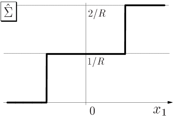 |
| (a) energy density | (b) | (c) |
We can also express topological charges in terms of and its derivative . The BPS bound (2.19) is now rewritten as
| (3.10) |
where we have used and . In the context of the domain wall, the quantity provides the sum of the charges (masses) of the domain walls [14]. Interestingly, the energy of the BPS configuration can be determined only from , namely the zero mode of the overall gauge field . This is because the topological charge is determined only from the boundary condition and all the massive KK-modes vanish at spatial infinities in the BPS configurations.
We finally discuss the Kähler metric on the moduli space of BPS vortices. The moduli space of the vortices is a Kähler manifold parametrized by the moduli parameters . The Kähler metric of the moduli space is directly calculated from the solution of the master equation as follows [6] (see also [23, 18])
| (3.11) | |||||
| (3.12) |
where are derivatives with respect to the moduli parameters and is the length scale of the vortex core. Note that the matrix-valued function depends on the parameters and only through .
For concreteness, let us consider -vortex configurations in the Abelian-Higgs model (). In this case the -dimensional moduli space is parameterized by the positions of vortices . For well-separated vortices , the asymptotic metric is obtained by taking the limit . In the small vortex limit the Kähler metric becomes
| (3.13) |
Therefore the Kähler potential , which determines the metric by a relation , can be written by
| (3.14) |
where and is a holomorphic function which is required to make the Kähler potential finite. This is a one-dimensional “tropical polynomial” that we will extend to the two-dimensional case in the next section. Since the asymptotic forms of the function are given by
a possible choice of the function is
| (3.18) |

Then the asymptotic Kähler potential can be evaluated as the area of the shaded region in Fig. 2, which is given by
| (3.19) |
Using this Kähler potential, the Kähler metric is given by . So the effective Lagrangian which describes the dynamics of well-separated vortices becomes
| (3.20) |
This shows that the well-separated vortices behave as undistinguished free particles with the mass .
In the next section, we move on to the case of vortex on . Although the story is more complicated and general, we will encounter similar structures to those described in this section.
4 Webs of Vortex Sheets on
4.1 Vortex Sheets and Amoeba
Let us consider the vortex-instanton system on . As before, we will use and as real and complex coordinates of , respectively. The coordinates of are identified with periods , namely . In this case, the determinant of the moduli matrix , which defines the vortex sheets, is written in the form of the Fourier series
| (4.1) |
If we define new cylindrical coordinates on by , is now written by a Laurent polynomial
| (4.2) |
The positions of the vortices are described by zeros of similarly to those on in the previous section, but the vortices form a two-dimensional sheet (surface) in in the present case.
We define the “Newton polytope” of a Laurent polynomial by
| (4.3) |
Conversely, is called the Newton polynomial of , when its Newton polytope is convex. In the discussion of domain wall webs, the Newton polytope was called the “grid diagram” [26]–[30]. When we say “Newton polynomial”, the coefficients in (4.2) are arbitrary parameters. Namely, are regarded as moduli parameters of the vortices.
Analogous to the case of the vortices on the cylinder discussed in the the previous section, a web of vortices on is now dimensionally reduced to a web of domain walls on [26]–[30]. In order to see the connection better, we define “amoeba” of by1414 14 Amoeba can be defined for with arbitrary integer , but we only use the case of .
| (4.4) |
Note here that and . This is a projection of the shape of vortex sheet onto two non-compact directions. See Fig. 3 for an example of amoeba.
 |
 | |
| (a) Newton polytope | (b) amoeba |
From this example, we can see that the amoeba has several asymptotic regions extending to infinity, which are called “tenticles” in literature. In physics terms, each of these tenticles represents a semi-infinite cylinder of the vortex, and, for generic coefficients, corresponds to the normals to the Newton polytope (see Fig. 3).1515 15 When moduli parameters are chosen to be special value, several tenticles of amoeba can merge into one. In this case, the multiplicity of the spires is considered to be greater than one. We also have (again, for generic values of moduli) holes for each internal lattice point of the Newton polytope. We learn from these facts that amoeba is a projection of generic webs of the vortices.
The notion of amoeba dates back to [44]. It was originally studied in the context of monodromy of the so-called GKZ-hypergeometric (originally called -hypegeometric) functions. It is also intimately connected with real algebraic geometry (Hilbert’s 16th problem). Furthermore, it plays an important role in the discussion of the tropical geometry, as we will see. What we have found is that amoeba also appears quite naturally in the discussion of the webs of the vortices. See also the work [38], which discusses amoeba in the context of instanton counting.
To see the relation between the webs of the vortex sheets and the webs of the domain walls, it is convenient (just as in the previous section) to define by
| (4.5) |
and similarly for by interchanging the subscript 1 with 2. These adjoint scalar fields on are interpreted as the zero modes of the gauge fields in the Kaluza-Klein decomposition and exhibit the two-dimensional kink profiles. The trace of these adjoint scalar fields can be simply written as
| (4.6) | |||||
where we have used Eq. (2.10) and . The matrix-valued function is simplified in the strong gauge coupling limit to (recall master equation (2.14))
| (4.7) |
Although the vortex sheet becomes thin and singular in the strong coupling limit, the matrix still has important physical informations on vortices and instantons. The traces of the adjoint scalar fields Eq. (4.6) in the strong coupling limit are given by
| (4.8) |
where is nothing but the “Ronkin function” [45] in two dimensions
| (4.9) | |||||
defined from the Laurent polynomial .
The Ronkin function has several interesting properties. First of all, it is convex [45]. Second, the derivatives of the Ronkin function, and , take constant values in each complement of the amoeba,1616 16 In [46] and many other literature, these constant values are called the orders of the complement of the amoeba. and those constant values (multiplied by ) are given by the lattice points in the Newton polytope of [46]. More generally, as a function defined on (including points on the amoeba) take values within the Newton polytope of .
4.2 Relation with Tropical Geometry
Now one difference arises from the previous section. In the complex one-dimensional case discussed in the previous section, the Ronkin function is piece-wise linear when we take the thin wall limit . In two-dimensional case, however, the Ronkin function and its derivative are smooth even when the gauge coupling goes to infinity.
We can still consider another limit in which the derivative of the Ronkin function becomes discontinuous. The limit is with fixed
| (4.10) |
This limit corresponds to dimensionally reducing the theory to (2+1)-dimensions, neglecting all KK modes. In this limit, the amoeba degenerates into a set of lines (“spines”), which is called “tropical variety” in the tropical geometry literature. Physically speaking, the vortices reduce to the domain walls by dimensional reduction, and the tropical variety signifies the location of the domain walls. At the same time, the Ronkin function becomes a piece-wise linear function defined by
| (4.11) |
where is a set of the vertices associated with the Newton polytope , and in Eq.(4.10) are constants determined from constants in (4.2). This function coincides with the Ronkin function on the complement of the amoeba (recall is linear on each complement).
If we compare (4.11) with (4.2), we notice that the sum and products in the polynomial are replaced by a maximum function of the linearized functions. The formal reasoning is given as follows. If we define , , , and , then we find
| (4.12) |
in the limit. Hence in the tropical limit, the ring is replaced by an idempotent semiring1717 17 A semiring is an algebraic structure similar to a ring, but without the requirement that each element must have an additive inverse. , with a tropical addition and a tropical multiplication given by
| (4.13) |
respectively. The semiring is sometimes called the tropical semiring or the max-plus algebra.
The operation replacing the addition and multiplication with the tropical addition and tropical multiplication is also called dequantization or ultradiscretization. It appears in a discretization of integrable soliton equations such as KdV, Toda and KP hierarchies and also in cellular automata. These integrable soliton systems seem to be completely different from the vortex-instanton system we are considering, but it is interesting that the same structure plays important roles in many integrable systems.
We have mentioned about the tropical limit and tropical semiring, but then what is the corresponding geometry? In usual algebraic geometry, we consider geometry corresponding to commutative ring. In contrast, the geometry corresponding to tropical semiring is called tropical (algebraic) geometry.1818 18 According to [47], the name “tropical” was coined by a French mathematician Jean-Eric Pin [48], in honor of their Brazilian colleague Imere Simon [49]. We can formulate and prove “tropical analogue” of many theorems in usual algebraic geometry, such as the Riemann-Roch theorem and the Bezout’s theorem. Although the study of idempotent semirings in applied mathematics (such as control theory and optimization) has a long history [50], the study of corresponding geometry is relatively new and it is still an active area of research (see [51, 47, 52]). The tropical geometry has now diverse applications, ranging from string networks [53], enumeration of curves [54], mirror symmetry [55] and even computational biology [56].
We can consider a tropical version of algebraic variety, namely tropical variety. In the literature, it is often defined as a non-Archimedian amoeba, but for our applications, it suffices to define it as the set of points where the piece-wise linear function (“tropical polynomial”) is not differentiable. This is nothing but the skeleton (spine) of the amoeba in the limit , and its physical meaning is the position of the domain walls, namely the position of the step-wise kinks appearing in the profiles of . An example of the tropical varieties are shown in Fig. 4. As shown there, tropical varieties (in the situation we want to consider) are obtained from triangulation of the Newton polytope ([51], Proposition 3.5). In this sense, this is similar to the so-called -web or web diagram in [57]. We will make more comments on this analogy in the last section devoted to the discussion.
|
 | |
| (a) amoeba | (b) tropical variety |
Example
Let us here give a simple and concrete example for later discussions. An example of the Newton polytope is given in Fig. 5 (a) and we set for simplicity in the following. Then the corresponding Newton polynomial is given by
| (4.14) |
and its amoeba and corresponding variety is shown in Fig. 5.
 |
 |
 |
| (a) Newton polytope | (b) amoeba | (c) tropical variety |
The derivatives Tr of the Ronkin function associated with are computed to be
and their plots are given in Fig. 7. Note that takes a constant value at each complement of amoeba, as expected.
 |
 | |
| (a) Ronkin function | (b) gradient of Ronkin function |
 |
 | |
4.3 Topological Charges
We now move on to discussion of the topological charges given in (2.4) and (2.5). For a given Laurent polynomial , these topological charges are evaluated as follows. First let us consider the vortex charge. Since the topological charges are independent of the gauge coupling constant , we can take the strong gauge coupling limit . In the strong gauge coupling limit, the magnetic flux of the overall can be written as
| (4.23) |
where . By using the Poincaré-Lelong formula1919 19 This formula is the generalization of the formula with .
| (4.24) |
we can show that the vortex charge can be evaluated as
| (4.25) |
From this computation, it is clear that the vortex charge is distributed on the surface of the vortex sheets .
We also see that the vortex charge is uniformly distributed along all , and the total vortex charge is given by the area of the vortex sheets multiplied by the tension . It is interesting to note that the same formula has appeared in mathematics literature ([58], Theorem 6 and [59]).
We can also give another expression for the vortex charge, using the Ronkin function . In the tropical limit , the vortex charge is given by
| (4.26) |
where . Namely, vortex charge is given by an integration of a Laplacian of the Ronkin function. If we take the limit , the amoeba becomes the tropical variety which can be interpreted as the web diagram of the domain walls. The tension of each wall can be calculated as follows. Since the integrand of Eq. (4.26) becomes in the small radius limit , the tension of the domain wall is computed by integrating the Laplacian of the piece-wise linear function along the line perpendicular to the wall. If the wall is located along the line , then the tension is given by
| (4.27) |
Next let us consider the intersection charge (2.8). By taking the strong gauge coupling limit, the intersection charge density becomes a complex Monge-Ampère measure on associated with a plurisubharmonic2020 20 Monge-Ampère measure is defined for arbitrary plurisubharmonic function. Here it suffices to know that is plurisubharmonic for arbitrary holomorphic function . function , which is a higher dimensional generalization of the Laplace operator (see [60, 61] for discussion on the complex Monge-Ampère measure):
| (4.28) | |||||
Then the intersection charge is evaluated again by using Poincaré-Lelong formula,
| (4.29) |
but this naive evaluation is unfortunately divergent. The divergence comes from the fact that the strong gauge coupling limit in the master equation (2.14) is ill-defined when , since there appears in the master equation. In principle, if we can solve master equation for finite gauge coupling, we could safely obtain a correct value of the intersection charge, but that would be difficult in practice. Instead, we propose to regularize the divergence as follows.
Let and be distinguished Laurent polynomials associated with the same Newton polytope of , and replace two ’s in (4.29) by and , respectively. For generic Laurent polynomials and , the intersection points of the zero sets of and are discrete points. Then we obtain
| (4.30) |
where the surfaces are defined by and the number of intersection points are denoted as .
Thanks to Bernstein’s theorem [63],2121 21 This theorem is a generalization of the well-known Bezout’s theorem. See [62] for leisurely introduction to Bernstein’s theorem. is independent of the choice of the Laurent polynomials as long as and are generic, and is given by . We thus find that the intersection charge is evaluated to be equal to the area of the Newton polygon:
| (4.31) |
The meaning of this regularization is now clear. The original expression (4.29) is divergent essentially because it is a self-intersection number. We propose to regularize this by infinitesimally changing , but with fixed boundary conditions at infinity.2222 22 The condition that and are Newton polynomial of the convex polytope is important. Otherwise the answer depends on the choice of and . For example, if we take , , then for all . If we take instead , then . And for (in a neighborhood of ), . All these functions converge to the same in the limit, but gives a different answer. We thank Alexander Rashkovski for providing us with this example.
Instead of invoking Bernstein’s theorem, we can take more down-to-earth approach and the calculation goes as follows. This derivation is not independent from the previous argument and moreover not rigorous, but it has an advantage of clarifying the relation with the Ronkin function and real Monge-Ampère measure.
First, it is reasonable to expect2323 23 Essentialy, we are again using Bernstein’s theorem here for the rigorous argument. that the intersection number does not change under replacements and , as far as and are sufficiently generic:
| (4.32) |
where
| (4.33) | |||||
| (4.34) |
Certainly the intersection number (4.32) might change if and are non-generic, but those special values do not contribute when we integrate over all and . The same applies to and . Therefore the intersection charge can be written as
| (4.35) | |||||
where
| (4.36) |
is known as a real Monge-Ampère measure,2424 24 More precisely, when , this is called a real mixed Monge-Ampère measure. which is a real analogue of the complex Monge-Ampère measure we explained previously. Note that this is well-defined since is convex, as discussed previously. If we set , then
| (4.37) | |||||
| (4.38) | |||||
| (4.39) |
In the final line we used the fact that takes values in the Newton polytope , as explained previously. Interestingly, this result, that the total integral (or “mass” in the standard mathematics literature) of the real Monge-Ampère measure is given by , has appeared previously in the mathematics literature ([58] Theorem 4).
From the above calculation, we have shown that the evaluation of the complex Monge-Ampère measure reduces to the evaluation of the real Monge-Ampère measure. Since the Ronkin function is described by the zero mode in the KK decomposition, we learn from this fact that contributions from KK modes, although present, are canceled out in the final expression. This is just the same as in the discussion in Sec. 2: topological charge is determined only from the boundary condition and all KK modes vanish at spatial infinity.
We can provide one more different explanation of the formula , which is much easier to understand (although strictly speaking, this is also just a restatement of the previous explanation). Taking the limit , the intersection charge is given by the half of the intersection number of the tropical varieties of and , and it is easy to see that the number is given by (see Fig. 8 for example). In tropical geometry, this statement is known as the tropical Bernstein theorem ([64] Theorem 9.5).

Although the computation here applies only to limit, we expect that the intersection charge is still given by the same formula for finite as well, since the intersection charge is quantized and does not change continuously depending on . For the same reason, although all the arguments so far are in the strong gauge coupling limit , we expect the same formula is kept in the finite gauge coupling as well.
So far, we have concentrated on the case of called local theory. We expect that a similar formula holds even for , which is often called semi-local theory. For , we can actually show this rigorously.2525 25 We thank Alexander Rashkovskii for providing us with the following proof. In the strong gauge coupling limit the solution of the master equation Eq. (2.14) for is given by
| (4.40) |
In this case, needs no regularization. We use two representations of the current (intersection charge density) for . One is King’s formula (a.k.a. the vector Poincaré, or the Poincaré-Martinelly formula [61, 65])
| (4.41) |
and another is
| (4.42) |
which follows from Poincaré-Lelong formula applied to on . We thus have
| (4.43) | |||||
| (4.44) |
where in the last line we have again used Bernstein’s theorem, and is a mixed volume defined by
| (4.45) |
and the sum (Minkowski sum) is defined by
| (4.46) |
For general and , the solution of the master equation Eq. (2.14) in the strong coupling limit is given by
| (4.47) | |||
| (4.48) |
Therefore the intersection charge can be evaluated by integrating with being an -dimensional vector. Unfortunately, we have no mathematical estimate for , and only the upper bound [66] for the integral of the complex Monge-Ampère measure in (not ) is known. We conjecture that the result holds in this more general case in the same manner.2626 26 At least, we can prove that intersection charge is quantized. We thank Alexander Rashkovskii for providing us with this argument. The argument goes as follows. Let be a -dimensional vector . For a two-dimensional subspace of the -dimensional complex space , let be , where is the -matrix of orthonormal basis of . Then by [61, 67], Monge-Ampère measure is represented as where is the Haar measure on the complex Grassmannian . Note is well-defined for all except for an algebraic subset of which is zero measure. Since has exactly two components, it follows from the discussion of case that is given by the intersection number of and , which is an integer. This means is an integer-valued continuous function. We have now proved that the value of is quantized.
This concludes our discussion of the topological charges. Our discussion mainly concentrates on the case . As we have seen, however, even for case, the overall part represented by is still described by the language of the amoeba and tropical geometry. At the same time, we should not think that is the whole story. Out of all the topological charges (2.5), (2.8) and (2.9), the instanton number
| (4.49) |
vanishes in theory and appears only in non-Abelian theory. We will discuss this in the next section, but before that let us discuss metric of moduli space for the web of vortices.
4.4 Metric on Moduli Space
In this section, we discuss the metric of the moduli space. The metric of the moduli space is given by a formula similar to the one-dimensional case, Eq. (3.11) and Eq. (3.12),
| (4.50) |
This is a new result which is valid for arbitrary values of and .
Here we focus on the case in which all the moduli parameters are contained in the Laurent polynomial. Let us consider a Newton polytope associated with a Laurent polynomial . Let and be sets of external and internal vertices of , respectively. The coefficients of the Laurent polynomial are identified with the moduli parameters and there exist zero modes corresponding to these moduli parameters.
| (4.51) |
The coefficients determine the positions of the external legs and the size of the loops of the vortex web, while the coefficients determine only the size of the loops of the vortex web. Since the zero modes associated to the motion of the external legs are non-normalizable, we cannot define the metric for these zero modes and we must fix the moduli parameters .
First let us consider the case where the loop sizes and the radii of the torus are much larger than the width of the vortex sheets . In this case we can evaluate the leading terms in the Kähler metric by taking the thin vortex sheet limit
| (4.52) |
From Eq.(4.9) we obtain the Kähler potential in the thin vortex sheet limit as
| (4.53) |
Here is a holomorphic function with respect to and it should be chosen to make the Kähler potential finite. A possible choice of the function is
| (4.54) | |||||
| (4.55) |
Therefore the Kähler potential can be evaluated by integrating the Ronkin functions.
Next let us consider the case where the loop sizes are much larger than the radius of torus . In this case the leading terms in the Kähler potential can be evaluated by taking the small radius limit of Eq. (4.53). Since in the limit , the leading term in the Kähler potential is given by
| (4.56) | |||||
where and are piece-wise linear functions defined by
| (4.57) | |||||
| (4.58) |
with .
Let us consider the simplest example of one-loop configuration associated with the Laurent polynomial
| (4.59) |
 |
 |
|
| (a) Newton polytope | (b) web diagram (tropical variety) |
.
In this case the vertices of the Newton polytope are
| (4.60) | |||||
| (4.61) | |||||
| (4.62) |
There exists only one normalizable moduli parameter for which we can define the metric. This moduli parameter is related to the size of the loop in Fig. 9-(b), which is proportional to . The non-normalizable moduli have already been fixed to 1 in Eq. (4.59). The Laurent polynomial defined in Eq. (4.55) is given by
| (4.63) |
The piece-wise linear functions and defined in Eq. (4.58) are now given by
| (4.64) |
By integrating Eq. (4.56), we obtain the asymptotic Kähler potential as the volume of a tetrahedron in Fig. 10, which is given by
| (4.65) |

Differentiating the Kähler potential Eq. (4.65), we obtain the metric of the moduli space and then the effective Lagrangian
| (4.66) |
Here is the phase of the moduli parameter . This asymptotic Lagrangian can be interpreted as the kinetic energy associated with the motion of the three vortices composing the loop. Since they can be interpreted as walls with tension and , two of three vortices have the mass and the other vortex has the mass . If the moduli parameter varies with velocity , the vortices move in the -plane with velocities and . Then the total kinetic energy associated with the motion of the vortices is .
5 Instantons inside Non-Abelian Vortex Webs
In this section, we discuss the instanton number as promised in the previous section. We consider the case of gauge theory with scalar fields as the simplest model which admits the BPS configuration with . The generalization to the gauge group should be straightforward.
5.1 Instanton Number on a Planar Vortex Plane: a Review
Let us first review the 1/2 BPS vortex moduli space. The vacuum of gauge theory with scalar fields breaks the color and flavor symmetry into color-flavor locked symmetry . The 1/2 BPS single vortex in this theory further breaks into . Therefore there appear Nambu-Goldstone modes of the complex projective space localized around the vortex [2, 3]. The orientation moduli form a part of the moduli space.
The moduli matrix for the vortex at with an orientational moduli parameter is given by [5]
where represents the -equivalence relation. These two moduli matrices provide two patches and of [5]. For this moduli matrix, the solution of the master equation is given by
where is a solution of the master equation in the case of the Abelian-Higgs model (), such that
| (5.9) |
Therefore once the vortex solution of the Abelian-Higgs model is given, one can construct the whole solution of the non-Abelian model.
Next let us discuss the 1/4 BPS configuration of instantons and vortices on . The 1/2 BPS vortex plays the role of a host soliton in the 1/4 BPS vortex-instanton configuration. It has an internal degree of freedom parametrized by an orientational moduli parameter , which is interpreted as an inhomogeneous coordinate of as denoted above. The instantons inside the vortex can be constructed as lumps in the vortex effective theory which is the sigma model [22, 23]. By using the moduli matrix (5.1) for 1/2 BPS single vortex, we can construct the moduli matrix for some 1/4 BPS configurations as follows. The moduli matrix for the 1/4 BPS vortex-instanton configuration is obtained by promoting the orientational moduli to a holomorphic function of the other holomorphic coordinate [23]
where the moduli parameter denotes the position of the -th instanton and determines the overall size of the instantons on the vortex sheet defined by . This function is regarded as a holomorphic map from the vortex sheet to .
In order to compute the instanton number, we require the information upon the solution of the master equation for the moduli matrix Eq. (5.1). Since the topological charges are determined only from the boundary condition, it can be calculated from the asymptotic behavior of the solution which is obtained by the following procedure. Solving the BPS equation in the 2+1-dimensional effective theory on the vortex worldvolume, we obtain the lump solution corresponding to the instanton inside the vortex sheet. Substituting back the solution of the effective theory into the 1/2 BPS vortex solution Eq. (5.1), we find
Although this is not an exact solution of the master equation since is not a constant, we can see that this matrix possesses the correct asymptotic behavior at spatial infinity by substituting into the master equation. Therefore the topological charge, which is determined by behavior of the fields at spatial infinity, can be evaluated from this matrix . Inserting into Eq. (2.4), we obtain
| (5.16) |
Therefore the instanton charge is measured by the degree of the function , namely the degree of the holomorphic map from the vortex sheet to .
5.2 Instanton Number on Non-Abelian Vortex Webs
As we have seen in the example above, the instantons can exist on the planar vortex sheets. Now we work out more general 1/4 BPS configurations explicitly. The planar host vortex sheet can be extended to a general web of the vortex sheets characterized by as discussed in the previous sections. We therefore replace the lower-right component in the moduli matrix (5.1) by . Moreover the holomorphic function in (5.1) is also replaced with a function of two holomorphic coordinates and . The moduli matrix for such 1/4 BPS configuration of the instantons and vortex sheets on thus becomes
where and are Laurent polynomials
| (5.20) |
Although Eq. (5.2) is not the most general form of the moduli matrix for the 1/4 BPS configurations, we treat this simple form of the moduli matrix for essential explanation. The coefficients of the Laurent polynomials and are the moduli parameters which give the location of vortex sheets, and the positions and sizes of the instantons, respectively.
For the moduli matrix Eq. (5.2), the instanton charge in Eq. (2.4) is computed as follows. Since the topological charge should not change under continuous deformations, we can take a strong coupling limit in which the solution of the master equation approaches to
However a direct calculation does not work since the vortex sheets become singular in this limit. To avoid the calculation involving the singular vortex sheets, we perform another deformation of the configuration. Similarly to the case of the planar vortex sheet, let be a matrix given by
where is a solution to the following equation
| (5.27) |
Although the matrix is not a solution of the master equation unless the holomorphic function is constant everywhere, this matrix has the correct topological information about the configuration similarly to the planar case. For this matrix , we can show that
| (5.28) | |||||
If we take the strong gauge coupling limit in Eq. (5.27), then approaches to . Therefore we obtain the instanton charge in Eq. (2.4) as
| (5.29) |
where the first term gives the instanton number in Eq. (2.9) and the second term gives the intersection charge in Eq. (2.8) which has been computed in Sec. 4.3. The instanton number is rewritten by using the Poincaré-Lelong formula
| (5.30) |
where denotes the zero locus of corresponding to the vortex sheets. Therefore the instanton number is given by the degree of the map .
To see a distribution of the topological charge density, we take two limits of the parameters: one is a small instanton limit and the other is a small radius limit . The small instanton limit is realized by taking the limit with fixed ratios . Then the two form has a delta function-like support on the zeros of . From this fact we find that in the small instanton limit the instantons are localized at common zeros of and , and that the vortex sheets are located at . We also find that instantons are localized at the positions of lumps from the viewpoint of effective theory on the vortex sheets.
 |
 |
 |
| (a) | (b) | (c) |
 |
 |
| (d) | (e) |
Next, let us consider the small radius limit . In this limit, the function becomes
| (5.31) |
where and for are fixed in the limit. Then the instanton number takes the form
| (5.32) | |||||
Therefore the instanton number density is localized at the intersection of the tropical variety of the Laurent polynomial and the lines on which the piece-wise linear function is not differentiable. When the instanton number density is localized at the intersection of the lines and , the instanton number is given by
Fig. 11 shows examples of the instanton number density on for and . Varying the moduli parameters, the instantons localized at the intersection move along the tropical variety of . For each intersection in Fig. 11(a)-(d) the instanton number is . In Fig. 11(e) instanton, which can be interpreted as the coincident instantons, is localized at the intersection of the lines and .
So far we have treated the specific configuration of the non-Abelian vortex sheets and instantons on and the specific gauge group . For more general cases, the computation of the instanton number seems to be complicated and difficult, but the essence should be similar to the above calculations.
6 Conclusion and Discussion
In this paper, we have investigated generic intersections (or webs) of vortices with instantons inside, which is a 1/4 BPS state in the Higgs phase of (the bosonic part of ) five-dimensional supersymmetric gauge theory on with Higgs scalars in the fundamental representation. We have found that this vortex-instanton system can be beautifully and naturally understood in the mathematical framework of the amoeba and tropical geometry, and have proposed a dictionary relating the solitons and gauge theory to the amoeba and tropical geometry (summarized in Table 1).
| soliton/gauge theory | amoeba/tropical geometry |
|---|---|
| moduli matrix | Newton Polynomial |
| projection of vortex sheet | amoeba |
| tropical limit | |
| position of step-wise kinks | tropical variety |
| Wilson loop | derivative of Ronkin function: , (4.9) |
| intersection charge | (total mass of) complex Monge-Ampère measure |
| vortex charge density | Laplacian of Ronkin function: (4.26) |
In this discussion, the moduli matrix formalism has played crucial roles. The solutions to 1/4 BPS equations are parametrized by a holomorphic function (Laurent polynomial) of two complex parameters of . This Laurent polynomial can also be considered as a Newton polynomial of some convex polytope , namely the grid diagram. In the strong gauge coupling limit, the position of vortices is exactly given by the zero of , while the projection of the shape of vortex sheet is the amoeba of . Moreover, we can relate Wilson loops in , or the zero modes of gauge fields in Kaluza-Klein decomposition, to the derivatives of the Ronkin function , which is a convex function and is defined from Newton polynomial .
The relation with the tropical limit and tropical geometry has also been discussed. In the discussion of solitons, it is natural to consider dimensional reduction of the theory in order to obtain BPS solitons in lower-dimensional field theories. This limit is known in the mathematical literature as the tropical limit. In this limit, the shape of amoeba degenerates into a tropical variety, which is nothing but the so-called -web of the grid diagram. We have shown that tropical geometry provides simple and elegant method to understand not only the dimensionally reduced theory but also the original vortex-instanton system on .
We have also discussed the topological charges, which are divided into three types. They are the vortex charge , the intersection charge (negative contribution of the instanton charge) and the instanton number . First, the vortex charge is uniformly distributed along vortex sheet det, and its density is given by the Laplacian of the Ronkin function in the tropical limit. Its total charge is the area of the vortex sheet multiplied by . Second, in the strong gauge coupling limit the intersection charge density is given by the complex Monge-Ampère measure of a plurisubharmonic function , and total intersection charge is given by the area of the grid diagram with a suitable regularization. Third, the instanton number appears only in the non-Abelian case, and we have discussed the case of as an example. Our discussion simplifies in two limits. In the small instanton limit, instantons are localized at intersections of and another Laurent polynomial , which parametrizes an orientational moduli . In the small radius limit, the instanton number density is localized at the intersection of the tropical varieties corresponding to and . We have also obtained the general form of the Kähler potential and the asymptotic metric of the moduli space of a vortex loop as a byproduct of the discussions above. In the tropical limit, the Kähler potential is given by the volume of a convex polytope, and the effective Lagrangian can be interpreted as the kinetic energy associated with the motion of vortices composing the loop.
In our discussion, we mainly focused on the case of Abelian-Higgs model (), but as far as the overall part is concerned the story is exactly the same in non-Abelian case. We also obtained new results by going to non-Abelian gauge group, such as the instanton number. This seems to suggest a non-Abelian generalization of the amoeba and tropical geometry.
Despite such impressive success, there are still many points which need further exploration.
First, in this paper, we have found one-to-one correspondence between the amoeba/tropical geometry and solitons in Abelian gauge theory. However the configuration of instantons inside non-Abelian vortex-webs in non-Abelian gauge theory discussed in Sec. 5 does not correspond to the amoeba and tropical geometry so far. This configuration suggests non-Abelian generalization of amoeba and tropical geometry. Furthermore the non-Abelian vortices have been recently extended to the case of gauge group with arbitrary simple group [12]. This is the case of complex one dimension. It should be extendible to the case of complex two dimensions such as . That may suggest further generalization of the amoeba and tropical geometry associated to arbitrary group, which contains the usual one as a special case of gauge group.2727 27 In fact, the motto of tropical geometry is to extend usual algebraic geometry by replacing commutative ring with a commutative semiring. Another generalization is to replace a commutative ring with a non-commutative ring, which is non-commutative geometry. Perhaps our discussion of non-Abelian vortices suggests further generalization by combining above two, which should be called “non-commutative/non-Abelian tropical geometry”.
Second, let us pursue a possibility to generalize the space where the amoeba lives. In this paper we have considered the amoeba on . This is because the maximal space-time dimension of supersymmetric gauge theory with eight supercharges is . Since space-dimension is odd we have studied four dimensional case . If we abandon implementing supersymmetry, we can extend the bosonic Lagrangian (2.1) to space dimensions higher than , and study higher co-dimensional composite solitons of the vortices and instantons extending to various directions. In fact the generalized vortex equations on arbitrary Kähler manifold of arbitrary dimensions were obtained in (bosonic) Yang-Mills-Higgs theory [39]. Therefore we expect those equations give further correspondence of the amoeba and gauge theory on or on general Kähler manifolds.
The third topic is the relation with dimer model [68, 69]. Dimers do not appear directly in our discussion, but it is known that dimer model is intimately connected with the amoeba and tropical geometry. For example, the Ronkin function as defined in (4.9) coincides with the thermodynamic limit of partition function of a dimer model. Moreover, a spectral curve of the dimer model is known [68] to parametrize Harnack curve, whose amoeba has good properties. The dimers also appear in discussion of the brane tilings [70, 71] and four-dimensional superconformal quiver gauge theories. The brane tilings now have an interpretation as configuration of D5-branes and NS5-brane [72], whose brane configuration is shown in Table 2,
| 0 | 1 | 2 | 3 | 4 | 5 | 6 | 7 | 8 | 9 | |
|---|---|---|---|---|---|---|---|---|---|---|
| D5 | ||||||||||
| NS5 | (2-dim surface) | |||||||||
wherein is a two-dimensional surface in 4567-directions. In the weak gauge coupling limit, this is the zero locus of a Newton polynomial with respect to two complex variables in . Hence the mathematical structure of the NS5-brane is exactly the same as that of the vortex sheets we have considered in this paper. The toric diagram and the grid diagram are identical, and the meaning of the tropical limit and tropical variety also coincides. Of course, we should keep in mind that there exists important differences between the soliton systems in this paper and the brane tilings. First, in this paper we have assumed systems with eight supercharges, but in brane tiling, we have only four supercharges. Related to this fact is that we do not have analogue of D5-brane in the soliton side, and have the instanton charge instead. Still, we might obtain something new from this analogy. For example, in the discussion of brane tilings, the projection of on to directions, which is called alga or coamoeba, plays crucial roles [37, 73]. It would be interesting to see whether coamoeba has any significance in our setup. Perhaps we can understand these points better if we can find a D-brane realization of the vortex-instanton system. For this direction, the work on D-brane configuration of vortices on cylinder [7, 11], its T-dual to the D-brane configuration of the domain walls[15, 16], and the D-brane configurations of the domain wall webs [28] should be a useful guideline.
The amoeba and tropical geometry also appear in the computation of the topological string amplitude and the instanton counting in 4d and 5d supersymmetric gauge theories. Their perturbative dynamics are ruled by asymptotic behavior of the (plane) partitions where the amoeba and the Ronkin function appear. It is also pointed out that the Kähler structure behind the theories is closely related with the volume of the convex cone of the Ronkin function similarly to our discussion on the Kähler potential. These relations suggest that the intersecting soliton system also admits an interpretation of the microscopic partitions (dimers) and that the Kähler geometry of the moduli space of the solitons is determined by a suitable asymptotic limit of the microscopic interpretation.
Finally, statistical partition functions of the vortices on a cylinder were studied by using D-brane configurations [11]. There the integration over the moduli space of vortices is drastically simplified in the T-dual picture: vortices are mapped to domain walls and the integration reduces to a problem of rods. The limit of parameters employed in [11] is a little different from that in this paper. There the limit was taken with fixed wall width , while in this paper we have taken the strong coupling limit first and then the small radius limit . This is nothing but the non-linear sigma model version of the limit in [11]. In the case of , the gauged linear sigma model reduces to the non-linear sigma model and the vortex solution reduces to the lump solution [10]. The lump solution on the cylinder can be mapped to kinks on one-dimensional space. The small radius limit , which corresponds to dequantization (ultradiscretization) limit , enable us to identify the kinks with free particles in one-dimensional space as in Sec. 3. The partition function of the free particles gives the exact volume of the moduli space of the sigma-model lumps, namely the partition function for a multi-lump system. This fact and the result of [11] suggest that the procedure of the dequantization is powerful enough to give the exact partition function of the solitons in non-linear sigma model and variant of it makes the computation of the partition function very simple even in the case of finite gauge couplings. This should be extendible to the vortex webs discussed in this paper, to obtain a partition function of the instanton-vortex system. We expect that it will be reduced to the Nekrasov’s partition function in the limit of where the vortices disappear while the instantons still remain. The integration over the moduli space of the instanton-vortex system may provide a systematic method to compute the symplectic Gromov-Witten invariant, which is a combination of the Donaldson invariant and the Gromov-Witten invariant [74].
Acknowledgements
We are grateful to Minoru Eto, Takayuki Nagashima and Keisuke Ohashi for collaboration in early stages of this project. We would like to thank the Yukawa Institute for Theoretical Physics at Kyoto University, where this work was initiated during the workshop YITP-W-06-16 on “Foundamental Problems and Applications of Quantum Field Theory”. M.N. and K.O. are supported in part by Grant-in-Aid for Scientific Research (No. 20740141 and No.19740120, respectively) from the Ministry of Education, Culture, Sports, Science and Technology. T. F. and M.Y. are supported by the JSPS Research Fellowships for Young Scientists. This work is supported in part by Grant-in-Aid for Scientific Research from the Ministry of Education, Culture, Sports, Science and Technology, Japan No.17540237 and No.18204024 (N.S.). M.Y. would like to thank Yosuke Imamura for discussions, Alexander Rashkovskii for kind correspondence, and Yukawa Institute for Theoretical Physics for hospitality during the final stages of this work.
References
- [1] A. A. Abrikosov, Sov. Phys. JETP 5, 1174 (1957) [Zh. Eksp. Teor. Fiz. 32, 1442 (1957)]; H. B. Nielsen and P. Olesen, Nucl. Phys. B 61, 45 (1973).
- [2] A. Hanany and D. Tong, JHEP 0307, 037 (2003) [arXiv:hep-th/0306150].
- [3] R. Auzzi, S. Bolognesi, J. Evslin, K. Konishi and A. Yung, Nucl. Phys. B 673, 187 (2003) [arXiv:hep-th/0307287].
- [4] R. Auzzi, S. Bolognesi, J. Evslin and K. Konishi, Nucl. Phys. B 686, 119 (2004) [arXiv:hep-th/0312233]; M. Eto, M. Nitta and N. Sakai, Nucl. Phys. B 701, 247 (2004) [arXiv:hep-th/0405161]; V. Markov, A. Marshakov and A. Yung, Nucl. Phys. B 709, 267 (2005) [arXiv:hep-th/0408235]; A. Gorsky, M. Shifman and A. Yung, Phys. Rev. D 71, 045010 (2005) [arXiv:hep-th/0412082]; R. Auzzi, M. Shifman and A. Yung, Phys. Rev. D 73, 105012 (2006) [Erratum-ibid. D 76, 109901 (2007)] [arXiv:hep-th/0511150]; M. Shifman and A. Yung, Phys. Rev. D 73, 125012 (2006) [arXiv:hep-th/0603134]; T. Inami, S. Minakami and M. Nitta, Nucl. Phys. B 752, 391 (2006) [arXiv:hep-th/0605064]; L. G. Aldrovandi, Phys. Rev. D 76, 085015 (2007) [arXiv:0706.0446 [hep-th]]; A. D. Popov, “Integrability of Vortex Equations on Riemann Surfaces,” arXiv:0712.1756 [hep-th]; “Non-Abelian Vortices on Riemann Surfaces: an Integrable Case,” arXiv:0801.0808 [hep-th].
- [5] M. Eto, Y. Isozumi, M. Nitta, K. Ohashi and N. Sakai, Phys. Rev. Lett. 96, 161601 (2006) [arXiv:hep-th/0511088]; M. Eto, K. Konishi, G. Marmorini, M. Nitta, K. Ohashi, W. Vinci and N. Yokoi, Phys. Rev. D 74, 065021 (2006) [arXiv:hep-th/0607070].
- [6] M. Eto, Y. Isozumi, M. Nitta, K. Ohashi and N. Sakai, Phys. Rev. D 73, 125008 (2006) [arXiv:hep-th/0602289].
- [7] M. Eto, T. Fujimori, Y. Isozumi, M. Nitta, K. Ohashi, K. Ohta and N. Sakai, Phys. Rev. D 73, 085008 (2006) [arXiv:hep-th/0601181].
- [8] M. Eto, K. Hashimoto, G. Marmorini, M. Nitta, K. Ohashi and W. Vinci, Phys. Rev. Lett. 98, 091602 (2007) [arXiv:hep-th/0609214].
- [9] M. Eto et al., Nucl. Phys. B 780, 161 (2007) [arXiv:hep-th/0611313].
- [10] M. Eto et al., Phys. Rev. D 76, 105002 (2007) [arXiv:0704.2218 [hep-th]].
- [11] M. Eto, T. Fujimori, M. Nitta, K. Ohashi, K. Ohta and N. Sakai, Nucl. Phys. B 788, 120 (2008) [arXiv:hep-th/0703197].
- [12] M. Eto, T. Fujimori, S. B. Gudnason, K. Konishi, M. Nitta, K. Ohashi and W. Vinci, “Constructing Non-Abelian Vortices with Arbitrary Gauge Groups,” arXiv:0802.1020 [hep-th].
- [13] E. R. C. Abraham and P. K. Townsend, Phys. Lett. B 291, 85 (1992); Phys. Lett. B 295, 225 (1992); J. P. Gauntlett, D. Tong and P. K. Townsend, Phys. Rev. D 64, 025010 (2001) [arXiv:hep-th/0012178]; D. Tong, Phys. Rev. D 66, 025013 (2002) [arXiv:hep-th/0202012]; JHEP 0304, 031 (2003) [arXiv:hep-th/0303151]; K. S. M. Lee, Phys. Rev. D 67, 045009 (2003) [arXiv:hep-th/0211058]; M. Arai, M. Naganuma, M. Nitta, and N. Sakai, Nucl. Phys. B 652, 35 (2003) [arXiv:hep-th/0211103]; “BPS Wall in N=2 SUSY Nonlinear Sigma Model with Eguchi-Hanson Manifold” in Garden of Quanta - In honor of Hiroshi Ezawa, Eds. by J. Arafune et al. (World Scientific Publishing Co. Pte. Ltd. Singapore, 2003) pp 299-325, [arXiv:hep-th/0302028]; M. Arai, E. Ivanov and J. Niederle, Nucl. Phys. B 680, 23 (2004) [arXiv:hep-th/0312037]; Y. Isozumi, K. Ohashi and N. Sakai, JHEP 0311, 061 (2003) [arXiv:hep-th/0310130]; JHEP 0311, 060 (2003) [arXiv:hep-th/0310189]; M. Shifman and A. Yung, Phys. Rev. D 70, 025013 (2004) [arXiv:hep-th/0312257]; N. Sakai and Y. Yang, Commun. Math. Phys. 267, 783 (2006) [arXiv:hep-th/0505136]; A. Hanany and D. Tong, Commun. Math. Phys. 266, 647 (2006) [arXiv:hep-th/0507140]; M. Eto, M. Nitta, K. Ohashi and D. Tong, Phys. Rev. Lett. 95, 252003 (2005) [arXiv:hep-th/0508130].
- [14] Y. Isozumi, M. Nitta, K. Ohashi and N. Sakai, Phys. Rev. Lett. 93, 161601 (2004) [arXiv:hep-th/0404198]; Phys. Rev. D 70, 125014 (2004) [arXiv:hep-th/0405194]; M. Eto, Y. Isozumi, M. Nitta, K. Ohashi, K. Ohta, N. Sakai and Y. Tachikawa, Phys. Rev. D 71, 105009 (2005) [arXiv:hep-th/0503033]; M. Eto, T. Fujimori, M. Nitta, K. Ohashi and N. Sakai, “Domain Walls with Non-Abelian Clouds,” arXiv:0802.3135 [hep-th].
- [15] N. D. Lambert and D. Tong, Nucl. Phys. B 569, 606 (2000) [arXiv:hep-th/9907098].
- [16] M. Eto, Y. Isozumi, M. Nitta, K. Ohashi, K. Ohta and N. Sakai, Phys. Rev. D 71, 125006 (2005) [arXiv:hep-th/0412024].
- [17] D. Tong, “TASI lectures on solitons,” arXiv:hep-th/0509216.
- [18] M. Eto, Y. Isozumi, M. Nitta, K. Ohashi and N. Sakai, J. Phys. A 39, R315 (2006) [arXiv:hep-th/0602170]; “Solitons in supersymmetric gauge theories: Moduli matrix approach,” arXiv:hep-th/0607225.
- [19] M. Shifman and A. Yung, Rev. Mod. Phys. 79, 1139 (2007) [arXiv:hep-th/0703267].
- [20] D. Tong, Phys. Rev. D 69, 065003 (2004) [arXiv:hep-th/0307302].
- [21] M. Shifman and A. Yung, Phys. Rev. D 70, 045004 (2004) [arXiv:hep-th/0403149].
- [22] A. Hanany and D. Tong, JHEP 0404, 066 (2004) [arXiv:hep-th/0403158].
- [23] M. Eto, Y. Isozumi, M. Nitta, K. Ohashi and N. Sakai, Phys. Rev. D 72, 025011 (2005) [arXiv:hep-th/0412048].
- [24] J. P. Gauntlett, R. Portugues, D. Tong and P. K. Townsend, Phys. Rev. D 63, 085002 (2001) [arXiv:hep-th/0008221]; M. Shifman and A. Yung, Phys. Rev. D 67, 125007 (2003) [arXiv:hep-th/0212293].
- [25] Y. Isozumi, M. Nitta, K. Ohashi and N. Sakai, Phys. Rev. D 71, 065018 (2005) [arXiv:hep-th/0405129].
- [26] M. Eto, Y. Isozumi, M. Nitta, K. Ohashi and N. Sakai, Phys. Rev. D 72, 085004 (2005) [arXiv:hep-th/0506135].
- [27] M. Eto, Y. Isozumi, M. Nitta, K. Ohashi and N. Sakai, Phys. Lett. B 632, 384 (2006) [arXiv:hep-th/0508241].
- [28] M. Eto, Y. Isozumi, M. Nitta, K. Ohashi, K. Ohta and N. Sakai, AIP Conf. Proc. 805, 354 (2006) [arXiv:hep-th/0509127].
- [29] M. Eto, T. Fujimori, T. Nagashima, M. Nitta, K. Ohashi and N. Sakai, Phys. Rev. D 75, 045010 (2007) [arXiv:hep-th/0612003].
- [30] M. Eto, T. Fujimori, T. Nagashima, M. Nitta, K. Ohashi and N. Sakai, Phys. Rev. D 76, 125025 (2007) [arXiv:0707.3267 [hep-th]].
- [31] M. Naganuma, M. Nitta and N. Sakai, Grav. Cosmol. 8, 129 (2002) [arXiv:hep-th/0108133]; R. Portugues and P. K. Townsend, JHEP 0204, 039 (2002) [arXiv:hep-th/0203181].
- [32] M. Eto, Y. Isozumi, M. Nitta and K. Ohashi, Nucl. Phys. B 752, 140 (2006) [arXiv:hep-th/0506257].
- [33] K. M. Lee and H. U. Yee, Phys. Rev. D 72, 065023 (2005) [arXiv:hep-th/0506256].
- [34] A. Okounkov, N. Reshetikhin and C. Vafa, “Quantum Calabi-Yau and classical crystals,” arXiv:hep-th/0309208.
- [35] A. Iqbal, N. Nekrasov, A. Okounkov and C. Vafa, “Quantum foam and topological strings,” arXiv:hep-th/0312022.
- [36] N. Nekrasov and A. Okounkov, “Seiberg-Witten theory and random partitions,” arXiv:hep-th/0306238.
- [37] B. Feng, Y. H. He, K. D. Kennaway and C. Vafa, “Dimer models from mirror symmetry and quivering amoebae,” arXiv:hep-th/0511287.
- [38] T. Maeda and T. Nakatsu, Int. J. Mod. Phys. A 22, 937 (2007) [arXiv:hep-th/0601233].
- [39] I. Mundet i Riera, “Yang-Mills-Higgs theory for symplectic fibrations,” arXiv:math.sg/9912150; “A Hitchin-Kobayashi correspondence for Kahler fibrations,” J. Reine Angew. Math. 528 (2000) 41; K. Cieliebak, A. Rita Gaio, D. A. Salamon, “-holomorphic curves, moment maps, and invariants of Hamiltonian group actions,” Internat. Math. Res. Notices (2000) 831 [arXiv:math.SG/9909122].
- [40] A. D. Popov and R. J. Szabo, J. Math. Phys. 47, 012306 (2006) [arXiv:hep-th/0504025]; O. Lechtenfeld, A. D. Popov and R. J. Szabo, JHEP 0609, 054 (2006) [arXiv:hep-th/0603232].
- [41] C. N. Yang, Phys. Rev. Lett. 38, 1377 (1977).
- [42] C. H. Taubes, Commun. Math. Phys. 72, 277 (1980).
- [43] J. L. W. V. Jensen, Acta Math. 22, 359 (1899).
- [44] I. M. Gel′fand, M. M. Kapranov, and A. V. Zelevinsky, “Discriminants, resultants, and multidimensional determinants,” Mathematics: Theory & Applications (Birkhäuser Boston Inc., Boston, MA, 1994).
- [45] L. I. Ronkin, “The number of roots of a system of equations,” in Complex analysis in modern mathematics (Russian), pp. 239–251, FAZIS, Moscow, 2001.
- [46] M. Forsberg, M. Passare, and A. Tsikh, Adv. Math. 151, 45 (2000).
- [47] D. Speyer, B. B. Sturmfels, “The tropical Mathematics,” [arXiv:math.CO/0408099]
- [48] J.-E. Pin, “Tropical semirings,” in Idempotency (Bristol, 1994), volume 11 of Publ. Newton Inst., pp. 50–69, Cambridge Univ. Press, Cambridge, 1998.
- [49] I. Simon, “Recognizable sets with multiplicities in the tropical semiring,” in Mathematical foundations of computer science, 1988 (Carlsbad, 1988), volume 324 of Lecture Notes in Comput. Sci., pp. 107–120, Springer, Berlin, 1988.
- [50] G. Cohen, S. Gaubert, and J.-P. Quadrat, Ann. Rev. in Control, 23, 207 (1999)
- [51] J. Richter-Gebert, B. Sturmfels, and T. Theobald, “First steps in tropical geometry,” in Idempotent mathematics and mathematical physics, volume 377 of Contemp. Math., pp. 289–317, Amer. Math. Soc., Providence, RI, 2005.
- [52] G. Mikhalkin, “Tropical geometry and its applications,” in International Congress of Mathematicians. Vol. II, pp. 827–852, Eur. Math. Soc., Zürich, 2006.
- [53] K. Ray, arXiv:0804.1870 [hep-th].
- [54] G. Mikhalkin, J. Amer. Math. Soc. 18, 313 (2005).
- [55] M. Abouzaid, “Morse Homology, Tropical Geometry, and Homological Mirror Symmetry for Toric Varieties,” [arXiv:math.SG/0610004].
- [56] L. Pachter and B. Sturmfels, editors, Algebraic statistics for computational biology (Cambridge University Press, New York, 2005).
- [57] O. Aharony, A. Hanany and B. Kol, JHEP 9801, 002 (1998) [arXiv:hep-th/9710116].
- [58] M. Passare and H. Rullgård, Duke Math. J. 121, 481 (2004).
- [59] H. Rullgard, “Polynomial Amoebas and Convexity”, preprint, Stockholm University, 2001.
- [60] M. Klimek, Pluripotential theory, volume 6 of London Mathematical Society Monographs. New Series (The Clarendon Press Oxford University Press, New York, 1991), Oxford Science Publications.
- [61] J.-P. Demailly, “Monge-Ampère operators, Lelong numbers and intersection theory,” in Complex analysis and geometry, Univ. Ser. Math., pp. 115–193, Plenum, New York, 1993.
- [62] B. Sturmfels. “Polynomial equations and convex polytopes,” Amer. Math. Monthly, 105(10):907–922, 1998.
- [63] D. N. Bernstein, Funkcional. Anal. i Priložen. 9, 1 (1975).
- [64] B. Sturmfels. “Solving systems of polynomial equations,” volume 97 of CBMS Regional Conference Series in Mathematics. Published for the Conference Board of the Mathematical Sciences, Washington, DC, 2002.
- [65] P. Griffiths and J. King, Acta Math. 130, 145 (1973).
- [66] A. Rashkovskii, Indiana Univ. Math. J. 50, 1433 (2001); Michigan Math. J. 51, 169 (2003).
- [67] J.-P. Demailly, “Estimates on Monge-Ampère operators derived from a local algebra inequality,” [arXiv:0709.3524 [math.CV]].
- [68] R. Kenyon and A. Okounkov, Duke Math. J. 131, 499 (2006).
- [69] R. Kenyon, A. Okounkov, and S. Sheffield, Ann. of Math. (2) 163, 1019 (2006).
- [70] A. Hanany and K. D. Kennaway, “Dimer models and toric diagrams,” arXiv:hep-th/0503149; S. Franco, A. Hanany, K. D. Kennaway, D. Vegh and B. Wecht, JHEP 0601, 096 (2006) [arXiv:hep-th/0504110]; S. Franco, A. Hanany, D. Martelli, J. Sparks, D. Vegh and B. Wecht, JHEP 0601, 128 (2006) [arXiv:hep-th/0505211].
- [71] K. D. Kennaway, Int. J. Mod. Phys. A 22, 2977 (2007) [arXiv:0706.1660 [hep-th]]; M. Yamazaki, “Brane Tilings and Their Applications,” arXiv:0803.4474 [hep-th].
- [72] Y. Imamura, “Anomaly cancellations in brane tilings,” arXiv:hep-th/0605097. Y. Imamura, JHEP 0612, 041 (2006) [arXiv:hep-th/0609163]. Y. Imamura, H. Isono, K. Kimura and M. Yamazaki, Prog. Theor. Phys. 117, 923 (2007) [arXiv:hep-th/0702049]. Y. Imamura, K. Kimura and M. Yamazaki, JHEP 03, 058 (2008) [arXiv:0801.3528 [hep-th]].
- [73] K. Ueda and M. Yamazaki, “A Note on Brane Tilings and McKay Quivers,” arXiv:math/0605780; “Brane tilings for parallelograms with application to homological mirror symmetry,” arXiv:math/0606548; “Homological mirror symmetry for toric orbifolds of toric del Pezzo surfaces,” arXiv:math/0703267.
- [74] K. Cieliebak, A. Rita Gaio, I. Mundet i Riera and D. A. Salamon J. Symplectic Geom. 1 (2002) 543 [arXiv:math.SG/0111176]; I. Mundet i Riera, Topology 42 (2003) 525; J. M. Baptista, Commun. Math. Phys. 261 (2006) 161 [arXiv:math.dg/0411517]; Adv. Theor. Math. Phys. 9, 1007 (2005) [arXiv:hep-th/0502152]; JHEP 0802, 096 (2008) [arXiv:0707.2786 [hep-th]].