Decoherence by Quantum Telegraph Noise

The unavoidable coupling of any quantum system to a noisy environment leads to decoherence. Understanding decoherence is interesting for fundamental reasons (the quantum-classical crossover, the measurement problem etc.), and is essential for achieving the long dephasing times neccessary for building a quantum computer and other applications. The paradigmatic models in this field (Caldeira-Leggett and spin-boson model [1, 2, 3, 4, 5]) usually consider a bath of harmonic oscillators. In that case, the bath variable coupling to the quantum system displays Gaussian-distributed fluctuations. This feature affords considerable technical simplifications, while these models are faithful descriptions of real environments like the vacuum electromagnetic field or the harmonic crystal lattice. In other cases (like electronic Nyquist noise in a bulk metal), these models represent very good approximations. This is a consequence of the central limit theorem, applied to the sum of contributions from many independent non-Gaussian noise sources. The approximation finally breaks down when one couples strongly to a few noise sources. This situation is becoming more prevalent nowadays, as one studies the coherent dynamics of nanostructures. The coherence times of solid state qubits are often determined by a few fluctuators [6, 7, 8].

This challenge has given rise to a number of theoretical studies of qubits subject to fluctuators producing telegraph noise [9, 10, 11, 12, 13, 14, 15, 16, 17, 18, 19] (and other non-Gaussian baths [20, 21, 22, 23, 24, 25]). The most straightforward but realistic fully quantum-mechanical model consists of a single level tunnel-coupled to an electron reservoir [26]. Grishin, Yurkevich and Lerner recently studied the long-time limit of this model and derived the dephasing rate for a qubit coupled to such a fluctuator [10]. They found a striking non-analytic dependence of the dephasing rate on the coupling strength and temperature. In the present paper, we take up the same model, which may reasonably be termed “quantum telegraph noise”, now asking for the full time-dependence. We find that in the strong-coupling regime (beyond a certain threshold) the monotonous decay of the qubit’s coherence turns into temporal oscillations, with complete loss of coherence interspersed between coherence revivals. We are able to fully include quantum fluctuations, by a numerical evaluation of the exact solution for the quantum model, and we discuss the behaviour at low temperatures. We conclude by showing how to extend these calculations to spin-echo experiments, relevant for coherence control.

Model.– We study a single, spin-polarized impurity level (Fig. 1(a)), tunnel-coupled to a (non-interacting) electron reservoir:

Here $\hat{d}^{\dagger}$ creates an electron on the impurity level of energy $\varepsilon_{0}$, and $t_{\bm{k}}$ is the tunneling amplitude to the reservoir level $k$, of energy $\varepsilon_{k}$ (we fix the reservoir’s chemical potential as $\mu=0$). Below, we always refer to the tunneling rate $\gamma=2\pi\sum_{k}\left|t_{k}\right|^{2}\delta(\epsilon_{k}-\epsilon_{0})$. The fluctuating impurity charge $\hat{\mathcal{Q}}=\hat{d}^{\dagger}\hat{d}$ couples to a qubit, and the full Hamiltonian is given by ($\hbar=1$, $k_{B}=1$)

where $\hat{\sigma}_{x,y,z}$ are the qubit Pauli operators, $\Delta$ is the qubit level spacing, and $v$ is the qubit-fluctuator coupling strength. The coupling considered here leads only to pure dephasing and not to energy relaxation in the qubit. This is a popular and realistic model when discussing the decay of quantum information during storage.

We are interested in the full time dynamics of the reduced density-matrix $\hat{\rho}(t)$ of the qubit, after preparing it in a superposition state and switching on the interaction with the fluctuator. Since the interaction, $\hat{\mathcal{H}}_{{\rm{int}}}=\frac{v}{2}\hat{\mathcal{Q}}\hat{\sigma}_{z}$, commutes with the qubit Hamiltonian, only the off-diagonal elements $\rho_{ij}$ are affected ($i,j\in\{\uparrow,\downarrow\}$), acquiring an additional coherence factor $D(t)$:

Classical telegraph noise. – We first review the classical limit for the bath, where the charge $Q(t)$ is a stochastic process of the “telegraph noise” type [27], which flips randomly between $0$ and $1$ (occuring with equal prababilities) at a rate $\gamma$. This corresponds precisely to the high-temperature limit of the quantum model discussed here (see below). For a given realization of $Q(t)$, the Schrödinger-equation yields a superposition of the qubit’s eigenstates with a random contribution to the relative phase, $\varphi(t)=-v\int_{0}^{t}dt^{\prime}Q(t^{\prime})$. The noise average yields the coherence, $D(t)=\left\langle e^{i\varphi(t)}\right\rangle$. If the phase were Gaussian distributed, then the coherence would be determined by the variance of $\varphi$: $\left\langle e^{i\varphi(t)}\right\rangle=e^{i\left\langle\varphi(t)\right\rangle-\frac{1}{2}\left\langle\varphi^{2}(t)\right\rangle}$ . This is not true for classical telegraph noise, where the exact result is found to be $D(t)=e^{-\frac{i}{2}(v-i\gamma)t}\left[\cosh(\delta t)+(\gamma/2\delta)\sinh(\delta t)\right]$, where $\delta=\frac{1}{2}\sqrt{\gamma^{2}-v^{2}}$, and $\gamma^{-1}$ is the charge correlation time: $\langle\delta Q(t)\delta Q(0)\rangle=\frac{1}{4}e^{-\gamma|t|}$, with $\delta Q(t)=Q(t)-\langle Q(t)\rangle$. The “interference contrast” of any observable sensitive to the relative phase between the qubit’s levels is reduced by the factor $|D(t)|$, which we will term the visibility. Fig. 1(b) shows $|D(t)|$ for different couplings $v$. Coherence oscillations appear when $v>\gamma$, as $\delta$ becomes imaginary. These are qualitatively different from anything observed for Gaussian noise, where $D(t)$ cannot cross zero. The long-time decay rate of $|D(t)|$ is equal to $\frac{1}{2}(\gamma-\sqrt{\gamma^{2}-v^{2}})$ if $v\leqslant\gamma$ and $\gamma/2$ if $v>\gamma$.

General exact solution. – In the full quantum model [Eqs. (2) and (1)] the coherence can generally [28] be written as an overlap, $D(t)=\langle\chi_{B}^{\downarrow}(t)|\chi_{B}^{\uparrow}(t)\rangle$, of the two bath-states $|\chi_{B}^{\uparrow}(t)\rangle$ and $|\chi_{B}^{\downarrow}(t)\rangle$ produced under the action of the qubit being in state $\left|\uparrow\right\rangle$ or $\left|\downarrow\right\rangle$. Then the coherence is

where we average over the thermal state of the electron bath. A variety of methods have been applied to calculate averages of the form Eq. (4), e.g. linked-cluster expansions or nonequilibrium Keldysh path-integral techniques [29, 10]. Here we implement a variant of a formula known from full-counting statistics [30, 31, 32, 33], which can be evaluated numerically efficiently. Given arbitrary single-particle operators $\hat{A},\hat{B}$ and $\hat{C}$, and their second quantized counterparts $\hat{\mathcal{A}}=\sum_{k,k^{\prime}}\hat{c}_{k^{\prime}}^{\dagger}A_{k^{\prime}k}\hat{c}_{k}$ etc., the trace ${\rm tr}[e^{\hat{\mathcal{A}}}e^{\hat{\mathcal{B}}}e^{\hat{\mathcal{C}}}]$ over the many-body Hilbert space is equal to ${\rm det}[1+e^{\hat{A}}e^{\hat{B}}e^{\hat{C}}]$. Applying this to Eq. (4), we obtain

Here $\hat{H}_{B}$ and $\hat{Q}$ are the single-particle operators corresponding to $\hat{\mathcal{H}}_{B}$ and $\hat{\mathcal{Q}}$, and $\hat{n}=f(\hat{H}_{B})$ is the single-particle equilibrium density matrix, where $f(\varepsilon)=(\exp(\beta\varepsilon)+1)^{-1}$ is the Fermi-Dirac distribution. This formula takes into account exactly the effects of quantum fluctuations (on top of thermal ones), and the non-Markovian features in the fluctuator dynamics that develop for decreasing temperatures.

Numerical evaluation.– Our results for the time-evolution of the visibility have been obtained by direct numerically exact evaluation of Eq. (5). To this end, we employ a discretization with $N$ equally spaced energy levels $\varepsilon\in[-W,W]$ in a band $W\gg\gamma$. These represent the single-particle energy eigenlevels of $\hat{H}_{B}$, for which the matrix-elements of $\hat{Q}$ are equal to

Here $G^{R}(\omega)=(\omega-\varepsilon_{0}+i\gamma/2)^{-1}$ is the impurity level’s retarded Green’s function and $\nu=N/(2W)$ is the level density. The coherence is obtained by calculating the determinant of the resulting $N\times N$-matrix, Eq. (5). Good convergence is obtained already for $N$ on the order of $400$ and $W=20$.

Results for the visibility.– In Fig. 2 we show the visibility for different couplings $v$. For small coupling, $v/\gamma\ll 1$, the Gaussian approximation works well. It can be obtained from Eq. (5) by writing ${\rm det}(\hat{A})={\rm exp}({\rm tr}({\rm ln}(\hat{A})))$, and keeping only the terms up to order $v^{2}$ in the exponent (see also [34]). Equivalently, one may use $D(t)$ that would be obtained for a harmonic oscillator bath whose two-point correlator is fixed to be $\left\langle\delta\hat{Q}(t)\delta\hat{Q}(0)\right\rangle$. This approximation yields a long-time exponential decay at a rate $\Gamma_{\varphi}=v^{2}/4\gamma$ for $T\gg\gamma$ (agreeing with the results for classical telegraph noise, see above). At $T=0$, one obtains a power law-decay $D(t)\sim t^{-\alpha}$ with an exponent $\alpha=(4/\pi^{2})(v/\gamma)^{2}$, arising from the orthogonality catastrophe [35, 36]. For larger coupling strengths, $v/\gamma\gtrsim 1$, the Gaussian approximation fails even qualitatively, indicating the non-Gaussian nature of quantum telegraph noise.

The important feature is the occurrence of visibility oscillations beyond a critical coupling strength $v_{c}$. The visibility vanishes at certain times and shows coherence revivals in-between. These features continue to exist in the full quantum model. For $T\gg\gamma$, it agrees with the classical result, where the threshold is $v_{c}^{cl}=\gamma$. In the quantum case (Fig. 2), we observe a transition to a non-monotonous behaviour as a precursor to the visibility oscillations, in contrast to the classical limit discussed above. Moreover, zeroes in the visibility develop only at a larger coupling strength $v_{c}^{q}$, which depends on temperature $T$. Another notable feature is the non-monotonous evolution of peak heights for $v/\gamma\gtrsim 2.7$, unlike the classical case.

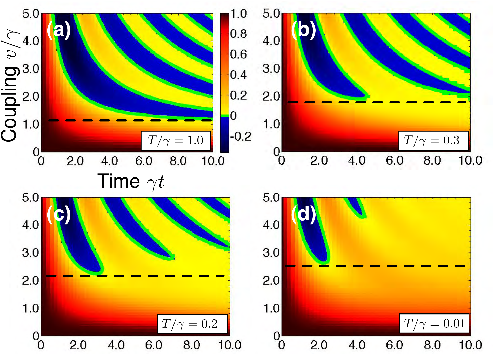
To illustrate these points, we have plotted the time-evolution of $D(t)$ [excluding a trivial phase factor] as a function of the coupling-strength $v$ for various temperatures [Fig. 3]. At high temperatures, visibility oscillations set in at $v_{c}^{q}/\gamma\approx 1$, whereas for $T\rightarrow 0$ [Fig. 3(a)] the first zero-crossing appears only at $v_{c}^{q}/\gamma\approx 2.7$.

Temperature-dependence of strong-coupling threshold.– As explained above, the visibility oscillations are a genuinely non-Gaussian effect. We characterize the onset of the strong coupling regime by the temperature-dependent critical coupling $v_{c}^{q}(T)$, beyond which the zeroes in $D(t)$ appear. At a fixed temperature $T$, the critical coupling-strength $v_{c}^{q}$ and the corresponding zero in $D(t)$ at time $t^{*}$ are found numerically by a bisection algorithm. The result is a “phase-diagram” showing the critical coupling $v_{c}^{q}$ as a function of $T$, [Fig. 4]. The curve $v_{c}^{q}(T)$ separates the $v-T$-plane into two regions. At high temperatures $T$ the critical coupling $v_{c}^{q}$ converges to its classical value, $v_{c}^{q}\rightarrow\gamma$ [a slight offset in the plot is due to limited numerical accuracy]. For low $T$, it increases and saturates at a finite value, as $D(t;v,T)$ is continuous in the limit $T\rightarrow 0$, and $D(t;v,T=0)$ still displays oscillations beyond some threshold. This means the equilibrium quantum Nyquist noise of the fluctuator is enough to observe visibility oscillations, in contrast to the strong-coupling regime studied in [37], where only the nonequilibrium shot noise of discrete electrons could yield these effects.

Spin-Echo.– Finally, we investigate the time-evolution of the density matrix of the charge qubit in a spin-echo experiment, commonly employed to filter out low-frequency fluctuations, whose effect is cancelled in such a procedure. Echo protocols were first invented in NMR, but they are by now standard in qubit experiments, particularly in the solid-state, where they are used to fight $1/f$ noise ([38]). At the initial time $t^{\prime}=0$, the qubit is prepared in a superposition of its two eigenstates, $\left|\psi(t_{0})\right\rangle=1/\sqrt{2}(\left|\uparrow\right\rangle+\left|\downarrow\right\rangle)$. Then we let the qubit evolve according to Eq. (2) up to a time $t^{\prime}=t/2$, at which we perform a $\pi$-pulse $e^{i\frac{\pi}{2}\hat{\sigma}_{x}}$ on the qubit, before evolving up to time $t$. Defining $\hat{\mathcal{U}}_{\pm}=\exp[-i(\hat{\mathcal{H}}_{B}\pm v\hat{\mathcal{Q}}/2)t/2]$, we find the qubit’s final density matrix to be (in analogy to Eq. (3)) $D_{{\rm{Echo}}}(t)=\left\langle\hat{\mathcal{U}}_{-}^{\dagger}\hat{\mathcal{U}}_{+}^{\dagger}\hat{\mathcal{U}}_{-}\hat{\mathcal{U}}_{+}\right\rangle$. As before, we can rewrite this as a determinant in the single-particle Hilbert space,

where $\hat{U}_{\pm}$ is the single-particle evolution operator. In Fig. 5 we compare the echo signal with the free evolution. At low temperatures, the fluctuations are purely quantum in origin, yielding a relatively lower weight for small frequencies and thus a decrease in the effectiveness of the spin echo procedure.

Conclusion.– In conclusion, we have studied the decoherence of a qubit subject to quantum telegraph noise. We have calculated the time-evolution of the coherence and found a strong-coupling regime with an oscillatory time-dependence of the coherence that cannot be mimicked by any Gaussian noise source. We have characterized this regime via the appearance of the first zero in the time-evolution of the coherence and summarized the result in a “phase-diagram”. Moreover, we have presented the time-evolution of the echo-signal in a spin-echo experiment and compared it to the coherence. Straightforward extensions of the formulae presented here may be applied to discuss the effects of more sophisticated pulse sequences [39, 40, 41, 42] which are relevant for protecting quantum information storage.