Thermalization in SU(3) gauge theory after a deconfining quench
Abstract
We determine the time evolution of fluctuations of the Polyakov loop after a quench into the deconfined phase of SU(3) gauge theory from a simple classical relativistic Lagrangian. We compare the structure factors, which indicate spinodal decomposition followed by relaxation, to those obtained via Markov Chain Monte Carlo techniques in SU(3) lattice gauge theory. We find that the time when the structure factor peaks diverges like in the long-wavelength limit. This is due to formation of competing Z(3) domains for configurations where the Polyakov loop exhibits non-perturbatively large variations in space, which delay thermalization of long wavelength modes. For realistic temperatures, and away from the extreme weak-coupling limit, we find that even modes with on the order of experience delayed thermalization. Relaxation times of very long wavelength modes are found to be on the order of the size of the system; thus, the dynamics of competing domains should accompany the hydrodynamic description of the deconfined vacuum.
I Introduction
Relativistic Heavy-Ion Collision (RHIC) experiments carried out at Brookhaven National Laboratory (BNL) provide support for the existence of a quark-gluon plasma (QGP) phase of QCD [1]. In this phase color charges are liberated (deconfined), contrary to the low temperature phase that confines color charges inside colorless objects such as hadrons or glueballs. The existence of confined and deconfined phases has been demonstrated numerically in Lattice Gauge Theory (LGT) studies [2]. Lattice QCD predicts a first-order phase transition for SU(3) pure gauge theory [3] that turns into a crossover for full QCD [4] with physical quark masses.
A collision of two heavy nuclei at high energy releases a large number of gluons from the wave functions of the colliding nuclei [5]. Those gluons interact and eventually form a thermalized QCD plasma with a temperature in excess of the critical temperature for deconfinement. Complete (and consistent) theoretical understanding of the thermalization process is presently lacking. Baier, Mueller, Schiff and Son developed the so-called “bottom-up” approach [6], which is a framework for understanding the processes leading to thermalization and for calculating the thermalization time of the QCD medium as well as its initial temperature (see, however, the critique in ref. [7]). The “bottom-up” approach is based on solving the Boltzmann equation for quasi-particles in a trivial vacuum and neglects the structure of the deconfined phase of the non-Abelian gauge theory arising from the Z(3) center symmetry discovered by t’ Hooft and Polyakov [8]. Below, we shall show that in a model which allows for non-perturbatively large variations of Polyakov loops in space, domain walls form which separate regions of different Z(3) orientation [9]. The competition between such domains affects the thermalization of long-wavelength modes of the Polyakov loop. We shall also provide some model estimates for the relevant wave lengths and time scales.
We adopt a simplified picture where a relativistic heavy-ion collision is viewed as a quench that instantly heats the system to a temperature above the deconfining temperature. The response of Polyakov loop Structure Factors (SFs) to such a heating quench has been studied in SU(3) LGT by Markov Chain Monte Carlo (MCMC) simulations for Glauber (dissipative) dynamics [10]. As unambiguous signals for the transition one finds a dynamical growth of the SF, reaching maxima which scale approximately with the volume, a behavior often characterized as spinodal decomposition [11].
Glauber (model A) dynamics [12] imitates the thermal fluctuation of Nature. It is therefore expected to describe the dissipative features of the transition from one equilibrium ensemble to another well. MCMC updating with a Metropolis or heatbath algorithm falls into the universality class of model A. Such SU(3) MCMC simulations converge to 3D equilibrium ensembles, which are the same as in Minkowski space, because the fourth extension of the Euclidean lattice serves only to define the temperature. The major drawback of Glauber dynamics is not the 4D Euclidean formulation but that it is non-relativistic and, more importantly, that one does not know how to connect the MCMC updating step to a physical time scale.
It was stressed in [13] that relaxation to the vacuum ensemble at high temperature becomes feasible only after each SF has overcome its maximum value. For SU(3) gauge theory this relaxation time diverges with increasing system size due to competing order-order domains with different Z(3) center group triality, which are similar to order-order domains in a 3-state Potts model [14]. This divergence is well known in condensed matter physics [15]. Hence, one should not a-priori exclude the possibility that, under heating, the long wavelength modes in the system do not equilibrate but instead get stuck in the neighborhood of the SF maxima.
In this paper we explore heating quenches into the deconfined phase within Pisarski’s effective model of Polyakov loops [16] (see also ref. [17] for similar effective potential models), which we compare to those from Glauber dynamics. The solutions of the effective theory are obtained through Molecular Dynamics (MD) simulations of hyperbolic, relativistic Minkowski dynamics [18] for which the time scale of the updating step is known (simulations based on a Langevin approach with statistical noise and friction have also been performed, see ref. [19]).
II Effective Model of Polyakov Loops
In Pisarski’s model [16] the deconfined phase of a pure gauge theory is described as a condensate of Polyakov loops. The Z(3)-symmetric effective potential for Polyakov loops (complex for SU(3)) with cubic and quartic interactions takes the form
| (1) |
The energy scale is set by , and the mass coefficient is temperature dependent, while and are constants. These couplings can be chosen so that they reproduce lattice data for the SU(3) pressure and energy density above . A reasonable fit follows with , , and , where and . A plot is shown in fig. 1 of ref. [20].
To complete the effective theory in Minkowski space-time, a kinetic term has to be added:
| (2) |
Here, we assume a Lorentz-invariant form, , and take the coefficient from that for spatial variations of SU(3) Wilson lines [16], with . Thus the dynamics of Polyakov loops is in an intermediate regime between very weak () and very strong () coupling.
We employ a simulation procedure similar to the one of ref. [18] but focus on heating quenches of the system and not on its subsequent cooling [21]; also, we consider here a static, non-expanding metric. Polyakov loop fields are defined on the sites of a spatial cubic lattice of size with periodic boundary conditions. They are initialized in the confined phase at time . Then the temperature entering the effective Lagrangian (2) is set to a value above the deconfinement transition , where the Z(3) center symmetry is spontaneously broken. At temperatures the effective potential takes the shape shown in Fig. 1. In the plane below we show equal height contours.
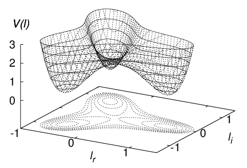
After the quench to the system evolves in time according to the Euler-Lagrange equations derived from the Lagrangian (2) and rearranges itself to a new equilibrium ensemble with non-zero Polyakov loop, which signals symmetry breaking in the infinite volume limit.
In the following we describe how the initial field configurations are constructed.
II.1 Initialization of the field
Introducing real and imaginary parts, we write the Polyakov loop as
| (3) |
We split the fields into a long- and a short wavelength part,
| (4) |
The system is initialized in the unstable confined phase, thus
| (5) |
The initial fluctuations are assumed to be Gaussian,
| (6) |
Consequently, , and hold.
II.2 Counterterms in the equations of motion
In terms of and , the potential can be written as:
| (7) |
Using eq. (4) and averaging over the distribution of initial fluctuations (6) up to order gives the one-loop correction to the effective potential:
| (8) | |||||
The additional second term, which arises from the classical initial fluctuations, needs to be subtracted in order to restore the original potential (7) for the long wavelength modes of the Polyakov loop. The equations of motion including these counterterms are given by
| (9) |
where we replaced with because the difference in the equations of motion is of order and can be neglected. In the simulation we take so that the counterterms simplify to
| (10) | |||||
| (11) |
The numerical results shown below were obtained with ; gives similar results (our statistical errors are larger than the systematic errors due to variation of the initial fluctuations within this range). We do not have a good quantitative estimate for the magnitude of fluctuations, but it appears reasonable to expect that over a length scale of order (see the next section) they should be small compared to unity. On the other hand, the value is still sufficiently large to allow for a relatively rapid onset of the domain formation process, as will be seen in section III.
II.3 Coarse graining
A physical length scale is introduced through coarse graining of the initial field configuration. For example, a simple algorithm amounts to replacing the field at a given site by an average over a subvolume (box) of size :
| (12) |
In physical units, the correlation length at should be on the order of (away from the extreme weak-coupling limit), and we set the lattice spacing by . Dividing eqs. (10,11) by shows that a different scale for the initial correlation length corresponds to rescaling .
The coarse-graining procedure does not affect the long wavelength part of but reduces the fluctuations,
| (13) |
Therefore, the counterterms in (10,11) no longer match the state of the system after coarse-graining. One needs to restore the desired fluctuations by rescaling the initial fields to
| (14) |
so that . These fields are taken as initial configuration which is then propagated in time by solving the equations of motion.
II.4 Dynamics after a temperature quench
To perform a quench the temperature is set to a value in the deconfined phase. Then we use the leapfrog algorithm [22] to integrate the Euler-Lagrange equations (10), (11) in time with the initial conditions described previously. At time , the structure function is defined by the Fourier transformation of the Polyakov loop:
| (15) |
For a fixed value of , is called SF. SFs are our primary observables. In what follows, we label SFs similarly as in [10]:
| (16) | |||||
| (17) | |||||
| (18) |
where denotes the size of the lattice in physical units. Note the relation for . Measurements for include the permutations , and for the permutations , .
III Numerical Results
We quench to several temperatures in the deconfining phase , 1.75, 2.00, 2.25, 2.50 on lattices with spatial extent , 48, 64, 80, 96. Periodic boundary conditions are applied and averaging is done over ensembles of 200 replica. Our length scale set by coarse-graining is fm, corresponding to the SU(3) phase transition temperature of MeV [3]. Using for the correlation length the lattice spacing
| (19) |
follows. Physical volumes in our simulations are , , , and fm3. To reduce finite size effects we take lattices that accommodate at least 10 correlation lengths . When we study different physical volumes, has to be the same for all lattices and is a reasonable value. With, say, we would have to work on larger lattices.

In Fig. 2 we present several SF modes from our Glauber dynamics study [10] on a lattice (quench to , corresponding to , average over 170 replica) for comparison with SF modes from the Minkowski dynamics on a lattice (quench to , average over 200 replica) presented in Fig. 3. The scale on the vertical axis of Fig. 2 differs from that of Fig. 3 because the former has been determined from the bare Polyakov loop while the effective Lagrangian (2) deals with the renormalized loop. The renormalization constant for the Polyakov loop [23] amounts to a constant multiplying the SF. Since we are not interested in this renormalization here, this constant is of minor importance.
Qualitatively, the SFs display the same behavior: an initial exponential growth is followed by equilibration after the lowest SF mode reaches its maximum. As for Glauber dynamics, we interpret this as formation of competing order-order domains between regions of different Z(3) triality [9], whose equilibration takes a long time. For the Minkowskian dynamics the maxima of the lowest SF mode are compiled in Table 1. In the normalization of eq. (15) they scale with volume in the same way as for Glauber dynamics, provided the volumes are large enough. Fits to the form are shown in Fig. 4. Interestingly, both Figs. 2 and 3 show that the above-mentioned effects due to non-perturbatively large variations of the Z(3) phase in space are visible even for modes with . This may be related to Z(3) domain walls forming just after the quench being quite broad (disordered phase) and domains not much larger than .

| 12(1) | 24(2) | 60(4) | 107(7) | 231(16) | |
| 15(1) | 29(2) | 71(6) | 122(8) | 252(16) | |
| 15(1) | 30(2) | 74(5) | 123(8) | 256(17) | |
| 16(1) | 29(2) | 79(5) | 133(9) | 257(18) | |
| 17(1) | 28(2) | 79(5) | 139(10) | 249(17) |

Since the kinetic term in the Lagrangian (2) is assumed to be Lorentz invariant, units for time are the same as for length (apart from the speed of light factor ). When integrating hyperbolic equations, one uses time steps smaller than the spatial lattice spacing . We chose and, therefore, in physical units
| (20) |
We ran trajectories from 15000 to 25000 time steps corresponding to a range from 27.6 fm/c to 46 fm/c.
For the case shown in Fig. 3 the structure factor for the first mode takes about 8 fm/c to reach its maximum, and another fm/c until that mode equilibrates. On the other hand, the second and third modes grow for a shorter period of time and subsequently equilibrate more rapidly. Note that there is an initial lag of fm/c, where growth of SFs is only visible on a logarithmic scale; the precise time for the onset of growth may be sensitive to the spectrum and magnitude of initial fluctuations.
| 5.0(1.2) | 6.3(1.9) | 8.2(1.3) | 11.1(1.4) | 14.0(1.1) | |
| 5.4(1.1) | 6.4(1.9) | 9.5(1.4) | 12.0(1.3) | 15.2(1.2) | |
| 5.0(1.8) | 7.0(1.5) | 10.1(1.3) | 13.2(1.2) | 16.4(1.0) | |
| 5.7(1.5) | 7.4(1.5) | 10.9(1.3) | 14.4(1.1) | 19.1(0.9) | |
| 6.1(1.5) | 7.9(1.4) | 11.9(1.3) | 16.2(1.1) | 19.1(0.9) |
In Table 2 we compile the times needed to reach the maxima of for different volumes and quench temperatures. Evidently, the times before the lowest modes of the system equilibrate can be quite large, in units on the order of the size of the system. Note also that increases with because the barriers between order-order domains grow higher and are more difficult to overcome. This is expected to change for full QCD with light quarks where the Z(3) symmetry is broken explicitly.

Typical trajectories of the volume-averaged Polyakov loop are shown in Fig. 5, together with contours of the potential from Fig. 1. Some of the configurations in the ensemble relax directly towards one of the Z(3) minima, while others get stuck in-between for rather long times. The latter situation corresponds to the case when there are competing domains of approximately equal size: the relaxation of the long-wavelength modes is delayed when the Polyakov loop exhibits non-perturbatively large variations in space. The circle of radius about the origin indicates the average time . Note that for some trajectories the volume-averaged Polyakov loop (the total “magnetization”) can at still be far from one of the minima of the potential. Individual configurations exhibit rather large fluctuations about the mean, as shown in Fig. 6.


For Glauber dynamics it is known [15] that for sufficiently large systems and corresponding wavelengths scales as
| (21) |
For Minkowski dynamics fits to this form are satisfactory, too, as shown in Fig. 7. Thus, in the long wavelength limit the equilibration time for a mode with wave vector is proportional to . The behavior (21) could be used to scale for from table 2 into the corresponding for higher modes via the relation . For , for example, we obtain fm-1 (and fm, which corresponds to the “lag” mentioned above). However, given the rather large statistical error bars shown in Fig. 7 we cannot exclude a linear dependence,
| (22) |
with or without an initial “lag” , either.
IV Conclusions and Outlook
The particle spectrum of a quantum field theory at finite temperature builds upon the phase of its vacuum ensemble, and the structure of the vacuum is fundamental for the dynamics of relaxation processes to equilibrium. In SU(N) gauge theory, non-perturbatively large variations of the Z(N) phase within domain walls arise during the conversion from a confined to a deconfined vacuum ensemble. We find that the Minkowskian dynamics of a simple model for SU(3) Polyakov loops (which incorporates the Z(3) structure of the deconfined vacuum) reproduces the qualitative features of a previous study [10] of Glauber dynamics within LGT reasonably well. Heating above drives the SU(3) gauge theory system from the disordered into the ordered phase. The initial process of spinodal decomposition is signaled by an exponential growth of the SFs. Ordering of the system proceeds through formation of domains of different Z(3) triality until one of them eventually occupies the whole system (see Fig. 5).
For realistic, sub-asymptotic temperatures as relevant for high-energy heavy-ion collisions we find that the rather slow dynamics of competing domains (of the Polyakov loop) delays thermalization of modes with nearly up to . In future, it would be interesting to quantify the contribution of these modes to the bulk viscosity.
Our model for Minkowskian dynamics allows us to estimate a physical time scale for the vacuum conversion process. The relaxation times found in this way for SU(3) pure gauge theory increase as (for sufficiently low ) and are estimated to be on the order of the size of the system for and fm. The hydrodynamic equations describing the evolution of long-wavelength perturbations in a deconfined medium should therefore be extended to account for the dynamics of competing domains of the Polyakov loop.
The model for the dynamics of Polyakov loops could be improved in many ways. As an example, (1) deals only with the trace of the Polyakov loop in the fundamental representation and neglects magnetic fields. Effective Lagrangians which include all degrees of freedom of SU(N) loops as well as magnetic fields (in the static limit) have been proposed recently [24]. Also, the kinetic term from (2) for non-equilibrium configurations, for which we have assumed a Lorentz-invariant form, is in fact not known. Further, one may worry about the importance of quantum corrections to the dynamics of domain walls. Finally, it would be interesting to include the effects due to dynamical quarks, which break the center symmetry explicitly. They reduce the SF maxima and decrease the relaxation time, as has been demonstrated qualitatively for the 3D 3-state Potts model [25] in an external magnetic field, while counter effects may come from the accompanying decrease of the transition temperature and the transformation of the phase transition into a crossover [4].
To improve the simulations, one could drop the assumption of instantaneous quenching and replace it by the thermalization time of the hard modes. The spinodal decomposition process starts already during the quench when the central rapidity volume heats up, and it occurs in an expanding medium where the longitudinal wave vectors experience a red-shift [6]. Moreover, boundary conditions in heavy-ion collisions are not periodic as used in this paper; rather, the surrounding vacuum is confined and therefore disordered. This increases the width and the effective temperature for the deconfinement transition in a volume-dependent way. In a SU(3) equilibrium study the increase in temperature was found to be in the range from 20% for a volume of to 5% for a volume of [26].
Due to all of the above caveats, our numbers should be viewed only as rough first estimates. Nevertheless, it appears that away from the extreme weak-coupling limit () the dynamics of competing domains will influence thermalization of long wavelength modes, perhaps even for not very far below , and hence cannot be neglected.
Acknowledgements
We thank Rob Pisarski for fruitful discussions, and Brookhaven National Laboratory for its hospitality. This work was in part supported by DOE grants DE-FG02-97ER-41022, DE-FC02-06ER-41439 and NSF grant 0555397.
References
- [1] I. Arsene et al. [BRAHMS Collaboration], Nucl. Phys. A 757 (2005) 1; B. B. Back et al., Nucl. Phys. A 757 (2005) 28; J. Adams et al. [STAR Collaboration], Nucl. Phys. A 757 (2005) 102; K. Adcox et al. [PHENIX Collaboration], Nucl. Phys. A 757 (2005) 184.
- [2] L.D. McLerran and B. Svetitsky, Phys. Lett. B 98 (1981) 195; J. Kuti, J. Polonyi and K. Szlachanyi, Phys. Lett. B 98 (1981) 199; J. Engels, F. Karsch, I. Montvay and H. Satz, Nucl. Phys. B 205 (1982) 545.
- [3] G. Boyd, J. Engels, F. Karsch, E. Laermann, C. Legeland, M. Lütgemeier, and B. Petersson, Nucl. Phys. B 469 (1996) 419, and references therein.
- [4] Z. Fodor, Proc. Science, 42 (Lattice 2007) 011; F. Karsch, Proc. Science, 42 (Lattice 2007) 015.
- [5] See, for example, M. Gyulassy and L. McLerran, Nucl. Phys. A 750 (2005) 30.
- [6] R. Baier, A. H. Mueller, D. Schiff and D. T. Son, Phys. Lett. B 502 (2001) 51.
- [7] P. Arnold, J. Lenaghan and G. D. Moore, JHEP 0308 (2003) 002.
- [8] G. ’t Hooft, Nucl. Phys. B 138 (1978) 1; Nucl. Phys. B 153 (1979) 141; A. M. Polyakov, Phys. Lett. B 72 (1978) 477.
- [9] T. Bhattacharya, A. Gocksch, C. Korthals Altes and R. D. Pisarski, Nucl. Phys. B 383 (1992) 497; C. P. Korthals Altes, Nucl. Phys. B 420 (1994) 637; C. Korthals-Altes, A. Kovner and M. A. Stephanov, Phys. Lett. B 469 (1999) 205; P. Giovannangeli and C. P. Korthals Altes, Nucl. Phys. B 608 (2001) 203; Nucl. Phys. B 721 (2005) 1; Nucl. Phys. B 721 (2005) 25; P. de Forcrand, M. D’Elia and M. Pepe, Phys. Rev. Lett. 86 (2001) 1438; P. de Forcrand and L. von Smekal, Phys. Rev. D 66 (2002) 011504; P. de Forcrand and D. Noth, Phys. Rev. D 72 (2005) 114501; P. de Forcrand, C. Korthals-Altes and O. Philipsen, Nucl. Phys. B 742 (2006) 124.
- [10] A. Bazavov, B.A. Berg, and A. Velytsky, Phys. Rev. D 74 (2006) 014501.
- [11] T.R. Miller and M.C. Ogilvie, Phys. Lett. B 488 (2000) 313; Nucl. Phys. B (Proc. Suppl.) 94 (2001) 419. As in these references we use the terminology “spinodal decomposition” in a broader sense than some statistical physicists do.
- [12] R.J. Glauber, J. Math. Phys. 4 (1963) 294. Model A in the classification of P.M. Chaikin and T.C. Lubensky, Principles of condensed matter physics, Cambridge University Press, Cambridge 1997, Table 8.61.1, p.467.
- [13] A. Bazavov, B.A. Berg, and A. Velytsky, Proc. Science 32 (Lattice 2006) 127.
- [14] B. Svetitsky and L.G. Yaffe, Nucl. Phys. B 210 (1982) 423.
- [15] P.M. Chaikin and T.C Lubensky, p.484 (ref. [12]).
- [16] R.D. Pisarski, Phys. Rev. D 62 (2000) 111501(R); A. Dumitru and R. D. Pisarski, Phys. Lett. B 504, 282 (2001); Phys. Rev. D 66 (2002) 096003.
- [17] A.J. Mizher, E.S. Fraga, G. Krein, Braz. J. Phys. 37 (2007) 605; N.C. Cassol-Seewald, R.L.S. Farias, E.S. Fraga, G. Krein, and R.O. Ramos, arXiv:0711.1866v1.
- [18] O. Scavenius, A. Dumitru, and A.D. Jackson, Phys. Rev. Lett. 87 (2001) 182302.
- [19] E. S. Fraga, G. Krein and A. J. Mizher, Phys. Rev. D 76 (2007) 034501.
- [20] O. Scavenius, A. Dumitru and J. T. Lenaghan, Phys. Rev. C 66 (2002) 034903.
- [21] E.T. Tomboulis and A. Velytsky, Phys. Rev. D 72 (2005) 074509 and references therein.
- [22] D. Frenkel and B. Smit, Understanding Molecular Simulation, Academic Press, 2002.
- [23] O. Kaczmarek, F. Karsch, P. Petreczky and F. Zantow, Phys. Lett. B 543 (2002) 41; A. Dumitru, Y. Hatta, J. Lenaghan, K. Orginos and R. D. Pisarski, Phys. Rev. D 70 (2004) 034511; S. Gupta, K. Hübner and O. Kaczmarek, Phys. Rev. D 77 (2008) 034503.
- [24] A. Vuorinen and L. G. Yaffe, Phys. Rev. D 74 (2006) 025011; R. D. Pisarski, Phys. Rev. D 74 (2006) 121703; Ph. de Forcrand, A. Kurkela and A. Vuorinen, arXiv:0801.1566 [hep-ph].
- [25] B.A. Berg, H. Meyer-Ortmanns, and A. Velytsky, Phys. Rev. D 70 (2004) 054505.
- [26] A. Bazavov and B.A. Berg, Phys. Rev. D 76 (2007) 014502.