Network-based consensus averaging with general noisy channels
| Ram Rajagopal∗ | Martin J. Wainwright∗,† | |
|---|---|---|
| ramr@eecs.berkeley.edu | wainwrig@stat.berkeley.edu |
| Department of Statistics†, and |
|---|
| Department of Electrical Engineering and Computer Sciences∗ |
| University of California, Berkeley |
| Berkeley, CA 94720 |
Technical Report
Department of Statistics, UC Berkeley
Keywords: Distributed averaging; sensor networks; message-passing; consensus protocols; gossip algorithms; stochastic approximation; graph Laplacian.
Abstract
This paper focuses on the consensus averaging problem on graphs under general noisy channels. We study a particular class of distributed consensus algorithms based on damped updates, and using the ordinary differential equation method, we prove that the updates converge almost surely to exact consensus for finite variance noise. Our analysis applies to various types of stochastic disturbances, including errors in parameters, transmission noise, and quantization noise. Under a suitable stability condition, we prove that the error is asymptotically Gaussian, and we show how the asymptotic covariance is specified by the graph Laplacian. For additive parameter noise, we show how the scaling of the asymptotic MSE is controlled by the spectral gap of the Laplacian.
1 Introduction
Consensus problems, in which a group of nodes want to arrive at a common decision in a distributed manner, have a lengthy history, dating back to seminal work from over twenty years ago [8, 5, 18]. A particular type of consensus estimation is the distributed averaging problem, in which a group of nodes want to compute the average (or more generally, a linear function) of a set of values. Due to its applications in sensor and wireless networking, this distributed averaging problem has been the focus of substantial recent research. The distributed averaging problem can be studied either in continuous-time [16], or in the discrete-time setting (e.g., [13, 19, 6, 3, 9]). In both cases, there is now a fairly good understanding of the conditions under which various distributed averaging algorithms converge, as well as the rates of convergence for different graph structures.
The bulk of early work on consensus has focused on the case of perfect communication between nodes. Given that noiseless communication may be an unrealistic assumption for sensor networks, a more recent line of work has addressed the issue of noisy communication links. With imperfect observations, many of the standard consensus protocols might fail to reach an agreement. Xiao et al. [20] observed this phenomenon, and opted to instead redefine the notion of agreement, obtaining a protocol that allows nodes to obtain a steady-state agreement, whereby all nodes are able to track but need not obtain consensus agreement. Schizas et al. [17] study distributed algorithms for optimization, including the consensus averaging problem, and establish stability under noisy updates, in that the iterates are guaranteed to remain within a ball of the correct consensus, but do not necessarily achieve exact consensus. Kashyap et al. [12] study consensus updates with the additional constraint that the value stored at each node must be integral, and establish convergence to quantized consensus. Fagnani and Zampieri [10] study the case of packet-dropping channels, and propose various updates that are guaranteed to achieve consensus. Yildiz and Scaglione [21] suggest coding strategies to deal with quantization noise, but do not establish convergence. In related work, Aysal et al [3] used probabilistic forms of quantization to develop algorithms that achieve consensus in expectation, but not in an almost sure sense.
In the current paper, we address the discrete-time average consensus problem for general stochastic channels. Our main contribution is to propose and analyze simple distributed protocols that are guaranteed to achieve exact consensus in an almost sure (sample-path) sense. These exactness guarantees are obtained using protocols with decreasing step sizes, which smooths out the noise factors. The framework described here is based on the classic ordinary differential equation method [15], and allows for the analysis of several different and important scenarios, namely:
- •
Noisy storage: stored values at each node are corrupted by noise, with known covariance structure.
- •
Noisy transmission: messages across each edge are corrupted by noise, with known covariance structure.
- •
Bit constrained channels: dithered quantization is applied to messages prior to transmission.
To the best of our knowledge, this is the first paper to analyze protocols that can achieve arbitrarily small mean-squared error (MSE) for distributed averaging with noise. By using stochastic approximation theory [4, 14], we establish almost sure convergence of the updates, as well as asymptotic normality of the error under appropriate stability conditions. The resulting expressions for the asymptotic variance reveal how different graph structures—ranging from ring graphs at one extreme, to expander graphs at the other—lead to different variance scaling behaviors, as determined by the eigenspectrum of the graph Laplacian [7].
The remainder of this paper is organized as follows. We begin in
Section 2 by describing the distributed averaging
problem in detail, and defining the class of stochastic algorithms
studied in this paper. In Section 3, we state our main
results on the almost-sure convergence and asymptotic normality of our
protocols, and illustrate some of their consequences for particular
classes of graphs. In particular, we illustrate the sharpness of our
theoretical predictions by comparing them to simulation results, on
various classes of graphs. Section 4 is devoted to the
proofs of our main results, and we conclude the paper with discussion
in Section 5. (This work was presented in part at the
Allerton Conference on Control, Computing and Communication in
September 2007.)
Comment on notation: Throughout this paper, we use the following standard asymptotic notation: for a functions and , the notation means that for some constant ; the notation means that for some constant , and means that and .
2 Problem set-up
In this section, we describe the distributed averaging problem, and specify the class of stochastic algorithms studied in this paper.
2.1 Consensus matrices and stochastic updates
Consider a set of nodes, each representing a particular sensing and processing device. We model this system as an undirected graph , with processors associated with nodes of the graph, and the edge set representing pairs of processors that can communicate directly. For each node , we let be its neighborhood set.
Suppose that each vertex makes a real-valued measurement , and consider the goal of computing the average . We assume that for all , as dictated by physical constraints of sensing. For iterations , let represent an -dimensional vector of estimates. Solving the distributed averaging problem amounts to having converge to , where is the vector of all ones. Various algorithms for distributed averaging [16, 6] are based on symmetric consensus matrices with the properties:
| (1a) | |||||
| (1b) | |||||
| (1c) | |||||
The simplest example of such a matrix is the graph Laplacian, defined as follows. Let be the adjacency matrix of the graph , i.e. the symmetric matrix with entries
| (2) |
and let where is the degree of node . Assuming that the graph is connected (so that for all ), the graph Laplacian is given by
| (3) |
Our analysis applies to the (rescaled) graph Laplacian, as well as to various weighted forms of graph Laplacian matrices [7].
Given a fixed choice of consensus matrix , we consider the following family of updates, generating the sequence of -dimensional vectors. The updates are designed to respect the neighborhood structure of the graph , in the sense that at each iteration, the estimate at a receiving node is a function of only11 1 In fact, our analysis is easily generalized to the case where depends only on vertices , where is a (possibly random) subset of the full neighborhood set . However, to bring our results into sharp focus, we restrict attention to the case . the estimates associated with transmitting nodes in the neighborhood of node . In order to model noise and uncertainty in the storage and communication process, we introduce random variables associated with the transmission link from to ; we allow for the possibility that , since the noise structure might be asymmetric.
With this set-up, we consider algorithms that generate a stochastic sequence in the following manner:
1. At time step , initialize for all . 2. For time steps , each node computes the random variables (4) where is the communication-noise function defining the model. 3. Generate estimate as (5) where denotes the Hadamard (elementwise) product between matrices, and is a decaying step size parameter.
2.2 Communication and noise models
It remains to specify the form of the the function that
controls the communication and noise model in the local computation
step in equation (4).
Noiseless real number model: The simplest model, as considered by the bulk of past work on distributed averaging, assumes noiseless communication of real numbers. This model is a special case of the update (4) with , and
| (6) |
Additive edge-based noise model (): In this model, the term is zero-mean additive random noise variable that is associated with the transmission , and the communication function takes the form
| (7) |
We assume that the random variables
and are independent for
distinct edges and , and identically
distributed with zero-mean and variance
.
Additive node-based noise model (): In this model, the function takes the same form (7) as the edge-based noise model. However, the key distinction is that for each , we assume that
| (8) |
where is a single noise variable associated
with node , with zero mean and variance . Thus, the random variables
and
are all identical for all edges out-going from the transmitting
node .
Bit-constrained communication (): Suppose that the channel from node to is bit-constrained, so that one can transmit at most bits, which is then subjected to random dithering. Under these assumptions, the communication function takes the form
| (9) |
where represents the -bit quantization function with maximum value and is random dithering. We assume that the random dithering is applied prior to transmission across the channel out-going from vertex , so that is the same random variable across all neighbors .
3 Main result and consequences
In this section, we first state our main result, concerning the stochastic behavior of sequence generated by the updates (5). We then illustrate its consequences for the specific communication and noise models described in Section 2.2, and conclude with a discussion of behavior for specific graph structures.
3.1 Statement of main result
Consider the factor that drives the updates (5). An important element of our analysis is the conditional covariance of this update factor, denoted by and given by
| (10) |
A little calculation shows that the element of this matrix is given by
| (11) |
Moreover, the eigenstructure of the consensus matrix plays an important role in our analysis. Since it is symmetric and positive semidefinite, we can write
| (12) |
where be an orthogonal matrix with columns defined by unit-norm eigenvectors of , and is a diagonal matrix of eigenvalues, with
| (13) |
It is convenient to let denote the matrix with columns defined by eigenvectors associated with positive eigenvalues of — that is, excluding column , associated with the zero-eigenvalue . With this notation, we have
| (14) |
Theorem 1.
Consider the random sequence generated by the update (5) for some communication function , consensus matrix , and step size parameter .
- (a)
In all cases, the sequence is a strongly consistent estimator of , meaning that almost surely (a.s.).
- (b)
Theorem 1(a) asserts that the sequence is a strongly consistent estimator of the average. As opposed to weak consistency, this result guarantees that for almost any realization of the algorithm, the associated sample path converges to the exact consensus solution. Theorem 1(b) establishes that for appropriate choices of consensus matrices, the rate of MSE convergence is of order , since the -rescaled error converges to a non-degenerate Gaussian limit. Such a rate is to be expected in the presence of sufficient noise, since the number of observations received by any given node (and hence the inverse variance of estimate) scales as . The solution of the Lyapunov equation (16) specifies the precise form of this asymptotic covariance, which (as we will see) depends on the graph structure.
3.2 Some consequences
Theorem 1 can be specialized to particular noise and communication models. Here we derive some of its consequences for the , and models. For any model for which Theorem 1(b) holds, we define the average mean-squared error as
| (17) |
corresponding to asymptotic error variance, averaged over nodes of the graph.
Corollary 1 (Asymptotic MSE for specific models).
Given a consensus matrix with second-smallest eigenvalue , the sequence is a strongly consistent estimator of the average , with asymptotic MSE characterized as follows:
- (a)
For the additive edge-based noise () model (7):
(18) - (b)
Proof.
The essential ingredient controlling the asymptotic MSE is the conditional covariance matrix , which specifies via the Lyapunov equation (16). For analyzing model , it is useful to establish first the following auxiliary result. For each , we have
| (20) |
where is the spectral norm (maximum eigenvalue for a positive semdefinite symmetric matrix). To see this fact, note that
Since satisfies the Lyapunov equation, we have
Note that the diagonal entries of the matrix are of the form . The difference between the RHS and LHS matrices constitute a positive semidefinite matrix, which must have a non-negative diagonal, implying the claimed inequality (20).
In order to use the bound (20), it remains to
compute or upper bound the spectral norm ,
which is most easily done using the elementwise
representation (11).
(a) For the model (7), we have
| (21) |
Since we have assumed that the random variables on each edge are i.i.d., with zero-mean and variance , we have
Consequently, from the elementwise expression (11), we conclude that is diagonal, with entries
so that , which establishes the
claim (18).
(b) For the model (9), we have
| (22) |
where is the quantization noise. Therefore, we have , and using the fact that consists of eigenvectors of (and hence also , the Lyapunov equation (16) takes the form
which has the explicit diagonal solution with entries . Computing the asymptotic MSE yields the claim (19). The proof of the same claim for the model is analogous. ∎
3.3 Scaling behavior for specific graph classes
We can obtain further insight by considering Corollary 1 for specific graphs, and particular choices of consensus matrices . For a fixed graph , consider the graph Laplacian defined in equation (3). It is easy to see that is always positive semi-definite, with minimal eigenvalue , corresponding to the constant vector. For a connected graph, the second smallest eigenvector is strictly positive [7]. Therefore, given an undirected graph that is connected, the most straightforward manner in which to obtain a consensus matrix satisfying the conditions of Corollary 1 is to rescale the graph Laplacian , as defined in equation (3), by its second smallest eigenvalue , thereby forming the rescaled consensus matrix
| (23) |
with .
With this choice of consensus matrix, let us consider the implications of Corollary 1(b), in application to the additive node-based noise () model, for various graphs. We begin with a simple lemma, proved in Appendix A, showing that, up to constants, the scaling behavior of the asymptotic MSE is controlled by the second smallest eigenvalue .
Lemma 1.
Combined with known results from spectral graph theory [7], Lemma 1 allows us to make specific predictions about the number of iterations required, for a given graph topology of a given size , to reduce the asymptotic MSE to any : in particular, the required number of iterations scales as
| (25) |
Note that this scaling is similar but different from the scaling of noiseless updates [6, 9], where the MSE is (with high probability) upper bounded by for , which scales as
| (26) |
for a decaying spectral gap .
3.4 Illustrative simulations
We illustrate the predicted scaling (25) by some simulations on different classes of graphs. For all experiments reported here, we set the step size parameter . The additive offset serves to ensure stability of the updates in very early rounds, due to the possibly large gain specified by the rescaled Laplacian (23). We performed experiments for a range of graph sizes, for the additive node noise () model (8), with noise variance in all cases. For each graph size , we measured the number of iterations required to reach a fixed level of mean-squared error.
3.4.1 Cycle graph
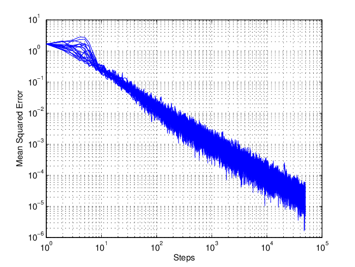
Consider the ring graph on vertices, as illustrated in Figure 2(a). Panel (b) provides a log-log plot of the MSE versus the iteration number ; each trace corresponds to a particular sample path. Notice how the MSE over each sample coverges to zero. Moreover, since Theorem 1 predicts that the MSE should drop off as , the linear rate shown in this log-log plot is consistent. Figure 2(c) plots the number of iterations (vertical axis) required to achieve a given constant MSE versus the size of the ring graph (horizontal axis). For the ring graph, it can be shown (see Chung [7]) that the second smallest eigenvalue scales as , which implies that the number of iterations to achieve a fixed MSE for a ring graph with vertices should scale as . Consistent with this prediction, the plot in Figure 2(c) shows a quadratic scaling; in particular, note the excellent agreement between the theoretical prediction and the data.
 |
 |
 |
|---|---|---|
| (a) | (b) | (c) |
3.4.2 Lattice model
Figure 3(a) shows the two-dimensional four nearest-neighbor lattice graph with vertices, denoted . Again, panel (b) corresponds to a log-log plot of the MSE versus the iteration number , with each trace corresponding to a particular sample path, again showing a linear rate of convergence to zero. Panel (c) shows the number of iterations required to achieve a constant MSE as a function of the graph size. For the lattice, it is known [7] that , which implies that the critical number of iterations should scale as . Note that panel (c) shows linear scaling, again consistent with the theory.
 |
 |
 |
|---|---|---|
| (a) | (b) | (c) |
3.4.3 Expander graphs
Consider a bipartite graph , with vertices and edges joining only vertices in to those in , and constant degree ; see Figure 4(a) for an illustration with . A bipartite graph of this form is an expander [1, 2, 7] with parameters , if for all subsets of size , the neighborhood set of —namely, the subset
has cardinality . Intuitively, this property guarantees that each subset of , up to some critical size, “expands” to a relatively large number of neighbors in . (Note that the maximum size of is , so that close to guarantees that the neighborhood size is close to its maximum, for all possible subsets .) Expander graphs have a number of interesting theoretical properties, including the property that —that is, a bounded spectral gap [1, 7].
In order to investigate the behavior of our algorithm for expanders, we construct a random bi-partite graph as follows: for an even number of nodes , we split them into two subsets , each of size . We then fix a degree , construct a random matching on nodes, and use it connect the vertices in to those in . This procedure forms a random bipartite -regular graph; using the probabilistic method, it can be shown to be an edge-expander with with probability , as the graph size tends to infinity [1, 11].
 |
 |
 |
|---|---|---|
| (a) | (b) | (c) |
Given the constant spectral gap , the scaling in number of iterations to achieve constant MSE is . This theoretical prediction is compared to simulation results in Figure 4; note how the number of iterations soon settles down to a constant, as predicted by the theory.
4 Proof of Theorem 1
We now turn to the proof of Theorem 1. The basic idea is to relate the behavior of the stochastic recursion (5) to an ordinary differential equation (ODE), and then use the ODE method [15] to analyze its properties. The ODE involves a function , with its specific structure depending on the communication and noise model under consideration. For the and models, the relevant ODE is given by
| (27) |
For the model, the approximating ODE is given by
| (28) |
In both cases, the ODE must satisfy the initial condition .
4.1 Proof of Theorem 1(a)
The following result connects the discrete-time stochastic process to the deterministic ODE solution, and establishes Theorem 1(a):
Lemma 2.
Proof.
We prove this lemma by using the ODE method and stochastic approximation—in particular, Theorem 1 from Kushner and Yin [14], which connects stochastic recursions of the form (5) to the ordinary differential equation . Using the definition of in terms of , for the and models, we have
from which we conclude that with the stepsize choice , we have
By our assumptions on the eigenstructure of , the system is globally asymptotically stable, with a line of fixed points . Given the initial condition , we conclude that is the unique asymptotically fixed point of the ODE, so that the claim (29) follows from Kushner and Yin [14].
For the model, the analysis is somewhat more involved, since the quantization function saturates the output at . For the dithered quantization model (9), we have
where is the saturation function (28). We now claim that is also the unique asymptotically stable fixed point of the ODE subject to the initial condition . Consider the eigendecomposition , where . Define the rotated variable , so that the ODE (28) can be re-written as
| (30a) | |||||
| (30b) | |||||
where denotes the column of .
Note that , since it is associated with the eigenvalue . Consequently, the solution to equation (30a) takes the form
| (31) |
with unique fixed point , where is the average value,
A fixed point for equations (30b) requires that , for . Given that the columns of form an orthogonal basis, this implies that for some constant , or equivalently (given the connection )
| (32) |
Given the piecewise linear nature of the saturation function, this equality implies either that the fixed point satisfies the elementwise inequality (if ); or the elementwise inequality (if ); or as the final option, the when . But from equation (31), we know that . But we also have by definition, so that putting together the pieces yields
| (33) |
Thus the only possibility is that for some constant , and the relation implies that , which establishes the claim. ∎
4.2 Proof of Theorem 1(b)
We analyze the update (5) using results from Benveniste et al [4]. In particular, given the stochastic iteration , define the expectation , its Jacobian matrix , and the covariance matrix . Then Theorem 3 (p. 110) of Benveniste et al [4] asserts that as long as the eigenvalues are strictly below . then
| (34) |
where the covariance matrix is the unique solution to the Lyapunov equation
| (35) |
We begin by computing the conditional distribution ; for the models and it takes the form
| (36) |
since the conditional expectation of the random matrix is given by . For the model, since the quantization is finite with maximum value , the expectation is given by
| (37) |
where the saturation function was defined previously (28). In addition, we computed form of the the covariance matrix previously (10). Finally, we note that
| (38) |
for all three models. (This fact is immediate for models and ; for the model, note that Theorem 1(a) guarantees that falls in the middle linear portion of the saturation function.)
We cannot immediately conclude that asymptotic normality (34) holds, because the matrix has a zero eigenvalue (). However, let us decompose where is the matrix with unit norm columns as eigenvectors, and . Let denote the matrix obtained by deleting the first column of . Defining the vector , we can rewrite the update in -dimensional space as
| (39) |
for which the new effective function is given by , with . Since by assumption, the asymptotic normality (34) applies to this reduced iteration, so that we can conclude that
where solves the Lyapunov equation
We conclude by noting that the asymptotic covariance of is related to that of by the relation
| (40) |
from which Theorem 1(b) follows.
5 Discussion
This paper analyzed the convergence and asymptotic behavior of distributed averaging algorithms on graphs with general noise models. Using suitably damped updates, we showed that it is possible to obtain exact consensus, as opposed to approximate or near consensus, even in the presence of noise. We guaranteed almost sure convergence of our algorithms under fairly general conditions, and moreover, under suitable stability conditions, we showed that the error is asymptotically normal, with a covariance matrix that can be predicted from the structure of the consensus operator. We provided a number of simulations that illustrate the sharpness of these theoretical predictions. Although the current paper has focused exclusively on the averaging problem, the methods of analysis in this paper are applicable to other types of distributed inference problems, such as computing quantiles or order statistics, as well as computing various types of -estimators. Obtaining analogous results for more general problems of distributed statistical inference is an interesting direction for future research.
Acknowledgements
This work was presented in part at the Allerton Conference on Control, Computing and Communication, September 2007. Work funded by NSF-grants DMS-0605165 and CCF-0545862 CAREER to MJW. The authors thank Pravin Varaiya and Alan Willsky for helpful comments.
Appendix A Proof of Lemma 1
We begin by noting that for the normalized graph Laplacian , it is known that for any graph, the second smallest eigenvalue satisfies the upper bound . Moreover, we have . See Lemma 1.7 in Chung [7] for proofs of these claims.
Using these facts, we establish Lemma 1 as follows. Recall that by construction, we have , so that the second smallest eigenvalue of is , and the remaining eigenvalues are greater than or equal to one. Applying Corollary 1 to the model, we have
using the fact that .
In the other direction, using the fact that and the bound for . we have
References
- [1] N. Alon. Eigenvalues and expanders. Combinatorica, 6(2):83–96, 1986.
- [2] N. Alon and J. Spencer. The Probabilistic Method. Wiley Interscience, New York, 2000.
- [3] T. C. Aysal, M. Coates, and M. Rabbat. Distributed average consensus using probabilistic quantization. In IEEE Workshop on Stat. Sig. Proc., Madison, WI, August 2007.
- [4] A. Benveniste, M. Metivier, and P. Priouret. Adaptive Algorithms and Stochastic Approximations. Springer-Verlag, New York, NY, 1990.
- [5] V. Borkar and P. Varaiya. Asymptotic agreement in distributed estimation. IEEE Trans. Auto. Control, 27(3):650–655, 1982.
- [6] S. Boyd, A. Ghosh, B. Prabhakar, and D. Shah. Randomized gossip algorithms. IEEE Transactions on Information Theory, 52(6):2508–2530, 2006.
- [7] F.R.K. Chung. Spectral Graph Theory. American Mathematical Society, Providence, RI, 1991.
- [8] M. H. deGroot. Reaching a consensus. Journal of the American Statistical Association, 69(345):118–121, March 1974.
- [9] A. G. Dimakis, A. Sarwate, and M. J. Wainwright. Geographic gossip: Efficient averaging for sensor networks. IEEE Trans. Signal Processing, 53:1205–1216, March 2008.
- [10] F. Fagnani and S. Zampieri. Average consensus with packet drop communication. SIAM J. on Control and Optimization, 2007. To appear.
- [11] J. Feldman, T. Malkin, R. A. Servedio, C. Stein, and M. J. Wainwright. LP decoding corrects a constant fraction of errors. IEEE Trans. Information Theory, 53(1):82–89, January 2007.
- [12] A. Kashyap, T. Basar, and R. Srikant. Quantized consensus. Automatica, 43:1192–1203, 2007.
- [13] D. Kempe, A. Dobra, and J. Gehrke. Gossip-based computation of aggregate information. Proc. 44th Ann. IEEE FOCS, pages 482–491, 2003.
- [14] H. J. Kushner and G. G. Yin. Stochastic Approximation Algorithms and Applications. Springer-Verlag, New York, NY, 1997.
- [15] L. Ljung. Analysis of recursive stochastic algorithms. IEEE Transactions in Automatic Control, 22:551–575, 1977.
- [16] R. Olfati-Saber, J. A. Fax, and R. M. Murray. Consensus and cooperation in networked multi-agent systems. Proceedings of the IEEE, 95(1):215–233, 2007.
- [17] I. D. Schizas, A. Ribeiro, and G. B. Giannakis. Consensus in ad hoc WSNs with noisy links: Part I distributed estimation of deterministic signals. IEEE Transactions on Signal Processing, 56(1):350–364, 2008.
- [18] J. Tsitsiklis. Problems in decentralized decision-making and computation. PhD thesis, Department of EECS, MIT, 1984.
- [19] L. Xiao and S. Boyd. Fast linear iterations for distributed averaging. Systems & Control Letters, 52:65–78, 2004.
- [20] L. Xiao, S. Boyd, and S.-J. Kim. Distributed average consensus with least-mean-square deviation. Journal of Parallel and Distributed Computing, 67(1):33–46, 2007.
- [21] M. E. Yildiz and A. Scaglione. Differential nested lattice encoding for consensus problems. In Info. Proc. Sensor Networks (IPSN), Cambridge, MA, April 2007.