The exact tree amplitudes for the scattering of strings in flat spacetime can be obtained in many ways. For example, the path integral for the sum over worldsheets can be completely evaluated by choosing a parametrization that linearizes the worldsheet equations. Because of this, one doesn’t really need a visualization of the “classical” worldsheet that would represent a saddle-point approximation to the path integral. But for string scattering on non-trivial backgrounds, for which an exact evaluation is not possible, the saddle-point approximation is frequently the only available approach to calculations. Then it becomes important to understand the physical meaning of various classical worldsheet solutions.

Because of the AdS/CFT correspondence [1], the scattering of field quanta of a conformal quantum field theory is dual to string scattering on an Anti-deSitter spacetime, and the strong ’t Hooft coupling limit on the field side is dual to the classical limit on the string side. For example, Alday and Maldacena (AM) [2, 3] have employed this duality to calculate the scattering of gluons and their superpartners in ${\cal N}=4$ supersymmetric Yang-Mills theory in the limit of strong coupling. This limit is described by the classical dynamics of string moving in an Anti-deSitter (AdS) spacetime. To describe the scattering one needs to find the classical worldsheet in Poincaré coordinates $x^{\mu}(\xi),z(\xi)$, with its boundary at $z=\infty$.³³ 3 Here $\xi=(\xi^{0},\xi^{1})$ are the 2D worldsheet coordinates of the string. Actually, it is easier to work with T-dual coordinates [4, 5] $y^{\mu}(\xi)$ and to use $r=R^{2}/z$ instead of $z$. These coordinates turn out to be the Poincaré coordinates of another AdS manifold. In terms of them, the boundary of the desired worldsheet is at $r=0$, and, for the scattering of $n$ ground state strings, the boundary conditions are simply that the worldsheet end at $r=0$ on a closed polygon of $n$ lightlike line segments, given by the momenta of the $n$ external particles [2].

One can also use T-dual coordinates to describe string scattering in flat spacetime. This is usually not done, but we think it a useful and interesting exercise to examine the T-dual description of worldsheets in this case as well. In flat spacetime, choosing conformally flat worldsheet coordinates linearizes the equations of motion, and the worldsheet solution can be expressed in terms of Green functions, with appropriate boundary conditions, for the 2D Laplacian. Studying the solutions in flat spacetime helps clarify the physical nature of the boundary conditions used by AM in the worldsheet solutions on AdS applied to gluon scattering at strong coupling. For example, the scattering amplitudes can be explicitly related to finite time transition amplitudes in the lightcone gauge, and therefore can be obtained from a reduction formalism. In particular, it is interesting to compare the flat and AdS worldsheets as a way to illuminate the very different physics in the two cases: in the flat case the string tension $T_{0}$ is a constant implying that the energy of a stretched string is proportional to its length, whereas in the AdS case the effective tension depends on $z$, $T_{\rm eff}(z)$, dropping to 0 at $z=\infty$ (or $r=0$). The vanishing tension in the second case implies a continuous mass spectrum of string excitations which complicates the application of the reduction formalism (as with all theories with massless particles).

Thus in this article we set out to study the worldsheets appropriate to various scattering processes in both flat and AdS spacetime. In AdS, exact solutions for string motion are hard to come by. We look at the solutions used by AM for scattering of gluons by gluons, which were constructed from earlier ones found by Kruczenski [6], as well as a more general solution involving a gluon scattering off some kind of external source. This latter process, however, does not look like a gluon scattering from a heavy quark represented on AdS by a string stretching from a point at $z=0$ out to $z=\infty$, a process we had hoped to understand. Instead, for this solution the end of the string interacting with the source is at $z=\infty$ ($r=0$).

In all cases we display the solutions in the T-dual coordinates $y^{\mu}(\sigma,\tau)$ and, in the case of AdS, $r$. These coordinates are particularly nice because the interesting worldsheets are of finite extent in them, and they can be displayed graphically in a striking way. In the case of on-shell gluon scattering, the Minkowski part of the worldsheet in AdS is at first glance qualitatively very similar to the flat space worldsheet. The very different physics can only be understood after considering the quantitative differences due to the dynamics of the AdS radius $r$. We also find worldsheets for a gluon scattering from a 0-brane or a 1-brane in flat spacetime. These can be compared to the more general solution in AdS mentioned at the end of the previous paragraph, and we study them to gain insight into the physics of the latter solution.

The rest of the paper is organized as follows. The next two sections provide background for the subsequent studies. In section 2 we discuss the T-duality transformation from the point of view of the phase-space action principle. Section 3 gives a brief discussion of the properties of the “single gluon” defined by AM using a 3-brane at fixed finite $z_{IR}$. We begin those studies in section 4 which discusses the worldsheets appropriate to $n$ string scattering in flat space. All our solutions in AdS₅ are constructed from exact solutions on an AdS₃ submanifold that are found and described in section 5. Then section 6 discusses in this general framework the AdS₅ solution for 4 gluon scattering used by AM. Section 7 discusses a new solution in AdS₅ that describes a single gluon scattering from an external source. Section 8 employs lightcone gauge to compare the physics of the AdS 4-string solutions to that of the flat space solutions. Finally, to gain further insight into such external source scattering processes we study the worldsheets for scattering of a string off 0-brane and 1-brane sources in flat space in section 9. We include one appendix on useful facts about various covariant and lightcone worldsheet parametrizations, and a second on the relation between conformal transformations in 4 dimensional spacetime and isometry transformations of AdS₅.

We choose coordinates for AdS spacetime so that the line element is $ds^{2}={R^{2}}(dx_{\mu}dx^{\mu}+dz^{2})/z^{2}$. Then the worldsheet action for a string moving on AdS₅ is in Nambu-Goto form⁴⁴ 4 in this section we use ^. and ^′ to represent ${\partial\over\partial\xi^{0}}$ and ${\partial\over\partial\xi^{1}}$, respectively.

$\displaystyle S_{NG}$

$\displaystyle=$

$\displaystyle-T_{0}\int d^{2}\xi{R^{2}\over z^{2}}\sqrt{({\dot{x}}\cdot x^{\prime}+{\dot{z}}z^{\prime})^{2}-({\dot{x}}^{2}+{\dot{z}}^{2})(x^{\prime 2}+z^{\prime 2})}.$

(1)

With the introduction of a dynamical worldsheet metric $g_{\alpha\beta}$ we get an equivalent form

$\displaystyle S_{ws}\equiv\int d^{2}\xi{\cal L}=-{T_{0}\over 2}\int d^{2}\xi\sqrt{g}g^{\alpha\beta}{R^{2}\over z^{2}}(\partial_{\alpha}x\cdot\partial_{\beta}x+\partial_{\alpha}z\partial_{\beta}z).$

(2)

For ${\cal N}=4$ super Yang-Mills, the AdS/CFT correspondence gives $T_{0}R^{2}=\sqrt{g^{2}N_{c}/4\pi^{2}}=\sqrt{\lambda}$. The momenta conjugate to $(x^{\mu},z)$ are $({\cal P}^{\mu},\Pi)=-R^{2}T_{0}\sqrt{g}g^{0\beta}\partial_{\beta}(x^{\mu},z)/z^{2}$. Then the canonical hamiltonian density is

	$\displaystyle{\cal H}$	$\displaystyle=$	$\displaystyle{\dot{x}}\cdot{\cal P}+{\dot{z}}\Pi-{\cal L}$		(3)
		$\displaystyle=$	$\displaystyle{\kappa\over 2}\left({z^{2}\over T_{0}R^{2}}({\cal P}^{2}+\Pi^{2})+{T_{0}R^{2}\over z^{2}}(x^{\prime 2}+z^{\prime 2})\right)+\mu(x^{\prime}\cdot{\cal P}+z^{\prime}\Pi),$
	$\displaystyle\kappa$	$\displaystyle=$	$\displaystyle-{1\over g^{00}\sqrt{g}},\qquad\mu=-{g^{01}\over g^{00}}.$		(4)

If, instead, the canonical momentum is obtained from the Nambu-Goto action (1), ${\cal H}$ and the coefficients of $\kappa$, $\mu$ are identically zero.This represents phase space constraints for which $\kappa$, $\mu$ are then introduced as Lagrange multipliers. In either case, the phase space Lagrange density is [7, 8]

	$\displaystyle{\cal L}$	$\displaystyle=$	$\displaystyle{\dot{x}}\cdot{\cal P}+{\dot{z}}\Pi-{\kappa\over 2}\left({z^{2}\over T_{0}R^{2}}({\cal P}^{2}+\Pi^{2})+{T_{0}R^{2}\over z^{2}}(x^{\prime 2}+z^{\prime 2})\right)-\mu(x^{\prime}\cdot{\cal P}+z^{\prime}\Pi)$		(5)
		$\displaystyle\to$	$\displaystyle{\dot{x}}\cdot{\cal P}-{\kappa\over 2}\left({z^{2}\over T_{0}R^{2}}{\cal P}^{2}+{T_{0}R^{2}\over z^{2}}x^{\prime 2}\right)-\mu x^{\prime}\cdot{\cal P}+{R^{2}T_{0}\over 2z^{2}}\left[{({\dot{z}}-\mu z^{\prime})^{2}\over\kappa}-\kappa z^{\prime 2}\right],$		(6)

where in the second line we have eliminated $\Pi$ using its purely algebraic equation of motion. To discuss duality we simply replace ${\cal P}=q^{\prime}\equiv T_{0}y^{\prime}$:

$\displaystyle{\cal L}$

$\displaystyle=$

$\displaystyle T_{0}\left({\dot{x}}\cdot y^{\prime}-{\kappa\over 2}\left({z^{2}\over R^{2}}y^{\prime 2}+{R^{2}\over z^{2}}x^{\prime 2}\right)-\mu(x^{\prime}\cdot y^{\prime})+{R^{2}\over 2z^{2}}\left[{({\dot{z}}-\mu z^{\prime})^{2}\over\kappa}-\kappa z^{\prime 2}\right]\right)$

(7)

and we immediately see a symmetry up to surface terms under $x\leftrightarrow q/T_{0}=y$, $z\to R^{2}/z$. This is T-duality. In the form written in (7), ${\cal L}$ gives a good action principle for the variable $x$. Note that the absence of ${\dot{y}}$ in ${\cal L}$ implies a gauge symmetry under $y\to y+f(\xi^{0})$. Varying $y$ with open string topology implies $y^{\prime}=R^{2}(\dot{x}-\mu x^{\prime})/(\kappa z^{2})$. Then varying $x$ gives

$\displaystyle{\dot{y}}^{\prime}=\left[{\kappa R^{2}\over z^{2}}x^{\prime}+\mu y^{\prime}\right]^{\prime},\qquad\left[{\kappa R^{2}\over z^{2}}x^{\prime}+\mu y^{\prime}\right]_{\rm ends}=0.$

(8)

Thus this version of the action principle implies the duality transformation in the form

$\displaystyle y^{\prime}={R^{2}\over\kappa z^{2}}(\dot{x}-\mu x^{\prime}),\qquad{\dot{y}}={\kappa R^{2}\over z^{2}}x^{\prime}+\mu y^{\prime}+f(\xi^{0})={\kappa R^{2}\over z^{2}}x^{\prime}+\mu{R^{2}\over\kappa z^{2}}(\dot{x}-\mu x^{\prime})+f(\xi^{0})$

(9)

with undetermined $f(\xi^{0})$, which can, if desired, be removed by a gauge transformation, giving

$\displaystyle y^{\prime}={R^{2}\over\kappa z^{2}}(\dot{x}-\mu x^{\prime}),\qquad{\dot{y}}-\mu y^{\prime}={\kappa R^{2}\over z^{2}}x^{\prime}.$

(10)

Also notice that the free-end boundary conditions on $x$ imply ${\dot{y}}_{\rm ends}=f(\xi^{0})$ which implies that $d{\Delta{y}}/d\xi^{0}=0$, where $\Delta y$ is the difference in the values of $y$ at the two ends. In a gauge where $f(\xi^{0})=0$ $y$ satisfies Dirichlet conditions ${\dot{y}}_{\rm ends}=0$ at the ends.

Next consider Dirichlet conditions on $x$, ${\dot{x}}_{\rm ends}=0$. Then

$\displaystyle{y^{\prime}}_{\rm ends}=-{R^{2}\mu\over\kappa z^{2}}x^{\prime}=-{\mu\over\kappa^{2}}({\dot{y}}-\mu y^{\prime}-f(\xi^{0}))$

(11)

which, in a gauge where $f(\xi^{0})=0$, are precisely analogous to the free end condition on $x$. This condition would follow as a free end condition on $y$ from the action obtained from (7) by substituting ${\dot{x}}\cdot y^{\prime}\to{\dot{y}}\cdot x^{\prime}$. Indeed, this substitution must be made to get a good action principle for the variable $y$. We find

$\displaystyle{\dot{x}}\cdot y^{\prime}-{\dot{y}}\cdot x^{\prime}={\partial\over\partial\xi^{0}}({x}\cdot y^{\prime})-{\partial\over\partial\sigma}({x}\cdot{\dot{y}})=-{\partial\over\partial\xi^{0}}({y}\cdot x^{\prime})+{\partial\over\partial\sigma}({y}\cdot{\dot{x}})$

(12)

so the substitution is achieved by adding a surface term to the action. Doing this and reversing the logic, we conclude that the Nambu-Goto form of the action for the T-dual variables $y$ is

$\displaystyle{\tilde{S}}_{NG}$

$\displaystyle=$

$\displaystyle-T_{0}\int d^{2}\xi{R^{2}\over r^{2}}\sqrt{({\dot{y}}\cdot y^{\prime}+{\dot{r}}r^{\prime})^{2}-({\dot{y}}^{2}+{\dot{r}}^{2})(y^{\prime 2}+r^{\prime 2})}.$

(13)

Either action principle has identical consequences for the dual pair $x,y$ modulo the gauge invariance appropriate to the action chosen.

For closed-string topology, these duality results will follow if we only require $y^{\prime}$ to be periodic, allowing $y$ to shift by a function of $\xi^{0}$ upon traversing a period: that is $y$ is required to be periodic up to a gauge transformation.

Finally we determine the worldsheet metric in terms of the $x,z$ or the $y=q/T_{0},r\equiv R^{2}/z$ by varying the action with respect to $\kappa,\mu$, and using the duality relations (with $f(\xi^{0})=0$):

	$\displaystyle\mu$	$\displaystyle=$	$\displaystyle{{\dot{x}}\cdot x^{\prime}+{\dot{z}}\cdot z^{\prime}\over x^{\prime 2}+z^{\prime 2}}\ =\ {{\dot{y}}\cdot y^{\prime}+{\dot{r}}\cdot r^{\prime}\over y^{\prime 2}+r^{\prime 2}},$		(14)
	$\displaystyle\kappa^{2}$	$\displaystyle=$	$\displaystyle{({\dot{x}}\cdot x^{\prime}+{\dot{z}}z^{\prime})^{2}-({\dot{x}}^{2}+{\dot{z}}^{2})(x^{\prime 2}+z^{\prime 2})\over(x^{\prime 2}+z^{\prime 2})^{2}}\ =\ {({\dot{y}}\cdot y^{\prime}+{\dot{r}}r^{\prime})^{2}-({\dot{y}}^{2}+{\dot{r}}^{2})(y^{\prime 2}+r^{\prime 2})\over(y^{\prime 2}+r^{\prime 2})^{2}}.$		(15)

Alday and Maldacena were principally interested in using the AdS/CFT correspondence to study the scattering of gluons in ${\cal N}=4$ supersymmetric Yang-Mills theory. For purposes of comparing to work of Bern, Dixon, and Smirnov (BDS) [9] they needed to define on-shell amplitudes with a definite number of gluons at strong coupling. Strictly speaking all these amplitudes are zero due to infrared divergences: the non-vanishing physical observables are jets with an indefinite number of gluons. Thus an IR cutoff that enables the definition of single gluon states is needed. One practical infrared cutoff is to use dimensional regularization, continuing to $D=4+\epsilon$. This is used by BDS in their perturbative calculations, which establish the definition of single gluons using the dressed gluon propagator.

However the notion of a dressed single-gluon propagator is obscure in the string description. Instead AM define single gluons as open AdS strings with ends moving on a D3 brane at fixed $z=z_{IR}<\infty$. They then take $z_{IR}\to\infty$ after continuing to $D=4+\epsilon$ dimensions. In the string description the IR divergences are due to the huge degeneracy of single open-string mass eigenstates when the effective rest tension vanishes as $z_{IR}\to\infty$.⁵⁵ 5 At finite $z_{IR}$ a string with ends fixed at finite $z_{IR}$ has an energy gap at $N=\infty$ (see [10, 11, 12]). This is the string dual to the huge degeneracy in the field description due to the presence of many massless gluons. Fixing the ends of the open string representing a gluon to $z=z_{IR}$ breaks this degeneracy by introducing an energy cost to stretching an open string with ends fixed to the brane. It is not a confining energy cost (it stays finite at infinite separation of the string ends), but a finite classical energy cost is enough to discretize the semi-classical energy near zero, producing a gap which enables the lowest mass eigenstate, which is the ${\cal N}=4$ supermultiplet containing the gluon, to be filtered out by the reduction formalism.

At strong coupling the string dynamics is classical, and it is significant that the unstretched classical open string (i.e. $x^{\prime}=0$ for all $\xi^{1}$), corresponding to the ground state of the string and identified with the gluon, solves the full set of classical AdS string equations at constant $z$: ${\dot{z}}=z^{\prime}=0$. Such a solution requires ${\dot{x}}\cdot{\dot{x}}=0$, i.e. the unstretched open string moves freely on the brane at the speed of light—it is a massless point particle. In T-dual variables this condition reads $y^{\prime}\cdot y^{\prime}=0$. In other words the reduction formalism applied at finite $z_{IR}$ (which supplies a mass gap) will require the classical worldsheet in T-dual space for gluon scattering amplitudes to end at $z=z_{IR}$ on light-like line segments corresponding to the momenta of the on-shell gluons. This is precisely the prescription employed by Alday and Maldacena.

If $z_{IR}$ is finite the open string modeling the single gluon has internal structure that can be analyzed semi-classically. Indeed, the model is mathematically equivalent to the models of $Q{\bar{Q}}$ mesons studied in the context of AdS/CFT inspired models of QCD. For example, in [13] the rotational motion of such an open string, with ends fixed to a 3-brane at fixed $z$ is solved numerically. An interesting outcome of that work is the leading Regge trajectory $J(E^{2})$, described by a straight open string rotating rigidly about its midpoint. The asymptotic behavior of the trajectory at small $E$ and near ionization threshold, which we translate to the gluon parameters, was obtained analytically. For $E\sim 0$, it behaves linearly with $E^{2}$: $J(E^{2})\sim\alpha^{\prime}E^{2}z_{IR}^{2}/R^{2}$. That is, the AdS open string for finite $z_{IR}$ behaves like a massless relativistic string at low energy [7]. The effective tension of this slightly stretched string is $T_{\rm eff}=T_{0}R^{2}/z_{IR}^{2}$ and drops to zero when the IR cutoff is removed, $z_{IR}\to\infty$, causing the mass spectrum to become continuous from zero. At higher energy the energy spectrum shows a threshold $E_{I}=R^{2}/(\pi\alpha^{\prime}z_{IR})$ at which there is an accumulation of energy levels. $J$ becomes infinite as $E\to E_{I}$ from below, in a manner similar to the Bohr levels in hydrogen just below ionization threshold. Specifically, $E(J)\sim E_{I}(1-\alpha^{2}/(8J^{2}))$, where $\alpha=4\pi^{2}R^{2}/(\alpha^{\prime}\Gamma(1/4)^{4})$. This behavior at large $J$ agrees with the nonrelativistic model of two particles with equal mass, given by the energy of a static string stretching from $z=z_{IR}$ to $z=\infty$, interacting with a Coulomb potential $-\alpha/r$. Here $\alpha$ is precisely equal to the value predicted by the AdS/CFT correspondence for the $Q{\bar{Q}}$ static force in ${\cal N}=4$ Yang-Mills theory in the strong ’t Hooft coupling limit [10].

We begin our study of classical worldsheets with a translation of known results for scattering of strings in flat Minkowski space to the T-dual description:

$\displaystyle{\partial y^{\mu}\over\partial x}=i{\partial x^{\mu}\over\partial y},\qquad{\partial y^{\mu}\over\partial y}=-i{\partial x^{\mu}\over\partial x},$

(16)

where we parameterize the worldsheet using the upper half complex plane $z=x+iy$. Then for $n$-string scattering we have

	$\displaystyle x^{\mu}(z)$	$\displaystyle=$	$\displaystyle{-i}\sum_{r=1}^{n-1}{(y_{r}-y_{r-1})^{\mu}\over\pi}\log|z-u_{r}|,$		(17)
	$\displaystyle y^{\mu}(z)$	$\displaystyle=$	$\displaystyle\sum_{r=0}^{n-1}{y_{r}^{\mu}\over\pi}\left(\tan^{-1}{u_{r+1}-x\over y}-\tan^{-1}{u_{r}-x\over y}\right).$		(18)

Here the momenta carried by the strings are $p_{r}=y_{r}-y_{r-1}$, and the Koba-Nielsen variable of string $r$ is $u_{r}$. For definiteness we take $0=u_{1}<u_{2}<\cdots<u_{n-1}=1$ and $u_{0}=-\infty$, $u_{n}=\infty$. The $x^{\mu}$ satisfy Neumann conditions $\partial x^{\mu}/\partial y=0$ on the real axis $y=0$ (away from the points $x=u_{r}$), whereas the $y^{\mu}$ satisfy Dirichlet conditions on the real axis: $y^{\mu}(x,0)=y_{r}^{\mu}$ on the interval $u_{r}<x<u_{r+1}$. In T-dual variables the $y^{\mu}$ are discontinuous where the string momenta enter the worldsheet. Specializing to $n=4$:

	$\displaystyle x^{\mu}(z)$	$\displaystyle=$	$\displaystyle{-i}\sum_{r=1}^{3}{(y_{r}-y_{r-1})^{\mu}\over\pi}\log|z-u_{r}|,$		(19)
	$\displaystyle y^{\mu}(z)$	$\displaystyle=$	$\displaystyle{y_{0}^{\mu}\over\pi}\left({\pi\over 2}-\tan^{-1}{x\over y}\right)+{y_{1}^{\mu}\over\pi}\left(\tan^{-1}{u-x\over y}+\tan^{-1}{x\over y}\right)$		(20)
			$\displaystyle+{y_{2}^{\mu}\over\pi}\left(\tan^{-1}{1-x\over y}-\tan^{-1}{u-x\over y}\right)+{y_{3}^{\mu}\over\pi}\left({\pi\over 2}-\tan^{-1}{1-x\over y}\right).$

Strictly speaking, conformal gauge also requires the constraints $(\partial x^{\mu}/\partial x)(\partial x_{\mu}/\partial x)=(\partial x^{\mu}/\partial y)(\partial x_{\mu}/\partial y)$ and $(\partial x^{\mu}/\partial x)(\partial x_{\mu}/\partial y)=0$. These would be expected to hold only on-shell though. For the classical string on-shell means $(y_{i+1}-y_{i})^{2}=0$. But even then these constraints only hold when the Koba-Nielsen variables are at a stationary point of the action, which corresponds to a saddle point of the integration. (For example $u=u_{0}\equiv t/(s+t)$ for the four point function). Away from the saddle point the $u$ integrand is off-shell in the classical sense. Integration over the whole range puts the amplitude on-shell in the quantum sense. Indeed we know that the integrated Koba-Nielsen integrands do satisfy the quantum operator Virasoro constraints. It is interesting that the classical Virasoro constraints do hold, though, at the saddle points.

An interesting feature of the T-dual worldsheet is that it is finite in extent. We display this graphically in Fig. 1. It is striking that, plotted in $y$ space, the boundary of the worldsheet is a finite polygon of lightlike straight line segments.

It is important to realize that in the conformally flat coordinates $x,y$, these segments are the images of points on the $x$ axis—the points where the boundary values of $y$ are discontinuous. Since in the $x,y$ coordinates the problem is just a Dirichlet problem for the Laplace equation, the solution is uniquely determined by the values of $y$ specified on the boundary, even if there are discontinuities in these boundary values. In Fig. 1 the Dirichlet data are just the four corners of the polygon. The reason that the discontinuities in $y^{\mu}$ are mapped to straight lines in this figure is that, in the upper half plane near a discontinuity at say $x+iy=u_{r}$, the different components of $y^{\mu}$ are related to their boundary values by the same Green functions and hence are linearly related to each other. Thus, as $u_{r}$ is approached from different directions in the upper half plane, the solution $y^{\mu}(x,y)$ approaches different points on a straight line joining the two boundary values on either side of $u_{r}$. It might seem strange that giving data at 4 points is enough to determine the solution, but we must remember that if we parametrize the worldsheet with coordinates in $y^{\mu}$-space (e.g. $y^{1},y^{2}$), the equations for the worldsheet are nonlinear and quite different from the Laplace equation.

Next we turn to a consideration of the worldsheet solution found by AM which controls gluon scattering at strong coupling in ${\cal N}=4$ super Yang-Mills theory. We will look in more detail at their method and find additional solutions whose interpretation is quite different.

Starting from the Nambu-Goto action (13) in terms of T-dual variables which we call $y^{\prime\mu},\;r^{\prime}$,⁶⁶ 6 In this section the prime no longer indicates a derivative. we restrict ourselves to AdS₃ and make the Anzatz, closely related to one proposed earlier by Kruczenski [6], and used by AM:

$\displaystyle r^{\prime}=w(\xi^{0})e^{\xi^{0}},\quad y^{\prime 0}=e^{\xi^{0}}\cosh{\xi^{1}},\quad y^{\prime 1}=e^{\xi^{0}}\sinh\xi^{1},\quad y^{\prime 2}=y^{\prime 3}=0.$

(21)

The Lagrangian whose stationary point determines $w(\xi^{0})$ is then

$\displaystyle L=-{\sqrt{1-(w+\dot{w})^{2}}\over w^{2}}$

(22)

and the ensuing Euler-Lagrange equation is

$\displaystyle-{d\over d\xi^{0}}{w+\dot{w}\over w^{2}\sqrt{1-(w+\dot{w})^{2}}}=-{w+\dot{w}\over w^{2}\sqrt{1-(w+\dot{w})^{2}}}-2{\sqrt{1-(w+\dot{w})^{2}}\over w^{3}}$

(23)

where the dot indicates derivative with respect to $\xi^{0}$.

Note that for a static solution, $\dot{w}=0$, we immediately find $w=\pm\sqrt{2}$. For positive $r^{\prime}$ one would take $w=\sqrt{2}$ which is the starting point of AM. To find nonstatic solutions we can use the conservation law that follows from $L$ to find

$\displaystyle E={1-w(w+\dot{w})\over w^{2}\sqrt{1-(w+\dot{w})^{2}}},$

(24)

$\displaystyle\dot{w}={1-w^{2}-E^{2}w^{4}\pm|w|\sqrt{E^{4}w^{4}+(w^{2}-1)E^{2}}\over w(1+E^{2}w^{2})},$

(25)

$\displaystyle{d\xi^{0}\over d|w|}={|w|\over 1-w^{2}}\left[1\pm{|w|\over\sqrt{w^{4}+{(w^{2}-1)/E^{2}}}}\right]..$

(26)

The condition that $({\partial y^{\prime}/\partial\xi^{1}})\cdot({\partial y^{\prime}/\partial\xi^{1}})=0$ at $r^{\prime}=0$ requires that the region $\xi^{0}\rightarrow-\infty$ be part of the solution. For generic $E^{2}$ the singularities arising from the zeros of the square root are integrable, thereby leaving only $|w|\rightarrow 1$ and $|w|\rightarrow\infty$ as possibilities. At large $|w|$ the integrand behaves as $-d|w|/|w|$ implying $\xi^{0}\sim-\log|w|$ or $|w|\sim e^{-\xi^{0}}$. But then $r^{\prime}\sim{\rm O}(1)$. This is not acceptable since, for the application to gluon scattering, we need the corner to be at $r^{\prime}=0$.

We next examine the behavior near $|w|=1$ which is singular only for the upper sign in (26):

$\displaystyle d\xi^{0}\sim-d|w|{1\over|w|-1}=-d\log\left||w|-1|\right|.$

(27)

This singularity corresponds to $\xi^{0}\rightarrow+\infty$. We conclude, therefore, that the solution for generic $E^{2}$ does not include the light-like corner at $r^{\prime}=0$.

For the special case $E^{2}=-1/4$, however, the zeros of the square root in (26) coalesce and the singularity becomes a pole at $|w|=\sqrt{2}$. This corresponds to the desired behavior $\xi^{0}\rightarrow-\infty$. Then (26) becomes

$\displaystyle{d\xi^{0}\over d|w|}=-{|w|(2-|w|)\over(2-w^{2})(|w|-1)}$

(28)

which integrates to

$\displaystyle Ce^{\xi^{0}}={1\over|w|-1}\left(\sqrt{2}-|w|\over\sqrt{2}+|w|\right)^{1/\sqrt{2}}\equiv f(|w|)$

(29)

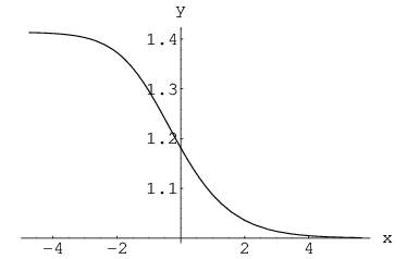
where $C$ is an integration constant. Note that as $C\rightarrow 0$ we obtain the static solution $|w|=\sqrt{2}$. We get a completely different solution by choosing $C=1$ and taking $w>0$ in order that $r^{\prime}\geq 0$. Both solutions have $E^{2}=-1/4$. A plot of $w(\xi^{0})$ for the nonstatic solution is given in Fig. 2.

Note that $w(\xi^{0})$ approaches the static solution $\sqrt{2}$ as $\xi^{0}\rightarrow-\infty$.

It will prove convenient in what follows to replace $\xi^{0}$ as one of the worldsheet parameters by $w$. Then we can write both the static and nonstatic solutions using a common notation. We have

$\displaystyle y^{\prime 0}=f(w){\cosh\xi^{1}},\quad y^{\prime 1}=f(w)\sinh\xi^{1},\quad r^{\prime}=g(w)f(w)$

(30)

where $g(w)=\sqrt{2}$ for the static solution and $g(w)=w$ for the nonstatic solution.

In the previous section we described a worldsheet solution for the dual variables that lies in an AdS₃ subspace of AdS₅ by assuming (30) along with $y^{\prime 2}=y^{\prime 3}=0$. Any such solution can be extended into AdS₅ by means of SO(4,2) rotations and boosts of the embedding coordinates

$\displaystyle Y^{\prime\mu}={R\over r^{\prime}}y^{\prime\mu},\quad Y^{\prime-1}={1\over 2r^{\prime}}(R^{2}+r^{\prime 2}+y^{\prime\mu}y^{\prime}_{\mu}),\quad Y^{\prime 4}={1\over 2r^{\prime}}(R^{2}-r^{\prime 2}-y^{\prime\mu}y^{\prime}_{\mu})$

(31)

which are such that

$\displaystyle(Y^{\prime-1})^{2}-(Y^{\prime 4})^{2}-Y^{\prime\mu}Y^{\prime}_{\mu}=R^{2}.$

(32)

Notice that $Y^{\prime 4}$ and $Y^{\prime-1}$ enter the left side just as space-like and time-like coordinates respectively. Thus we are free to reinterpret the AdS₃ with the relabeling $4\to 1\to 2\to 4$ so that $Y^{\prime 4}=0$ in the new interpretation. Then if we make rotations given by the angle $\theta$ in the (0,-1) plane and $\phi$ in the new (1,2) plane as well as a boost through hyperbolic angle $\alpha$ in the (0,4) plane, we obtain a new dual AdS₅ solution:

$\displaystyle r=R{2r^{\prime}R\over(R^{2}+r^{\prime 2}+y^{\prime\mu}y^{\prime}_{\mu})(\cos\theta+\sin\theta\sinh\alpha)+2y^{\prime 0}R(\sin\theta-\cos\theta\sinh\alpha)}$

(33)

$\displaystyle y^{0}=R{\cosh\alpha[(2y^{\prime 0}R\cos\theta-(R^{2}+r^{\prime 2}+y^{\prime\mu}y^{\prime}_{\mu})\sin\theta]\over(R^{2}+r^{\prime 2}+y^{\prime\mu}y^{\prime}_{\mu})(\cos\theta+\sin\theta\sinh\alpha)+2y^{\prime 0}R(\sin\theta-\cos\theta\sinh\alpha)}$

(34)

$\displaystyle y^{1}=R{(R^{2}-r^{\prime 2}-y^{\prime\mu}y^{\prime}_{\mu})\cos\phi+2y^{\prime 1}R\sin\phi\over(R^{2}+r^{\prime 2}+y^{\prime\mu}y^{\prime}_{\mu})(\cos\theta+\sin\theta\sinh\alpha)+2y^{\prime 0}R(\sin\theta-\cos\theta\sinh\alpha)}$

(35)

$\displaystyle y^{2}=R{2y^{\prime 1}R\cos\phi-(R^{2}-r^{\prime 2}-y^{\prime\mu}y^{\prime}_{\mu})\sin\phi\over(R^{2}+r^{\prime 2}+y^{\prime\mu}y^{\prime}_{\mu})(\cos\theta+\sin\theta\sinh\alpha)+2y^{\prime 0}R(\sin\theta-\cos\theta\sinh\alpha)}$

(36)

$\displaystyle y^{3}=0.$

(37)

More precisely, what we are doing here is viewing the original solution from the point of view of different frames as well as different Poincaré patches.

Ryang [14] has conducted an investigation of the behavior of the solution employed by AM under more general SO(4,2) transformations. AM take $\theta=\phi=\pi/4$ and $\sinh\alpha=v$. In the following, we restrict attention to $\phi=\alpha=0$. Using the AdS₃ Ansatz (30)

$\displaystyle r^{\prime}=g(w)f(w),\quad y^{\prime 0}=f(w)\cosh{\xi^{1}},\quad y^{\prime 1}=f(w)\sinh\xi^{1},\quad y^{\prime 2}=y^{\prime 3}=0$

(38)

we find

$\displaystyle r=R{g(w)\over c(w)\cos\theta+\cosh\xi^{1}\sin\theta}$

(39)

$\displaystyle y^{0}=R{\cosh\xi^{1}\cos\theta-c(w)\sin\theta\over c(w)\cos\theta+\cosh\xi^{1}\sin\theta}$

(40)

$\displaystyle y^{1}=R{-s(w)\over c(w)\cos\theta+\cosh\xi^{1}\sin\theta}$

(41)

$\displaystyle y^{2}=R{\sinh\xi^{1}\over c(w)\cos\theta+\cosh\xi^{1}\sin\theta}$

(42)

$\displaystyle y^{3}=0$

(43)

where

$\displaystyle c(w)={1\over 2}\left(f(w)[\{g(w)\}^{2}-1]+{1\over f(w)}\right),\quad s(w)={1\over 2}\left(f(w)[\{g(w)\}^{2}-1]-{1\over f(w)}\right),$

(44)

We assume that $0\leq\theta\leq\pi/2$ so as to avoid $r<0$ and find, for $g(w)=\sqrt{2}$,

$\displaystyle r=R{\sqrt{2}\over\cosh\xi^{0}\cos\theta+\cosh\xi^{1}\sin\theta}$

(45)

$\displaystyle y^{0}=R{\cosh\xi^{1}\cos\theta-\cosh\xi^{0}\sin\theta\over\cosh\xi^{0}\cos\theta+\cosh\xi^{1}\sin\theta}$

(46)

$\displaystyle y^{1}=R{-\sinh\xi^{0}\over\cosh\xi^{0}\cos\theta+\cosh\xi^{1}\sin\theta}$

(47)

$\displaystyle y^{2}=R{\sinh\xi^{1}\over\cosh\xi^{0}\cos\theta+\cosh\xi^{1}\sin\theta}$

(48)

$\displaystyle y^{3}=0.$

(49)

We illustrate this solution in Figs. 3-5 for several angles $\theta$. Note that in this case $c(w)=\cosh\xi^{0}$ and $s(w)=\sinh\xi^{0}$. For $\pi/4\leq\theta\leq\pi/2$ we can make use of the symmetry under $\theta\leftrightarrow\pi-\theta$, $\xi^{0}\leftrightarrow\xi^{1}$, $y^{1}\leftrightarrow-y^{2}$ and $y^{0}\leftrightarrow-y^{0}$. Notice that when $\theta>0$ these solutions show four corners, but when $\theta=0$ a pair of these corners is sent to infinity, leaving only two corners.

The physical meaning of a solution is found by looking in the Minkowski target space of $y^{\mu}$ at points where $r=0$ (or almost 0). Using (45) we find that $r=0$ when $|\xi^{0}|$ or $|\xi^{1}|$ or possibly both are infinite. There are four cases, where one or the other of $|\xi^{0}|$ and $|\xi^{1}|$ are infinite, with the other finite:

$\displaystyle\xi^{0}\rightarrow\infty:\quad y^{\mu}_{a}=R(-\tan\theta,-\sec\theta,0,0)$

(50)

$\displaystyle\xi^{1}\rightarrow\infty:\quad y^{\mu}_{b}=R(\cot\theta,0,\csc\theta,0)$

(51)

$\displaystyle\xi^{0}\rightarrow-\infty:\quad y^{\mu}_{c}=R(-\tan\theta,\sec\theta,0,0)$

(52)

$\displaystyle\xi^{1}\rightarrow-\infty:\quad y^{\mu}_{d}=R(\cot\theta,0,-\csc\theta,0).$

(53)

In the interpretation of these solutions as describing scattering of glue by glue, the differences of these quantities are proportional to the (incoming) momenta of the massless gluons. We should then have

$\displaystyle(y_{a}-y_{b})^{2}=(y_{b}-y_{c})^{2}=(y_{c}-y_{d})^{2}=(y_{d}-y_{a})^{2}=R^{2}[\sec^{2}\theta+\csc^{2}\theta-(\tan\theta+\cot\theta)^{2}]=0$

(54)

which is indeed the case. Furthermore, we can identify the Mandelstam variables for the gluon scattering process as

$\displaystyle s=-(y_{a}-y_{c})^{2}=-4R^{2}\sec^{2}\theta$

(55)

$\displaystyle t=-(y_{b}-y_{d})^{2}=-4R^{2}\csc^{2}\theta$

(56)

so that $t/s=\cot^{2}\theta$.

Using the duality transformation (10) we can translate this solution to the original coordinate space, with $z=R^{2}/r$ in place of $r$:

$\displaystyle z={R\over\sqrt{2}}(\cosh\xi^{0}\cos\theta+\cosh\xi^{1}\sin\theta)$

(57)

$\displaystyle x^{0}=i{R\over 2}\sinh\xi^{0}\sinh\xi^{1}$

(58)

$\displaystyle x^{1}=i{R\over 2}(\xi^{1}\cos\theta+\cosh\xi^{0}\sinh\xi^{1}\sin\theta)$

(59)

$\displaystyle x^{2}=i{R\over 2}(\xi^{0}\sin\theta+\sinh\xi^{0}\cosh\xi^{1}\cos\theta)$

(60)

$\displaystyle x^{3}=0.$

(61)

Note the world sheet invariance under $\theta\rightarrow\pi/2-\theta$, $\xi^{0}\leftrightarrow\xi^{1}$, $y^{1}\leftrightarrow-y^{2}$, $x^{1}\leftrightarrow x^{2}$. The fact that the coordinates are all imaginary shows that the physical scattering process described is classically inaccessible, analogous to reflection above a barrier in one-dimensional quantum mechanics.

We next examine the properties that follow from using the nonstatic solution in the embedding into AdS₅. This is accomplished by choosing $g(w)=w$. This new solution is given by Eqs. (39)-(43)

$\displaystyle\bar{r}=R{w\over c(w)\cos\theta+\cosh\xi^{1}\sin\theta}$

(62)

$\displaystyle\bar{y}^{0}=R{\cosh\xi^{1}\cos\theta-c(w)\sin\theta\over c(w)\cos\theta+\cosh\xi^{1}\sin\theta}$

(63)

$\displaystyle\bar{y}^{1}=R{-s(w)\over c(w)\cos\theta+\cosh\xi^{1}\sin\theta}$

(64)

$\displaystyle\bar{y}^{2}=R{\sinh\xi^{1}\over c(w)\cos\theta+\cosh\xi^{1}\sin\theta^{\prime}}$

(65)

$\displaystyle\bar{y}^{3}=0.$

(66)

We illustrate the result in Fig. 6 for $\theta=\pi/4$.

What we see are two light-like lines in the $r=0$ hyperplane joined at one corner. They are connected at their other ends by a curve for which $r\neq 0$. However, having made the SO(4,2) transformation it is now meaningful to extend the domain of $w$ to the region $w<1$ where $r$ remains positive.⁷⁷ 7 We thank Martin Kruczenski for stressing this possibility to us. If we do this Fig. 6 now is transformed to Fig. 7.

References

• [1] J. Maldacena, Adv. Theor. Math. Phys. 2, 231 (1998), hep-th/9711200;
S.S. Gubser, I.R. Klebanov and A.M. Polyakov, Phys. Lett. B428, 105 (1998), hep-th/9802109;
E. Witten, Adv. Theor. Math. Phys. 2, 253 (1998), hep-th/9802150.
• [2] L. F. Alday and J. Maldacena, JHEP 0706 (2007) 064 [arXiv:0705.0303 [hep-th]].
• [3] L. F. Alday and J. Maldacena, JHEP 0711 (2007) 068 [arXiv:0710.1060 [hep-th]].
• [4] G. ’t Hooft, Nucl. Phys. B72 (1974) 461.
• [5] K. Bardakci and C. B. Thorn, Nucl. Phys. B 626 (2002) 287 [arXiv:hep-th/0110301].
• [6] M. Kruczenski, JHEP 0212 (2002) 024 [arXiv:hep-th/0210115].
• [7] P. Goddard, J. Goldstone, C. Rebbi and C. B. Thorn, Nucl. Phys. B 56 (1973) 109.
• [8] R. R. Metsaev, C. B. Thorn and A. A. Tseytlin, Nucl. Phys. B 596 (2001) 151 [arXiv:hep-th/0009171].
• [9] Z. Bern, L. J. Dixon and V. A. Smirnov, Phys. Rev. D 72 (2005) 085001 [arXiv:hep-th/0505205].
• [10] S.-J. Rey and J. Yee, hep-th/9803001;
J. Maldacena, Phys. Rev. Lett. 80, 4859 (1998), hep-th/9803002.
• [11] C. G. Callan and A. Guijosa, Nucl. Phys. B 565 (2000) 157 [arXiv:hep-th/9906153].
• [12] I. R. Klebanov, J. Maldacena and C. B. Thorn, JHEP 0604 (2006) 024 [arXiv:hep-th/0602255].
• [13] M. Kruczenski, D. Mateos, R. C. Myers and D. J. Winters, JHEP 0307 (2003) 049 [arXiv:hep-th/0304032].
• [14] S. Ryang, Phys. Lett. B 659 (2008) 894 [arXiv:0710.1673 [hep-th]].
• [15] S. Mandelstam, Nucl. Phys. B 64 (1973) 205.
• [16] C. B. Thorn, Nucl. Phys. B 637 (2002) 272 [Erratum-ibid. B 648 (2003) 457] [arXiv:hep-th/0203167].
• [17] S. Gudmundsson, C. B. Thorn and T. A. Tran, Nucl. Phys. B 649 (2003) 3 [arXiv:hep-th/0209102].