Avalanches, branching ratios, and clustering of attractors in Random Boolean Networks and in the segment polarity network of Drosophila
Abstract
We discuss basic features of emergent complexity in dynamical systems far from equilibrium by focusing on the network structure of their state space. We start by measuring the distributions of avalanche and transient times in Random Boolean Networks (RBNs) and in the Drosophila polarity network by exact enumeration. A transient time is the duration of the transient from a starting state to an attractor. An avalanche is a special transient which starts as single Boolean element perturbation of an attractor state. Significant differences at short times between the avalanche and the transient times for RBNs with small connectivity – compared to the number of elements – indicate that attractors tend to cluster in configuration space. In addition, one bit flip has a non-negligible chance to put an attractor state directly onto another attractor. This clustering is also present in the segment polarity gene network of Drosophila melanogaster, suggesting that this may be a robust feature of biological regulatory networks. We also define and measure a branching ratio for the state space networks and find evidence for a new time scale that diverges roughly linearly with for . Analytic arguments show that this time scale does not appear in the random map nor can the random map exhibit clustering of attractors. We further show that for the branching ratio exhibits the largest variation with distance from the attractor compared to other values of and that the avalanche durations exhibit no characteristic scale within our statistical resolution. Hence, we propose that the branching ratio and the avalanche duration are new indicators for scale-free behavior that may or may not be found simultaneously with other indicators of emergent complexity in extended, deterministic dynamical systems.
pacs
05.45.-a, 89.75.-k, 89.75.Fb, 89.75.Da, 87.18.CfI Introduction
Random Boolean Networks (RBNs) [1] are elementary models for signaling processes such as genetic regulation – where a binary state based on Boolean logic [2, 3, 4] encapsulates local gene expression. The dichotomy between their easy construction and their emergent complex behavior has motivated researchers in diverse fields including the neurological [5], computational [6], evolutionary [7] and physical [8, 9] sciences to use these or related models as test beds for ideas about self-organization.
The most well known fact about RBNs is that they exhibit three distinct phases in a statistical ensemble obtained by averaging over random realizations: chaotic, frozen and critical, depending on the connectivity of the Boolean elements. Derrida and Pomeau [10] used an annealed approximation to prove that is a critical ensemble in between ordered and chaotic regimes. According to their analysis, the distinct phases correspond to different patterns of growth for the Hamming distance between two nearly identical initial states. For the distance on average grows exponentially. For the distance on average decays exponentially. For the ensemble of random realizations is critical - the distance is dominated by fluctuations. The existence of this critical phase has been used to argue that many natural systems, including life itself, function at a so-called “edge of chaos” [11, 12, 13, 14, 15].
However, different measures of criticality, which appear simultaneously in the ensemble of RBNs, may not point to the same critical behavior when applied to real signaling networks. For instance, there may be many distinct “edges of chaos” (according to different definitions of dynamical criticality) that can appear in networks that are not members of a statistical ensemble, but are, instead, organized by natural selection or by other forces. More to the point, we believe that one should not conflate all measures of criticality as being necessarily equivalent in treating complex systems far from equilibrium since there is no reason a priori that they should probe intrinsically related dynamical fluctuations. Hence, weq explore several alternative probes of criticality in RBNs that may be more empirical or, indeed, more useful in revealing the forces and constraints that shape natural or man-made regulatory or signaling processes.
To this end, here we develop new methods of complex network analysis to analyze ensembles of state space networks (SSNs) for RBNs and compare their measurable observables to that of the segment polarity network of Drosophila melanogaster [16] where possible. The aspects of these SSNs that have received most attention so far include the probability distribution of attractor lengths and basins of attraction sizes [17, 18, 19]. In the context of regulatory networks, attractors are thought to correspond to distinct cellular states [11] or cycles [20], while the attractors of a signal transduction network correspond to steady state response(s) to the presence of a given signal [21]. In Ref. [22, 23, 24] some exact results were derived for RBNs with . The critical case of was re-examined numerically in Ref. [25], which reported power law behavior in the distribution of transient times. Ref. [26] examined the probability of returning to the same attractor after perturbing various number of nodes. In Ref. [24] methods of complex network analysis were able to distinguish the (critical) ensemble from the others using measures of network heterogeneity in the SSNs. These network measures include node degree (a local measure) and path diversity (a global measure) as well as variations in the path diversity between different realizations in the statistical ensemble.
Inspired by the idea of self-organized criticality [13], here we start by using avalanches to probe the structure of the SSNs. Avalanches are the responses of a system in an attractor state to small perturbations (a bit flip of a single Boolean element). These eventually die out and the system returns to an attractor state, which will be the same or a different attractor. By exact numeration, we find that the distribution of avalanche times allows a clear distinction between the ensemble and other values of . While the avalanche and transient time distributions converge (except for an overall normalization) at large times, significantly more avalanches of short durations exist compared to transients. This shows that attractors preferentially cluster in configuration space for RBNs for all small compared to the number of elements in the network, . This feature is also found in the Boolean representation of the segment polarity gene network in Drosophila [16]. This biological network has a distribution of avalanche times closer to the ensemble than to other values of .
In order to clarify the differences between avalanches and transients at short times we define a “branching ratio” to descibe how the average number of dynamical states grows as a function of distance from the attractor. The average branching ratio is given by the ratio of the probability distribution for transient times at successive times, . For the quantity crosses unity at a certain distance from the attractor where the SSN is the most “bushy”. The crossing time grows with system size, , indicating a new diverging time scale for RBNs. This scale may also separate the short time regime where the avalanche and transient times differ from the long time regime where they converge.
I.1 Outline
In Section II, we review basic facts about RBNs and define relevant quantities for our analysis. Section III contains results from numerical simulations for RBNs, while Section IV compares the behaviors found with that in the Drosophila segment polarity network. We conclude with a summary in Section V.
II Random Boolean Networks
An RBN consists of Boolean elements where the value of each element evolves in discrete time according to a random Boolean function of distinct input arguments. Each of these arguments is chosen randomly from the Boolean elements of the network. For each set of values of the arguments, the Boolean function is chosen randomly to be with probability (bias) and with probability . The inputs and functions assigned to each element remain fixed for each realization. Ensemble averages are achieved here by considering many different realizations of the Boolean network with and constrained to certain values and for bias, .
The state of the RBN is a bit-vector that specifies the value of each Boolean element. Here we are exclusively concerned with the case of deterministic dynamics achieved by updating all elements of a given RBN in parallel. This uniquely maps each state to one successor state, known as its “image”. Consequently, the dynamics of an RBN can be visualized as a state space network (SSN) [27, 24]. An SSN is made by connecting each of the dynamical states of an RBN to its image with a directed link. The out-degree of each node in the SSN is the number of its images and hence exactly one. The in-degree of a node, which is the number of pre-images of the state, ranges from 0 to in principle. In the context of SSNs, the “distance” between two states or nodes in the network is the length of the shortest path connecting them — if such a path exists. This directly implies that the distance between a state and its image is one. Alternatively, one can use the Hamming distance (number of different bits between two state vectors) as a metric. Whenever we do that, we call the set of states “configuration space”. In general, there is no simple relationship between these two measures of distance, i.e. between the configuration space and the state space.
In the limit , every Boolean element has the same set of inputs and its dynamics is a random function of the entire state of the RBN. Since the Boolean functions are chosen randomly this implies that the image for each state coincides with the definition of a random map. By construction, the associated SSN of a random map is a random directed graph with a Poisson distribution for its in-degree, with a mean of one while the out-degree of each node is fixed to be one.
For finite , any initial state eventually evolves to an attractor, which may be a single state or a periodic cycle. Depending on the specific RBN, an arbitrary positive integer of different attractors can coexist within a single realization of an SSN. Disconnected basins of attraction can occur – each of which consists of all states that evolve to the same attractor. Each state that does not belong to an attractor is called a transient state and is visited only once. Naturally, one can assign a quantity to each attractor cycle which characterizes the probability that starting from a random node in the SSN, the system is found in any particular state of this attractor cycle after an arbitrarily long time (in the steady state). For a state on the th attractor cycle, is
| (1) |
where is the total number of states in the basin of attraction and is the length of the attractor cycle.
We study the probability distribution of transient times and avalanche durations for ensembles of RBNs with fixed and . The transient time, , for a given initial state is defined as the number of time steps required to reach an attractor. States constituting attractor cycles are assigned a transient time . Here, the distribution of transient times is obtained by considering all possible initial states (via exact enumeration) over many independent realizations of the RBN.
Avalanches, on the other hand, are created by flipping a single Boolean element () of an attractor state. This definition resembles avalanches in the “Game of Life” [14, 28]. An avalanche continues until the system returns to a (possibly different) attractor. Hence, the avalanche durations, , are the transient times for the collection of initial states generated by single bit flip perturbations to attractors. For a given RBN, the distribution of these avalanche durations is obtained from all possible avalanches created by every single Boolean element flip of each attractor state.
Using exact enumeration avoids many potential biases typically encountered when estimating properties of the dynamics as, for example, those related to excluding very long transients due to computational constraints. The trade-off is that we only examine relatively small systems, , – although the SSNs are large 11 1 Our results in this work are confined to RBNs with varying from to and random maps with varying from to ..
To make our results comparable to other studies that use random sampling rather than exact enumeration [25], each avalanche is given a weight defined in Eq.(1) and the weights are accumulated over many realizations in order to obtain a probability distribution for avalanche times in the RBN ensemble. We will discuss the effects of different weighting schemes in a future publication [29].
Finally, we define the average branching ratio as the ratio of the number of states (in the RBN ensemble) at distance from an attractor to the number of states at distance . We study the finite size properties of this quantity and find indications for a hitherto unknown, diverging time scale for RBNs that cannot exist in the random map.
III Results for Random Boolean Networks

Fig. 1 shows the probability distribution function (PDF) for avalanche durations, , for various values of , as well as the random map. For , is a narrow distribution. For , a plateau in appears that widens as increases. For and the cut-off decays exponentially while for and the random map, the cut-off decays faster than exponentially with . For , decays slowly with no observed cut-off. This is confirmed in Fig. 2, which shows the dependence of on for . While the curves vary with , no characteristic time scale appears within our statistical resolution. This suggest that avalanche durations are an indicator of criticality in RBNs.

Fig. 2 also compares and for . While and clearly differ for small arguments, the two distributions become statistically indistinguishable, up to an overall normalization, for larger arguments. This is actually true for all values of studied here — see Fig. 3 for the case . For larger , the curves approach each other more quickly and for the two PDFs are statistically and theoretically identical. As mentioned previously, the case corresponds to the random map, where no correlation exists between the Boolean values of the elements in a state and its image. As a result, flipping a single bit on an attractor state can put the system into a state anywhere in the entire state space, and the distribution of avalanche times, , for the random map is identical to the distribution of the transient times, .
Ref. [25] claimed that the PDF for transient times for RBNs has a power-law tail for large . Based on our results shown in Fig. 2 this also suggests that the distribution of avalanche times could have a power-law tail for large reminiscent of self-organized critical systems [12]. Note, however, that the purported “exponent” of the power-law decay in Ref. [25] varies systematically with system size (as shown in Fig. 2) and that the behavior in the limit of infinite system size remains unclear. One possibility is that (as discussed in detail later) the position of maximum in the transient time distribution increases roughly with while the largest possible time is bounded by the number of states . This would give an asymptotically uniform distribution at large times for large .


The aforementioned differences between the PDFs for avalanche times and transient times are characterized by for small arguments for all studied values of with . Both the transient time and avalanche duration are the time it takes for the system to reach an attractor from an initial state. While for the transient times the initial state is chosen randomly, for avalanche times the initial state is chosen by making a perturbation to an attractor state. We conclude that a state generated by a single flip perturbation to an attractor state tends to be closer to an attractor state in the SSN than a randomly chosen state. It also has a statistically significant chance to be, itself, an attractor state on a different attractor.
Fig. 4 shows the cumulative distribution (CDF) of avalanche durations for all perturbations, for perturbations that remain in the same basin of attraction and for those that lead to a different basin of attraction and compares them with the CDF of transient times, for . A single element perturbation leads to a nearest neighbor in configuration space. Fig. 4 shows that these neighbors in configuration space are more likely to be close to a (possibly different) attractor in the SSN than randomly selected states. Fig. 4 also indicates that there is a non-negligible probability that avalanches that go to different attractors have duration zero. This is indicated by the fact that the curve does not go through the point (0,0). It means that one bit flip is sufficient to put an attractor state directly onto a different attractor. This suggests in particular the existence of regions in configuration space, where the attractors are more likely to live: Different attractors in the SSN are often close in configuration space.
Qualitatively similar results hold for all . However, independent of , the fraction of avalanches that return to the same attractor monotonically decreases as increases, starting at for and asymptotically converging to 2/3 for the random map for large [26]. Moreover, the PDF for the duration of avalanches that lead to different attractors as well as the corresponding PDF for avalanches leading to the same attractors approach the PDF for transient times as approaches .
To see why the attractors are clustered in configuration space, we consider the notion of relevant and irrelevant components (for a thorough discussion see e.g. [30, 31]). The elements of an RBN can be divided into relevant and irrelevant elements. The relevant elements are clustered into what are called relevant components. These components determine the number and lengths of attractors [30, 31]. The irrelevant elements are those whose information is lost in the dynamics. As an example, consider the simple network in Fig. 5. The network is made of the relevant component made of elements and and the irrelevant component element . and form an information conserving loop by copying each other, while is forced to regardless of the state of its inputs. Moreover, does not influence the state of and . Consider the attractor state , where is the value of the element . If we flip element the system will return to the same attractor once the information injected into the irrelevant component is lost. Alternately we could flip element which is part of the relevant component. This would lead to state , which is a state on a period two attractor cycle composed of and . This perturbation leads directly to a different attractor. In general we can replace the element by a set of elements which are neither influenced by nor influence and . This allows us to the see the clustering of attractor states; the attractor states: , , and are clustered into four neighboring sites in configuration space.
In general flipping the state of an irrelevant element on an attractor will be forgotten and the dynamics eventually leads to the same attractor. However, by flipping the state of a relevant element, the system can reach a different basin of attraction.
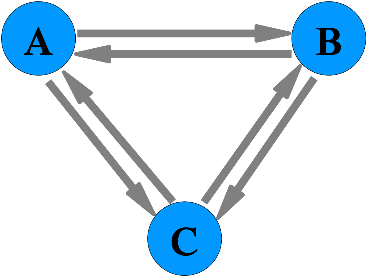
| B | C | A | A | C | B | A | B | C | ||
|---|---|---|---|---|---|---|---|---|---|---|
| 0 | 0 | 0 | 0 | 0 | 0 | 0 | 0 | 1 | ||
| 0 | 1 | 0 | 0 | 1 | 0 | 0 | 1 | 1 | ||
| 1 | 0 | 1 | 1 | 0 | 1 | 1 | 0 | 1 | ||
| 1 | 1 | 1 | 1 | 1 | 1 | 1 | 1 | 1 |

In the chaotic phase, , the distribution of transient times can be estimated from the joint probability distribution for transient times and attractor lengths derived in [32] using an annealed approximation,
| (2) | |||||
for large and . In general, depends on . It was shown in Ref. [32] that vanishes for , and approaches the value for the random map. Bastolla and Parisi also pointed out that, while the analytical expressions for the transient time distribution may not be good approximations for small , the time scale derived using the annealed approximation (see Eq. (2)) is in good agreement with their simulations for .
This last result is confirmed by our numerical simulations for various values of . Fig. 6 shows that for the random map and various indeed exhibits finite size scaling with characteristic time . For we also find a reasonable data collapse, shown in Fig. 7 using the value obtained in [32]. Yet, the quality of the data collapse continues to deteriorate as decreases to .


Fig. 8 shows the distribution of transient times along with the theoretical predictions given by Eq. (2). For the random map, the prediction is exact and the agreement between data and theory is excellent. For the theoretical predictions do not match the data for small . The theoretical curve in Eq.(2) decreases monotonically with for all . However, the actual distribution increases initially with for all considered. This increase becomes more prominent for smaller .
The number of states in the ensemble that are at a distance from an attractor is . Considering the arboreal structure of the SSN, this number corresponds to the number of states in the -th shell. An increase of for small then means that the shells become more populated with distance from an attractor. The monotonic decrease of Eq. (2) indicates that the (attractor) shell should be the most populated, which we do observe for the random map. The maxima observed in Fig. 8 for RBNs with indicate the existence of a new characteristic distance for RBNs with that does not appear in the random map.

The ratio of the sizes of consecutive shells are shown in Fig. 9. A state in the -th shell can be seen as branching from its image in the -th shell. If each basin of the SSN is viewed as a tree with the attractor at its root, Fig. 9 gives a mean branching ratio from the -th shell to the -th shell for the whole ensemble. Note that this is not the mean of the branching ratios for each attractor basin. For , Fig. 9 shows that for small the shells first grow at a rate that slows down with distance from the attractors. The growth eventually stops and the shells become smaller and smaller for increasing when it is larger than a certain value that depends on (and on ). This turn around happens when the ratio drops below unity. For the random map, Eq. (2) implies that shells should become smaller for all , albeit very slowly. This can be seen in Fig. 9 in which the random map curve almost coincides with unity. The curve crosses unity and quickly merges with the random map curve, while the and curves make a discernible dip below the line, the extent of the dip depending on . Indeed it appears that the behavior of the branching ratio for RBNs shows more variation than other values of .

Both the value of where the branching ratio is minimal and the value where increase with increasing as shown for in Fig. 10. The roughly linear increase also appears to hold for . If the growth that we find in Fig. 10 can be extrapolated to large system sizes, our results indicate the existence of a new diverging time scale for RBNs with that is unrelated to the cut-off for large arguments given by Eq. (2).
IV Results for the segment polarity network of Drosophila melanogaster
To compare our results for RBNs with a biological signaling network, we consider the segment polarity network of fruit flies [16]. This Boolean model of the gene and protein interactions involved in embryonic pattern formation in the fruit fly Drosophila melanogaster is a particularly well-documented and successful application. In particular, it reproduces many experimentally observed features, including knock out results, indicating that knowledge of the kinetic details are not necessary.
The model presented in [16] considers gene expression patterns in four adjacent cells that form a Drosophila parasegment. Each cell is modelled by a network of fifteen Boolean elements. Each element represents either an mRNA species or a protein species in the cell. The state of each element is one if the corresponding species is expressed, otherwise it is zero. Each element in a cell can interact with elements within the same cell as well as elements in the neighboring cells. All interactions are modelled by Boolean functions. Of the 15 species, the state of protein “sloppy-paired” (SLP) in each of the 4 cells is fixed to its biologically relevant value. The resulting state space contains 6 fixed point attractors.
Here we study the dynamics of only one cell, for two reasons. First, the complete network, which consists of 60 elements, is computationally untractable using exact enumeration. Second, a single cell represents the building block of the entire organism. Understanding the dynamics of a single cell is important to understand the whole network. Robust dynamics of the individual cells that form the segment has been argued to underlie the observed robustness of expression patterns of the whole segment [33].A differential equation model for individual cells based on the original work in [34] was used to show this relation between the dynamics of the individual cells and the whole segment. In the same vein, here we study the state space of the Boolean network for an individual cell. As a result, our individual cell network cannot be directly compared with the parasegment network studied in [16].
In the Boolean network model of [16], cells interact via three elements, the hedgehog mRNA (hh), the hedgehog protein (HH), and the wingless protein (WG). To reduce the model to one individual cell, we replace the values of these three elements in the cell’s neighbourhood by three new variables, hhN, HHN and WGN. Each of these three elements evolves by copying its state. Furthermore SLP also copies its own state. Therefore, the values of the states of these four elements are fixed by the initial conditions and do not evolve dynamically. Note that this ensures the existence of at least different attractors, each corresponds to a unique combination of the input elements.
The polarity network studied here contains elements in total. The connectivity, , of the nodes in the polarity network is distributed as follows: nodes have , have , have and only one node has . The mean connectivity in the network is thus . The Boolean rules (functions) of the nodes in the network are given in Table 1. The average bias, , in the network is . The internal homogeneity, which measures the average percentage of the most abundant outcome (zero or one) in each Boolean function, is .
| Node | Boolean function (input/output relation) |
|---|---|
| wg | (CIA AND SLP AND NOT CIR) |
| OR (wg AND (CIA OR SLP) AND NOT CIR) | |
| WG | wg |
| en | WGN AND NOT SLP |
| EN | en |
| hh | EN AND NOT CIR |
| HH | hh |
| ptc | CIA AND NOT EN AND NOT CIR |
| PTC | ptc OR (PTC AND NOT HHN) |
| PH | PTC AND HHN |
| SMO | NOT PTC OR HHN |
| ci | NOT EN |
| CI | ci |
| CIA | CI AND (SMO OR hhN) |
| CIR | CI AND NOT SMO AND NOT hhN |
| SLP | SLP (input) |
| hhN | hhN (input) |
| HHN | HHN (input) |
| WGN | WGN (input) |
We find that the individual cell state space has different attractors, each of which is a fixed point. The states of the 21 attractors are shown in Fig. 11. Each of columns in the figure represents an attractor. Each of rows represent the value of the Boolean state of a particular element across different attractors. The black squares depict ones while white squares depict zeros.
Fig. 11 also illustrates the clustering of attractors in configuration space. Attractors in the figure are arranged in clusters where neighboring attractors in each cluster are one bit flip away. Note that the bit flips that immediately lead to a different attractor are all flips of the relevant component. In this context, there are at least 4 relevant components in the network 22 2 Note that the existence of attractors instead of is an indication of the existence of further relevant components. For instance, one can notice that nodes wg and PTC copy themselves under certain configurations of their input elements, thus becoming relevant. However, bit flips to these elements doesn’t lead directly to another attractor.. SLP, hhN, HHN, and WGN all copy their own state at each time step, therefore each is a relevant component.
We note that the attractors in Fig. 11 capture the cell states observed in Drosophila segments. For example, none of the cells in the Drosophila segment co-express genes wg and en [35]. Lack of wg-en co-expression is also seen in the attractors in Fig. 11. Our results suggest that the observed gene expression phenotype of the segment polarity network stems from the constrained dynamics in a single cell, rather than the complex interactions between the cells. The same has been argued previously in [33] using a differential equation model for a single cell. The biological significance of these results and their impact on gene expression robustness will be expounded in a future publication [36].

Avalanches and transients for the segment polarity network are defined in the same way as for RBNs — see section II. Fig. 12 shows the distributions of avalanche and transient times for the segment polarity network in Table 1. As for RBNs (see, for example, Fig. 4) there are more short avalanches than short transients indicating that attractors cluster in configuration space. This holds for the specific avalanches that return to the same attractor as well as those that go to a different attractor. Interestingly, in the latter case there is a significant probability that an avalanche will immediately reach another attractor — similar to the case of RBNs with .

The qualitative similarities between RBNs and the Drosophila polarity network are also demonstrated in Fig. 13 where the distributions for RBNs with are shown for comparison. The large scatter, due to the fact that we are examining only one network rather than an ensemble, prevents any precise quantitative comparison between the segment polarity network and RBNs. It is interesting to note, though, that the distributions of avalanche durations for the polarity network have a tendency to be more similar to RBNs with at small values of than any other .

V Conclusions
We have studied avalanches on Random Boolean Networks and on the segment polarity network of Drosophila by performing bit-flip perturbation to attractor states and waiting for the dynamics to relax back to an attractor. In both cases (assuming for RBNs), there are more avalanches of short duration than what would be expected based on the distribution of transients times. This indicates that attractors tend to cluster in configuration space.
For the random map, which corresponds to RBNs with , the distribution of avalanche durations, , is identical to the distribution of transient times, . As analytically confirmed, the distribution tends to form a plateau with a sharp finite-size cut-off. For , deviations from this behavior occur for small arguments such that the plateau eventually disappears as . In particular, the deviations for small arguments are different for and . The critical case exhibits different behavior. In this case, both distributions are broad and neither the plateau nor the cut-off are observed. Their scale-free appearance suggests that the distribution of avalanche durations as well as the distribution of transient times can be used as possibly distinct indicators for the criticality in discrete, deterministic dynamical systems. Indeed we find that the avalanche durations for the Drosophila segment polarity network follows more closely the behavior (compared to other values of ) while no clear statement can be made about transient times for the Drosophila network we analyzed.
The similarity of and for large arguments and indicates that initial avalanche states that are far away from an attractor are independent of the states on the attractors (this is true for all arguments in the case of the random map). The arboreal structure of the SSN, the mean branching of which was presented in Fig 9, also seems to become more similar to that of the random map for large .
However, the branching ratio is a non-monotonic function of , crossing unity and then passing through a minimum before it starts to resemble the random-map behavior for larger . Along with our results for the differences between and for small arguments, this indicates that while states lying closer to the attractors in the SSN are correlated with the attractor states, this correlation decays as one moves away from the attractors on the SSN. The time scale at which this correlation in the arboreal structure of the SSN decays, or in which the growth rate of the tree structure in state space changes from increasing to decreasing may be a new characteristic scale for RBNs. It appears to diverge roughly linearly with the system size . This time scale does not appear in the random map and is not related to that previously studied in [32], which grows exponentially with the system size . Beyond that scale, the SSN of an RBN in the non-frozen regime may correspond to a random map, while the regions around attractors are distorted by their presence.
Acknowledgements.
We would like to thank Peter Grassberger for useful comments. This work was partially supported by NSERC.References
- [1] S. Kauffman, J. Theor. Biol. 22, 437 (1969).
- [2] B. Drossel, eprint arXiv: 0706.3351 (2007).
- [3] S. Bornholdt, Science 310, 449 (2005).
- [4] M. Aldana, S. Coppersmith, and L. Kadanoff, In Perspectives and Problems in Nonlinear Science (Springer,New York, 2003), pp. 23–89.
- [5] L. Wang, E. Pichler, and J. Ross, Proc. Natl. Acad. Sci. U. S. A. 87, 9467 (1990).
- [6] J. Lynch, Proceedings of the sixth international seminar on Random graphs and probabilistic methods in combinatorics and computer science table of contents pp. 239–260 (1995).
- [7] M. Paczuski, K. Bassler, and Á. Corral, Phys. Rev. Lett. 84, 3185 (2000).
- [8] C. Baillie and D. Johnston, Phys. Lett. B 326, 51 (1994).
- [9] B. Derrida and H. Flyvbjerg, J. Physique 48, 971 (1987).
- [10] B. Derrida and Y. Pomeau, Europhys. Lett. 1, 45 (1986).
- [11] S. Kauffman, The Origins of Order (Oxford Univ. Press, 1993).
- [12] P. Bak, How Nature Works (Copernicus New York, NY, USA, 1996).
- [13] P. Bak, C. Tang, and K. Wiesenfeld, Phys. Rev. Lett. 59, 381 (1987).
- [14] P. Bak, K. Chen, and M. Creutz, Nature 342, 780 (1989).
- [15] N. Packard, Adaptation Toward the Edge of Chaos. (University of Illinois at Urbana-Champaign, Center for Complex Systems Research, 1988).
- [16] R. Albert and H. Othmer, J. Theor. Biol. 223, 1 (2003).
- [17] F. Greil, B. Drossel, and J. Sattler, New J. Phys. 9, 373 (2007).
- [18] B. Drossel, Phys. Rev. E 72, 016110 (2005).
- [19] B. Samuelsson and C. Troein, Phys. Rev. Lett. 90, 98701 (2003).
- [20] A. Goldbeter, Nature 420, 238 (2002).
- [21] J. J. Tyson, K. C. Chen, and B. Novak, Curr. Opin. Cell Biol. 15, 221 (2003).
- [22] H. Flyvbjerg and N. Kjaer, J. Phys. A: Math. Gen. 21, 1695 (1988).
- [23] B. Drossel, T. Mihaljev, and F. Greil, Phys. Rev. Lett. 94, 88701 (2005).
- [24] A. Shreim, A. Berdahl, V. Sood, P. Grassberger, and M. Paczuski, New J. Phys. 10, 013028 (2008).
- [25] A. Bhattacharjya and S. Liang, Phys. Rev. Lett. 77, 1644 (1996).
- [26] C. Fretter and B. Drossel, eprint arXiv: 0801.3784 (2008).
- [27] A. Shreim, P. Grassberger, W. Nadler, B. Samuelsson, J. Socolar, and M. Paczuski, Phys. Rev. Lett. 98, 198701 (2007).
- [28] E. R. Berlekamp, J. H. Conway, and R. K. Guy, Winning Ways for Your Mathematical Plays Vol. 2 (Academic, 1982).
- [29] A. Berdahl, V. Sood, A. Shreim, M. Paczuski, and J. Davidsen, in preparation (2008).
- [30] V. Kaufman and B. Drossel, New J. Phys. 8, 228 (2006).
- [31] J. Socolar and S. Kauffman, Phys. Rev. Lett. 90, 68702 (2003).
- [32] U. Bastolla and G. Parisi, Physica D 98, 1 (1996).
- [33] N. Ingolia, PLoS Biol 2, e123 (2004).
- [34] G. von Dassow, E. Meir, E. Munro, and G. Odell, Nature 406, 188 (2000).
- [35] B. Sanson, EMBO Reports 2, 1083 (2001).
- [36] V. Sood, A. Berdahl, A. Shreim, and M. Paczuski, Hierarchy of robustness in interacting cells (2008), in preparation.