SLAC-PUB-13222
Identification of the Origin of Monojet Signatures at the LHC ** * Work supported in part by the Department of Energy, Contract DE-AC02-76SF00515†† † e-mail: rizzo@slac.stanford.edu
Thomas G. Rizzo
Stanford Linear Accelerator Center, 2575 Sand Hill Rd., Menlo Park, CA, 94025
Several new physics scenarios can lead to monojet signatures at the LHC. If such events are observed above the Standard Model background it will be important to identify their origin. In this paper we compare and contrast these signatures as produced in two very different pictures: vector or scalar unparticle production in the scale-invariant/conformal regime and graviton emission in the Arkani-Hamed, Dimopoulos and Dvali extra-dimensional model. We demonstrate that these two scenarios can be distinguished at the LHC for a reasonable range of model parameters through the shape of their respective monojet and/or missing distributions.
1 Introduction and Background
The LHC will turn on during 2008 and it is generally expected that new physics beyond the Standard Model(SM) will be discovered at some point thereafter once significant luminosity is accumulated and the the two detectors are sufficiently well-understood. What new physics signatures will be observed and how will they be grounded within a specific theoretical framework? Clearly once the new physics is found, our primary goal will be to uncover its origin and to identify the underlying model which generates it. This can sometimes be confusing as in many cases several kinds of new physics can lead to quite similar signatures at colliders. Supersymmetry[1] and Universal Extra Dimensions[2] provide us with one well-known example of this possible model confusion which has been much discussed in the recent literature[3]. The ability of the LHC to differentiate models with similar signatures may become the the most important issue once new physics is discovered.
In this paper we will consider another example of this kind of potential confusion which may arise at the LHC between two very different scenarios: graviton emission in the extra-dimensional model of Arkani-Hamed, Dimopoulos and Dvali(ADD)[4] and the production of scalar/vector unparticles in the model of Georgi[5] in the scale-invariant/conformal regime[6] where the unparticle can be treated as both ‘massless’ and stable. Here, by a ‘massless’ unparticle we will mean one that has a null threshold mass parameter, i.e., , which determines the minimum allowed value of its possible squared 4-momentum[6], i.e., . (Recall that for unparticles the value of actually takes on a continuous range which is integrated over to obtain observable cross sections.) Both of these new physics models can lead to a monojet signal, i.e., a single jet plus missing (MET) with balancing transverse momenta, at the LHC. In the ADD case, this scenario has been studied in some detail in the classic work by Vacavant and Hinchliffe[7] within the ATLAS[8] setting, which we will use as a guide for the present analysis.‡‡ ‡ CMS[9] has also performed a more recent but comparable analysis in the single photon channel. Assuming that monojet signals above the SM backgrounds are indeed observed at the LHC we will demonstrate that the shapes of the corresponding excess jet and/or missing distributions are qualitatively quite distinctive in these two cases. This will allow these two classes of models to be distinguished at the LHC for a range of parameters provided that sufficient integrated luminosity is available.
As emphasized by Vacavant and Hinchliffe[7], observing an excess in the monojet channel relies on our thorough understanding of the SM background. At low , this background can be dominated by QCD/jet energy mis-measurements. However, at high it is largely dominated by production followed by the decay . Fortunately, in practice, it appears that neither ATLAS nor CMS[10] will need to rely solely on Monte Carlo estimates to fully understand this MET plus jet(s) background. At high one can instead employ the ‘standard candle’ approach where one makes use of the same production channel but now with the decaying leptonically, i.e., . These easily measured rates can then be corrected for differences in the branching fractions as well as for acceptances and efficiencies to obtain the -induced SM monojet background[11] directly from data. Other sources of background, such as production with with the two jets coalescing due to the boost, can also be handled in a similar fashion though we expect them to be about an order of magnitude smaller in rate. In the analysis presented below we will assume that this procedure works so that these backgrounds will eventually be well understood in the very high region above 500 GeV, corresponding to an TeV upon which we will concentrate. We will not include in the present analysis possible additional information that may be obtainable from the lower region where the jet energy mis-measurements can be a potentially large source of SM backgrounds. The resulting SM background estimates that we obtain and will employ below are found to be essentially the same as, though perhaps larger than, those found by Vacavant and Hinchliffe[7]. Of course the background in this analysis is not the issue at hand. Our goal is to inquire whether or not the ADD and unparticle predictions can be distinguished provided a well-defined signal over background is already clearly observed.
Our procedure is rather straightforward: First, we will demonstrate that the overall shape of the normalized monojet distribution predicted by the ADD model is essentially independent of the number of extra dimensions in the relevant parameter range. Next we will show that the predictions for the corresponding normalized monojet spectra produced by either scalar and vector unparticles lie in a rather narrow band. By comparing these two sets of distributions it will then become clear that for sufficiently high integrated luminosities, , these two predictions will be easily isolated from one another in space so that we can distinguish these two classes of models at the LHC by using the data collected above GeV.
2 Analysis
Let us begin by considering the monojet signal[12] in the ADD model which arises from graviton Kaluza-Klein tower () emission in the following processes: and . The expressions for these parton-level cross sections are given in full detail in Ref.[12]. In the original ADD scenario, the resulting cross section expressions depend upon only 2 parameters: the number of extra dimensions, , and the value of the -dimensional Planck scale, ; these subprocess level cross sections are observed to scale as . Since the ADD model is only an effective theory below a cut off scale , in performing the integrations necessary to obtain the relevant LHC cross sections it is unclear how to treat the kinematic region where the partonic center of mass energy, , is in excess of unless one has a more fundamental theory to rely upon. There are two common ways that have been used to address this issue discussed in the literature[7, 12]. First, we could simply ignore this problem and perform the necessary integration; a second possibility is to make a hard truncation in the integration at , both of which are unrealistic. The former choice will, of course, lead to a larger event rate but one finds that these two approaches yield qualitatively similar but quantitatively different numerical results.
In performing our analysis, we will instead follow a better approach and make use of a realistic underlying fundamental theory based on non-perturbative General Relativity in extra dimensions. This approach leads directly to non-Gaussian fixed-points in the gravitational coupling that predicts the existence of a gravitational form factor[13] which naturally controls the large part of the cross section, extending the range of validity of the partonic cross section above and maintains unitarity at high energies. It is important to note that this is not an ad-hoc use of an arbitrary form factor as the underlying dynamics dictates the form factor structure and power behavior as well as the form factor scale itself up to a factor close to unity. For numerical purposes we will use a fixed form factor scale of TeV in this analysis. One finds, however, that varying this particular choice will make little numerical difference in the qualitative nature of the results presented below, and as an explicit examination reveals, since the form factor only leads to modifications in the extreme high end of the various distributions where there are very limited statistics as we will see.


Since our goal is to differentiate monojet signals arising in different models by the shapes of their jet distributions, it is instructive to first compare the ADD model ‘with itself’, i.e., to compare the ADD predictions for different values of while simultaneously varying the value of (as a function of ) so that the models all predict the same cross section at some fixed value of the jet . This allows us to directly compare the predicted shape for the signal monojet spectrum for each value of without having to worry about the overall normalization of the spectrum. Note that in all cases the subprocess cross sections for graviton emission are seen to grow rapidly with and so can naturally lead to large event excesses at high . As an example, let us assume a reference value for the monojet cross section corresponding to the choice of with TeV. For all larger values of we will then adjust the associated value of such that identical cross sections are obtained when evaluated at a jet energy of GeV. Note that there is nothing particularly special about this choice of value other than it allows us to have a reasonable signal-to-background ratio for all values of for the integrated luminosities that we will assume in our analysis. Other choices for this cross-over point in the ADD case would yield qualitatively similar results since we are only probing the various shapes of the distributions here. We next determine the resulting LHC monojet event rates for each case as a function of jet while simultaneously demanding that the monojet be more or less central in rapidity, i.e., , as assumed by Vacavant and Hinchliffe[7]; to be specific, we employ the CTEQ6.6M PDFs[14] throughout and will assume a fixed integrated luminosity of 100 . In a similar manner, we can also ask for the cumulative number of events above a minimum cut on the jet which probes a somewhat different aspect of the jet spectrum. As we will see, the additional statistics in this distribution will allow for an improved separation of models.


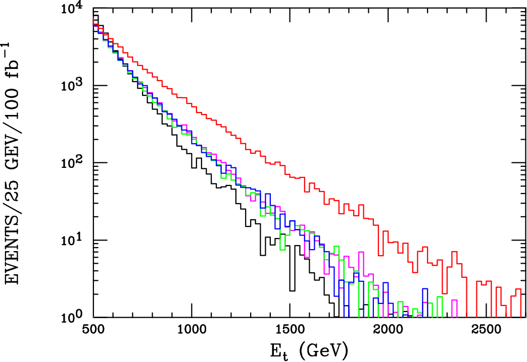
The results of this analysis together with an estimate of the SM induced backgrounds are shown in Fig. 1 for assuming jet ’s larger than 500 GeV. Here we see that while the ADD model for the chosen set of parameter ranges clearly produces a significant signal above the SM background it is very difficult to determine the value of itself since all of the predicted distributions lie rather close to one another§§ § The results for are seen to lie slightly below the others so that this case may be confidently distinguished from the others at somewhat higher integrated luminosities. It is important to note, however, that the predictions for larger values of lead to slightly harder distributions.. This is seen to be an even stronger conclusion for the case of the distributions. This reproduces the well-known result[7] that at the LHC it is essentially impossible, or at least extremely difficult, to determine both the values of and simultaneously from the observation of a monojet excess at a fixed value of . However, for our purposes, this is a positive result since our goal is to distinguish the set of all ADD predictions from those of other models, specifically, those arising from unparticles. The ADD prediction for the shape of these and distributions are thus found not to be very sensitive to the specific value of , especially when . Note that if the value of GeV, chosen as the cross-over point where the various ADD predictions yield the same cross section, was taken to be somewhat larger then any determination of the value of would be only be made more difficult since the divergences in the observed spectra would be reduced. Lowering the cross-over point would increase the lever arm somewhat but, as we can easily see from this figure, would at most only be useful in separating the case from the other choices for .


In order the compare the standard approaches to the large problem in ADD and what we obtain here, a direct comparison for the case of is made as described in Fig. 2. Here we see that the predictions of form-factor analysis lies fairly close to those obtained by integration over the full kinematic range while those with a hard cut off are somewhat softer at the very high/low statistics end as would be expected. In all cases the shape/slope of this distribution is seen to be almost identical for an jet cut below TeV.
When considering the predictions of the unparticle model, with which we wish to compare the ADD scenario, the parameter space is somewhat more varied and there are many possibilities. Here, to be specific, we will consider the case of ‘massless’ unparticles, as described above, which are assumed to be either scalar (spin-0), , or vector (spin-1), , and in either case are sufficiently stable so that they can lead to a collider missing signature. However, we have checked that by adding a small unparticle threshold mass, GeV, so that , we will not significantly alter the numerical results presented below as long as the relative stability of the unparticle on collider scales is also maintained. This is clear since for these processes small threshold masses for the unparticles will only result in a small reduction in the size of the relevant phase space which is of order . Having made these particular choices, several other parameter options still can remain. If we take the simplest possibility and assume that the unparticle couples as a SM gauge singlet to only one operator constructed of only single type of SM field, then the resulting interaction will depend upon only an overall scale, , as well as the value of the effective unparticle anomalous dimension, , which is restricted to lie in the range . If, however, the unparticle is allowed to couple to several different SM operators, then the relative strengths of these interactions, , can also become quite relevant. Here, to be specific, we will assume that the spin-0 unparticles couple to the relevant SM fields via
| (1) |
for all quark fields and where is the gluon field strength tensor; we will consider the two cases below as representative examples. We will further assume that the spin-1 unparticles couple only to the SM quarks via
| (2) |
also in a universal manner. The parton-level cross sections for the relevant processes , and can be found in Ref.[15]. Correspondingly, we find that the (reduced) spin and color-averaged squared matrix elements for the remaining processes of interest are given, in a slightly modified version of the notation of Ref.[15], by
| (3) | |||||
where is the unparticle invariant mass, as defined above, which is integrated over to obtain a final cross section result. A similar expression is found to hold in the case of the initial state. The corresponding differential cross sections are then given by
| (4) |
where is the usual subprocess-level Mandelstam variable and is the familiar unparticle numerical phase space factor as given by Georgi[5]. It is interesting to note that the scaling behavior of the unparticle cross sections for both the unparticle vectors and scalars is such that they will lead to essentially the same dependence as the SM background in the limit when . This is not surprising since in that limit the unparticles behave in a manner similar to the more conventional SM boson fields. In keeping with the ADD distribution shape analysis above, we will in all cases adjust the value of the scale so that the unparticle monojet cross section at GeV is the same as that for the ADD model with TeV with at the same . In order to do this it is obvious that different values of will need to be chosen as both and are varied for both the scalar and vector unparticle cases independently.


Figs. 3, 4 and 5 show the results analogous to Fig. 1 for the vector unparticle as well as the scalar unparticle cases with , respectively. Several things are immediately obvious from these figures. First, as expected, the overall shape of the unparticle and spectra becomes stiffer as the value of is increased. This is not too surprising as the leading subprocess cross sections are observed to scale as relative to the SM background. Secondly, the distributions we obtain for both the scalar and vector particles are, for the same value of , essentially of the same shape. Again, this is not surprising as these two case differ only in the tensor structure of the unparticle interaction. The and scalar interactions are slightly different due to the additional unparticle coupling to the gluon. While this operator is suppressed by an additional power of , the initial state luminosity at relatively low is very large and somewhat offsets this suppression. All in all, the predictions for the monojet spectra of these representative unparticle models are found to lie in a somewhat narrow band which is observed to be harder at high and than is the SM background.

Up to now we have found that both the ADD predictions for the monojet and spectra and those from unparticles separately lie in rather restricted ranges. How do these ranges compare? Since the hardest spectrum in the unparticle model is obtained for large and the softest spectrum for ADD occurs when it is most instructive to compare these specific two cases. Any other pair of spectra will clearly lie further apart in space and so will be more easily distinguished. Fig. 6 shows a representative set of comparisons of these two cases taking the above observations into account. Here we see that the three sample unparticle model predictions are relatively clustered together and lie in between those for the ADD scenario and the SM background. While the unparticle predictions themselves are difficult to distinguish it is clear that they are all easily differentiable from those of the ADD model. It is clear that a very large amount of jet energy smearing would be necessary to make these two predicted regions appear to overlap to any extent. These results demonstrate that with enough statistics the shapes of the excess monojet distributions arising from these two classes of models can be distinguished at the LHC provided that they are visible above the SM background. We would, however, hope that a more detailed study by ATLAS/CMS using a full detector simulation will be performed to verify these results.
3 Discussion and Conclusions
In this paper we have explored the capability of the high luminosity LHC to differentiate two sets of new physics models that can lead to visible missing /monojet signatures. The relevant tools for model discrimination are the shapes of the resulting monojet and distributions themselves. First, we demonstrated that () the predictions of the ADD for the monojet distributions form a very narrow band for and, () Similarly, the corresponding predictions in the case of vector or scalar unparticles also so lie in a different but not so narrow band. Second, we showed that these two bands are seen not to overlap when integrated luminosities of order are available implying that these two classes of models which induce the monojet signal can be distinguished at the LHC.
References
- [1] For a phenomenological introduction to SUSY, see H. Baer and X. Tata, Weak scale supersymmetry: From superfields to scattering events, Cambridge, UK: Univ. Pr. (2006) 537 p; M. Drees, R. Godbole and P. Roy, Theory and phenomenology of sparticles: An account of four-dimensional N=1 supersymmetry in high energy physics, Hackensack, USA: World Scientific (2004) 555 p.
- [2] T. Appelquist, H. C. Cheng and B. A. Dobrescu, Phys. Rev. D 64, 035002 (2001) [arXiv:hep-ph/0012100].
- [3] There has been much work on this subject; see for example, A. Datta, K. Kong and K. T. Matchev, Phys. Rev. D 72, 096006 (2005) [Erratum-ibid. D 72, 119901 (2005)] [arXiv:hep-ph/0509246]; C. Athanasiou, C. G. Lester, J. M. Smillie and B. R. Webber, JHEP 0608, 055 (2006) [arXiv:hep-ph/0605286]; L. T. Wang and I. Yavin, JHEP 0704, 032 (2007) [arXiv:hep-ph/0605296]; J. M. Smillie, Eur. Phys. J. C 51, 933 (2007) [arXiv:hep-ph/0609296]; S. Y. Choi, K. Hagiwara, H. U. Martyn, K. Mawatari and P. M. Zerwas, Eur. Phys. J. C 51, 753 (2007) [arXiv:hep-ph/0612301]; C. Kilic, L. T. Wang and I. Yavin, JHEP 0705, 052 (2007) [arXiv:hep-ph/0703085]; C. Csaki, J. Heinonen and M. Perelstein, JHEP 0710, 107 (2007) [arXiv:0707.0014 [hep-ph]]; L. T. Wang and I. Yavin, arXiv:0802.2726 [hep-ph].
- [4] N. Arkani-Hamed, S. Dimopoulos and G. R. Dvali, Phys. Lett. B 429, 263 (1998) [arXiv:hep-ph/9803315].
- [5] H. Georgi, Phys. Lett. B 650, 275 (2007) [arXiv:0704.2457 [hep-ph]] and H. Georgi, Phys. Rev. Lett. 98, 221601 (2007) [arXiv:hep-ph/0703260].
- [6] See for example P. J. Fox, A. Rajaraman and Y. Shirman, Phys. Rev. D 76, 075004 (2007) [arXiv:0705.3092 [hep-ph]]; A. Delgado, J. R. Espinosa and M. Quiros, JHEP 0710, 094 (2007) [arXiv:0707.4309 [hep-ph]]; M. J. Strassler, arXiv:0801.0629 [hep-ph]; V. Barger, Y. Gao, W. Y. Keung, D. Marfatia and V. N. Senoguz, Phys. Lett. B 661, 276 (2008) [arXiv:0801.3771 [hep-ph]].
- [7] L. Vacavant and I. Hinchliffe, J. Phys. G 27, 1839 (2001).
- [8] ATLAS Detector and Physics Performance Technical Design Report, http://atlas.web.cern.ch/Atlas/GROUPS/PHYSICS/TDR/access.html.
- [9] CMS Physics Technical Design Report, https://cmsdoc.cern.ch/cms/cpt/tdr/ and G. L. Bayatian et al. [CMS Collaboration], J. Phys. G 34, 995 (2007).
- [10] For a discussion, see M. Spiropulu, arXiv:0801.0318 [hep-ex]; C. Buttar et al., arXiv:0803.0678 [hep-ph]; M. Tytgat, arXiv:0710.1013 [hep-ex]; A. Tricomi, talk given at HEP2007, Manchester, England, 19-25 July 2007; G.Polesello and V. Zhuravlov, talks give at the ‘Physics at the Terascale’ Workshop, DESY, 03-05 December 2007; R. Cavanaugh, talk given at the 2008 Aspen Winter Conference, 13-19 January 2008; S. Tsuno, talk given at Moriond Electroweak 2008, La Thuile, Italy, 01-08 March 2008; A. De Roeck, talk given at Physics of the Large Hadron Collider Workshop, Kavli Institute, UCSB, 01 April 2008.
- [11] This method has already been used successfully at the Tevatron: A. Abulencia et al. [CDF Collaboration], Phys. Rev. Lett. 97, 171802 (2006) [arXiv:hep-ex/0605101]; V. M. Abazov et al. [D0 Collaboration], Phys. Rev. Lett. 90, 251802 (2003) [arXiv:hep-ex/0302014].
- [12] G. F. Giudice, R. Rattazzi and J. D. Wells, Nucl. Phys. B 544, 3 (1999) [arXiv:hep-ph/9811291].
- [13] For a discussion, see J. Hewett and T. Rizzo, JHEP 0712, 009 (2007) [arXiv:0707.3182 [hep-ph]]; and also D. F. Litim and T. Plehn, Phys. Rev. Lett. 100, 131301 (2008) [arXiv:0707.3983 [hep-ph]], and references therein.
- [14] P. M. Nadolsky et al., arXiv:0802.0007 [hep-ph].
- [15] K. Cheung, W. Y. Keung and T. C. Yuan, Phys. Rev. D 76, 055003 (2007) [arXiv:0706.3155 [hep-ph]] and Phys. Rev. Lett. 99, 051803 (2007) [arXiv:0704.2588 [hep-ph]].