Information, Energy and Density for Ad Hoc Sensor Networks over Correlated Random Fields: Large Deviations Analysis

Large deviations analysis of Gauss-Markov processes in Gaussian noise has been considered previously. (See [2] and references therein.) However, most work in this area considers only one-dimensional (1-D) signals or time series. A closed-form expression for the asymptotic KLI rate was obtained and its properties were investigated for 1-D hidden Gauss-Markov random processes [2]. Large deviations analyses were used to examine the issues of optimal sensor density and optimal sampling in a 1-D signal model in [3] and [4]. For a 2-D setting, an error exponent was obtained for the detection of 2-D GMRFs in [5], where the sensors are located randomly and the Markov graph is based on the nearest neighbor dependency enabling a loop-free graph. In this work, however, measurement noise was not considered. Our work here focuses on the analysis of the fundamental behavior of 2-D sensor networks deployed for statistical inference via new large deviations results for 2-D hidden GMRFs, which enable us to investigate the impact of field correlation and measurement signal-to-noise ratio (SNR) on the information.

To investigate the properties of the asymptotic KLI and MI rates as functions of field correlation and SNR, we further consider the symmetric first order conditional autoregression (SFCAR), defined by the conditions

	$\displaystyle{\mathbb{E}}\{X_{ij}|{\bf X}_{-ij}\}$	$\displaystyle=$	$\displaystyle\frac{\lambda}{\kappa}(X_{i+1,j}+X_{i-1,j}+X_{i,j+1}+X_{i,j-1}),$
	$\displaystyle\mbox{Prec}\{X_{ij}|{\bf X}_{-ij}\}$	$\displaystyle=$	$\displaystyle\kappa>0,$

where $0\leq\lambda\leq\frac{\kappa}{4}$. (This is a sufficient condition to satisfy (7) - (8).) Here, $\theta_{00}=\kappa$ and $\theta_{1,0}=\theta_{-1,0}=\theta_{0,1}=\theta_{0,-1}=-\lambda$. In the SFCAR model, the correlation is symmetric for each set of four neighboring sensor nodes. The SFCAR model is a simple but meaningful extension of the 1-D autoregression (AR) model which has the conditional causal dependency only on the previous sample. Here in the 2-D case we have conditional dependence on four neighboring nodes in the four (planar) directions, capturing 2-D correlation structure. The spectrum of the SFCAR signal is given by

$$f(\omega_{1},\omega_{2})=\frac{1}{4\pi^{2}\kappa(1-2\zeta\cos\omega_{1}-2\zeta\cos\omega_{2})},$$

(12)

where the edge dependence factor $\zeta$ is defined as

$$\zeta\stackrel{{\scriptstyle\Delta}}{{=}}\frac{\lambda}{\kappa},~~~~0\leq\zeta\leq 1/4.$$

(13)

Here, $\zeta=0$ corresponds to the i.i.d. case whereas $\zeta=1/4$ corresponds to the perfectly correlated case. Therefore, the correlation strength can be captured in this single quantity $\zeta$ for SFCAR signals. The power of the SFCAR is obtained using the inverse Fourier transform via the relationship (3), and is given by $P_{s}=\gamma_{00}=\frac{2K(4\zeta)}{\pi\kappa},~\left(0\leq\zeta\leq\frac{1}{4}\right)$, where $K(\cdot)$ is the complete elliptic integral of the first kind [9]. The SNR is given by $\mbox{SNR}=\frac{P_{s}}{\sigma^{2}}=\frac{2K(4\zeta)}{\pi\kappa\sigma^{2}}$. Using (10) and the SNR, we obtain the asymptotic KLI and MI rates for the SFCAR signal, given in the following corollary to Theorem 1, also from [7].

Note that the SNR and correlation are separated in (14)-(15), which enables us to investigate the effects of each term separately.

First, it is readily seen from Corollary 1 that $\mbox{$\mathscr{K}$}_{s}$ and $I_{s}$ are continuously differentiable $C^{1}$ functions of the edge dependence factor $\zeta$ ($0\leq\zeta\leq 1/4$) for a given SNR since $f:x\rightarrow K(x)$ is a continuously differentiable $C^{\infty}$ function for $0\leq x<1$ [10]. The values of ${\cal K}_{s}$ at the extreme correlations are given by noting that $K(0)=\frac{\pi}{2}\ \ {\rm and}\ \ K(1)=\infty$. Therefore, in the i.i.d. case ($\zeta=0$), the corollary reduces to Stein’s lemma as expected, and $\mbox{$\mathscr{K}$}_{s}$ is given by

$$\mbox{$\mathscr{K}$}_{s}|_{\zeta=0}=\frac{1}{2}\log(1+\mbox{SNR})+\frac{1}{2(1+\mbox{SNR})}-\frac{1}{2}=D({\cal N}(0,1)||{\cal N}(0,1+\mbox{SNR})).$$

In the i.i.d. case, the asymptotic MI rate is given by the well known formula, $I_{s}|_{\zeta=0}=\frac{1}{2}\log(1+\mbox{SNR})$. For the perfectly correlated case ($\zeta=1/4$), on the other hand, $\mbox{$\mathscr{K}$}_{s}=0$ and $I_{s}=0$. (In this case as well as in the i.i.d. case, the two-dimensionality is irrelevant.) The limiting behavior of the asymptotic information rates is given by Taylor’s theorem. Due to the continuous differentiability, we have

	$\displaystyle\mbox{$\mathscr{K}$}_{s}(\zeta)$	$\displaystyle=$	$\displaystyle c_{1}\cdot(1/4-\zeta)+o(|1/4-\zeta|),$		(16)
	$\displaystyle I_{s}(\zeta)$	$\displaystyle=$	$\displaystyle c_{1}^{\prime}\cdot(1/4-\zeta)+o(|1/4-\zeta|),$		(17)

for some constants $c_{1}$ and $c_{1}^{\prime}$, as $\zeta\rightarrow 1/4$. Similarly, we also have the linear limiting behavior for $\mbox{$\mathscr{K}$}_{s}$ and $I_{s}$ in a neighborhood of $\zeta=0$ with non-zero limit values, as $\zeta\rightarrow 0$. That is,

	$\displaystyle\mbox{$\mathscr{K}$}_{s}(\zeta)$	$\displaystyle=$	$\displaystyle\mbox{$\mathscr{K}$}_{s}(0)+c_{2}\zeta+o(\zeta),$		(18)
	$\displaystyle I_{s}(\zeta)$	$\displaystyle=$	$\displaystyle I_{s}(0)+c_{2}^{\prime}\zeta+o(\zeta),$		(19)

for some $c_{2}$ and $c_{2}^{\prime}$, as $\zeta\rightarrow 0$. For intermediate values of correlation, it is seen that at high SNR $\mbox{$\mathscr{K}$}_{s}$ is monotonically decreasing as $\zeta$ increases. At low SNR, on the other hand, correlation is beneficial to the performance.

With regard to $\mbox{$\mathscr{K}$}_{s}$ and $I_{s}$ as functions of SNR, the behavior of $\mbox{$\mathscr{K}$}_{s}$ is given by the following theorem.

Proof: In [8].

Note that the limiting behavior as $\mbox{SNR}\rightarrow 0$ is different for $\mbox{$\mathscr{K}$}_{s}$ and $I_{s}$; $\mbox{$\mathscr{K}$}_{s}$ decays to zero quadratically while $I_{s}$ diminishes linearly.

The actual physical correlation for the SFCAR model is given by solving the corresponding continuous-index 2-D stochastic differential equation (the stochastic Laplace equation)^†† † Note that the solution of (20) is circularly symmetric, i.e., it depends only on $r=\sqrt{x^{2}+y^{2}}$, and samples of the solution $X(x,y)$ of (20) on lattice ${\cal I}_{n}$ do not necessarily form a discrete-index SFCAR GMRF. However, (20) is still the continuous-index counterpart of the SFCAR model, and we use its correlation function for the SFCAR model. [11]

$$\left[\left(\frac{\partial}{\partial x}\right)^{2}+\left(\frac{\partial}{\partial y}\right)^{2}-\alpha^{2}\right]X(x,y)=u(x,y),$$

(20)

where $u(x,y)$ is the 2-D white zero-mean Gaussian perturbation and $\alpha>0$ is the diffusion rate. By solving the SDE, the edge correlation factor $\rho$ is given, as a function of the sensor spacing $d_{n}$, by [11]

$$\rho\stackrel{{\scriptstyle\Delta}}{{=}}\frac{\gamma_{01}}{\gamma_{00}}=\frac{\gamma_{10}}{\gamma_{00}}=f(d_{n})=\alpha d_{n}K_{1}(\alpha d_{n}),$$

(21)

where $K_{1}(\cdot)$ is the modified Bessel function of the second kind whose asymptotic behavior is given by

$$\left\{\begin{array}[]{cccl}K_{1}(x)&\rightarrow&\sqrt{\frac{\pi}{2x}}e^{-x}&\mbox{as}~x\rightarrow\infty,\\ K_{1}(x)&\rightarrow&1/x&\mbox{as}~x\rightarrow 0.\\ \end{array}\right.$$

(22)

The correlation function (21) can be regarded as the representative correlation in 2-D, similar to the exponential correlation function $e^{-Ad_{n}}$ in 1-D. Both functions decrease monotonically w.r.t. $d_{n}$. However, the 2-D correlation function is flat at $d_{n}=0$ [11]. Further, we have a continuous and differentiable mapping $g:\rho\rightarrow\zeta$ from the edge correlation factor $\rho$ to the edge dependence factor $\zeta$, given by [8]

$$\rho=\frac{(2/\pi)K(4\zeta)-1}{4(2/\pi)\zeta K(4\zeta)}=:g^{-1}(\zeta),$$

(23)

which maps zero and one to zero and 1/4, respectively. Thus, we have $\zeta=g(f(d_{n})),$ and for given physical parameters (with a slight abuse of notation),

$$\mbox{$\mathscr{K}$}_{s}(\mbox{SNR},\zeta)=\mbox{$\mathscr{K}$}_{s}(\mbox{SNR},g(f(d_{n})))=\mbox{$\mathscr{K}$}_{s}(\mbox{SNR},d_{n}).$$

(And, similarly for $I_{s}$.) We will use the arguments SNR and $\zeta$ for $\mbox{$\mathscr{K}$}_{s}$ and $I_{s}$ properly if necessary.

In the following, we summarize the assumptions for the planar ad hoc sensor network that we consider.

• (A.1)

  $n^{2}$ sensors are located on the grid ${\cal I}_{n}=[0:1:n-1]^{2}$ with spacing $d_{n}$, as shown in Fig. 1, and a fusion center is located at the center $(\lfloor n/2\rfloor,\lfloor n/2\rfloor)$.

• (A.2)

  The observations $\{Y_{ij}\}$ at sensor nodes form a 2-D hidden (discrete-index) SFCAR Gauss-Markov random field on the lattice for each $d_{n}>0$, and the edge dependence factor is given by (21) and (23).

• (A.3)

  The fusion center gathers the measurement from all nodes using the minimum hop routing. Note that the links in Fig. 1 are not only the Markov dependence edges but also the routing links. The minimum hop routing requires a hop count of $|i-\lfloor n/2\rfloor|+|j-\lfloor n/2\rfloor|$ to deliver $Y_{ij}$ to the fusion center.

• (A.4)

  The communication energy per link $E_{c}(d_{n})=E_{0}d_{n}^{\nu}$, where $\nu\geq 2$ is the propagation loss factor in wireless channel.

• (A.5)

  Sensing requires energy, and the sensing energy per node is denoted by $E_{s}$. Moreover, we assume that the measurement SNR increases linearly w.r.t. $E_{s}$, i.e., $\mbox{SNR}=\beta E_{s}$ for some constant $\beta$.

The sensor density $\mu_{n}$ on ${\cal I}_{n}$ is given by $\mu_{n}=\frac{n^{2}}{((n-1)d_{n})^{2}}$. Assuming that the network is sufficiently large, the total information about the underlying field obtainable from the network is given by

$$\mbox{KLI}_{T}=n^{2}\mbox{$\mathscr{K}$}_{s}~\mbox{and}~\mbox{MI}_{T}=n^{2}I_{s},$$

(24)

and the total consumed energy in the network is given by

	$\displaystyle E$	$\displaystyle=$	$\displaystyle n^{2}E_{s}+E_{c}(d_{n})\sum_{i=0}^{n-1}\sum_{j=0}^{n-1}(|i-\lfloor n/2\rfloor|+|j-\lfloor n/2\rfloor|),$		(25)
		$\displaystyle=$	$\displaystyle n^{2}E_{s}+\Theta(n^{3})E_{c}(d_{n}).$

Note that the knowledge of per-node information $\mbox{$\mathscr{K}$}_{s}$ and $I_{s}$ and their properties w.r.t. SNR and sensor spacing $d_{n}$ in (24) is critical for further development, and it is provided in the previous sections.

We begin with the increasing area case.

Next, we consider the case in which the node density diminishes, i.e., $d_{n}\rightarrow\infty$. This case is of particular interest at high SNR since at high SNR less correlated samples yield larger per-node information. However, the per-sensor information is upper bounded as $d_{n}\rightarrow\infty$, and the asymptotic behavior is given by the following theorem.

Theorem 4 can be proved using (18, 19) and (21, 22), and explains how much gain is obtained from less correlated observations by increasing the sensor spacing in 2-D. Fig. 2 shows $\mbox{$\mathscr{K}$}_{s}$ and $E_{c}$ as functions of $d_{n}$ for $\alpha=1$, $c_{4}=1$ and 10 dB SNR. The gain in information is given by $\sqrt{d_{n}}e^{-\alpha d_{n}}$ for large $d_{n}$, whereas the required per-link communication energy increases without bound, i.e., $E_{c}(d_{n})=E_{0}d_{n}^{\nu}$  ($\nu\geq 2$). Since the exponential term is dominant in the gain as $d_{n}$ increases, the information gain obtained by increasing $d_{n}$ decreases almost exponentially, and there is no significant gain by increasing the sensor spacing further after some value. Hence, it is not effective in terms of energy efficiency to deploy a very sparse network aiming at less correlated samples at high SNR.

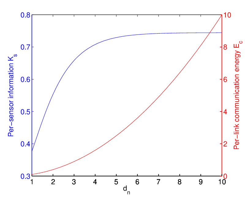
The per-link communication energy can be made arbitrarily small by decreasing the sensor spacing. To investigate the effect of diminishing communication energy $E_{c}$ as $d_{n}\rightarrow 0$, we now consider the asymptotic case in which the node density goes to infinity for a fixed coverage area. In this case, the per-node information decays to zero as $d_{n}\rightarrow 0$ since $\zeta\rightarrow 1/4$ as $d_{n}\rightarrow 0$, and $\mbox{$\mathscr{K}$}_{s}(\zeta)$ and $I_{s}(\zeta)$ converge to zero as $\zeta\rightarrow 1/4$, as shown in Section 3.2. The asymptotic behavior in this case is given by the following theorem.

The finite total information for the infinite density and fixed area model follows our intuition. The maximum information provided by the samples from the continuous-index random field does not exceed the information between $X(x,y)$ and $Y(x,y)$ except for the case of spatially white fields. It is common that the propagation loss factor $\nu>3$ for near field propagation (i.e., $d_{n}\rightarrow 0$). Hence, infinite energy efficiency is achievable as we increases the node density for a fixed area considering only communication energy. Note that the total amount of information converges to a constant as we increases the node density. So, the infinite energy efficiency is achieved by diminishing communication energy as $d_{n}\rightarrow 0$. Considering the sensing energy, however, infinite energy efficiency is not feasible since we have in this case

$$E=n^{2}E_{s}+\Theta(n^{3-\nu})~\mbox{and}~\eta=\frac{c_{5}+o(1)}{n^{2}E_{s}+\Theta(n^{3-\nu})},~~~\nu\geq 2,$$

(30)

as $n\rightarrow\infty$ for fixed coverage area. In this case the sensing energy $n^{2}E_{s}$ is the dominant factor for low energy efficiency, and the energy efficiency decreases to zero with rate $O\left(\mu_{n}^{-1}\right)$. Thus, it is critical for a densely deployed sensor network to minimize the sensing energy or processing energy for each sensor.

In the infinite density model, we have observed that energy is an important factor in efficiency. Now we investigate the change of total information w.r.t. energy. We fix the node density and consider two scenarios to increase the required energy: One is to fix the coverage area also and increase the sensing energy, and the other is to fix the sensing energy and increase the coverage area. We assume that the network size is sufficiently large so that our asymptotic analysis is valid. The energy asymptotic behavior for two scenarios is summarized in the following theorem.

Theorem 6 suggests a guideline for investing the excess energy. It is not efficient to invest energy to improve the quality of sensed samples from a limited area. This only provides the increase in total information in logarithmic scale. Rather the energy should be spent to increase the number of samples by enlarging the coverage area even if it yields less accurate samples.

References

- [1] F. Liese and I. Vajda, “On divergence and informations in statistics and information theory,” IEEE Trans. Inform. Theory, vol. 52, no. 10, pp. 4394-4412, Oct. 2006.
- [2] Y. Sung, L. Tong and H. V. Poor, “Neyman-Pearson detection of Gauss-Markov signals in noise: Closed-form error exponent and properties,” IEEE Trans. Inform. Theory, vol. 52, no. 4, pp. 1354-1365, Apr. 2006.
- [3] Y. Sung, X. Zhang, L. Tong and H. V. Poor, “Sensor configuration and activation for field detection in large sensor arrays,” IEEE Trans. Signal Processing, vol. 56, no. 2, pp. 447-463, Feb. 2008.
- [4] J.-F. Chamberland and V. V. Veeravalli, “How dense should a sensor network be for detection with correlated observations?,” IEEE Trans. Inform. Theory, vol. 52, no. 11, pp. 5099-5106, Nov. 2006.
- [5] A. Anandkumar, L. Tong and A. Swami, “Detection of Gauss-Markov random field on nearest-neighbor graph,” in Proc. 2007 ICASSP, Hawaii, USA, Apr. 2007.
- [6] H. Rue and L. Held, Gaussian Markov Random Fields: Theory and Applicatons, New York: Chapman & Hall/CRC, 2005.
- [7] Y. Sung, H. V. Poor and H. Yu, “Large deviations analysis for the detection of 2D hidden Gauss-Markov random fields using sensor networks,” in Proc. 2008 ICASSP, Las Vegas, NY, Mar. 2008.
- [8] Y. Sung, H. V. Poor and H. Yu, “How much information can one get from a wireless ad hoc sensor network over a correlated random field?,” submitted to IEEE Trans. Inform. Theory, Apr. 2008.
- [9] J. Besag, “On a system of two-dimensional recurrence equations,” Journal of the Royal Statistical Society. Series B, vol. 43, no. 3, pp. 302-309, 1981.
- [10] A. Erdélyi, Higher Transcendental Functions, Vol. II., New York: McGraw-Hill, 1953.
- [11] P. Whittle, “On stationary processes in the plane,” Biometrika, vol. 41, no. 3, pp. 434-449, Dec. 1954.