Static Potentials and the Magnetic Component of QCD Plasma near
Abstract
Static quark-anti-quark potential encodes important information on the chromodynamical interaction between color charges, and recent lattice results show its very nontrivial behavior near the deconfinement temperature . In this paper we study such potential in the framework of the “magnetic scenario” for the near Tc QCD plasma, and particularly focus on the linear part (as quantified by its slope, the tension) in the potential as well as the strong splitting between the free energy and internal energy. By using an analytic “ellipsoidal bag” model, we will quantitatively relate the free energy tension to the magnetic condensate density and relate the internal energy tension to the thermal monopole density. By converting the lattice results for static potential into density for thermal monopoles we find the density to be very large around Tc and indicate at quantum coherence, in good agreement with direct lattice calculation of such density. A few important consequences for heavy ion collisions phenomenology will also be discussed.
pacs
12.38.Mh, 25.75.-q, 47.75.+fI Introduction
The interaction potential between static quark and anti-quark pair is a traditional observable to study the quark confinement mechanism in QCD. It was originally inferred from heavy meson spectrum and Regge trajectories, and has then been extensively studied in lattice gauge theories, for reviews see e.g. [1, 2]. Its vacuum () form is well known, usually represented as a sum of a Coulomb part , dominant at small separation between , and a linear part dominant at large separation (see the black solid curve in Fig.1). The latter implies the confinement of quarks and has been interpreted in terms of chromo-electric flux tube (or “string”) formation between well-separated pair. The so-called string tension in the vacuum () has been consistently determined by different methods to be
| (1) |
With current RHIC and future LHC experimental programs exploring excited hadronic matter and quark-gluon plasma (QGP) at increasing temperature , it is very important to know the finite form of the static potential, which has recently been calculated by means of the lattice QCD, see e.g. [3, 4, 5]. At finite temperature, there are actually two potentials associated with a pair separated by distance : one is the free energy and the other is the internal energy , with the difference related to the entropy generated in the medium by the pair, i.e.
| (2) |
What is directly evaluated on lattice is the free energy from which the corresponding and can be inferred [3]. While at there is no entropy and the free and internal energies are identical, splitting between the two shall be expected at and may carry key information about the medium and deconfinement transition near .
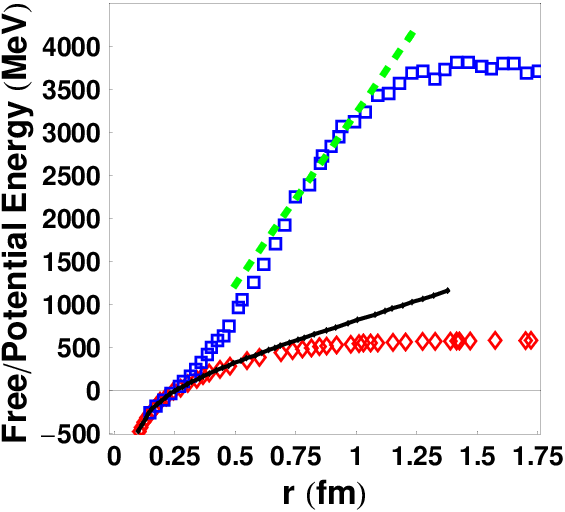
The lattice results indeed show remarkably different potentials and near (see e.g. Fig.1-4 in
[6] and also here Fig.1 adapted from [3]). In particular let us emphasize two important points.
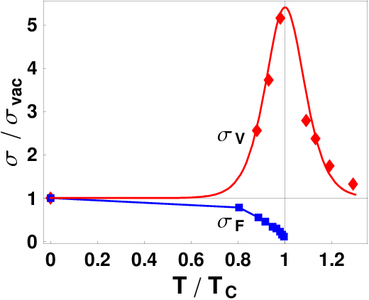
(i) The tensions (slopes of the potentials at about ) have very different temperature dependeces: while the tension of the free energy decreases with , to near zero at (an expected signal of deconfinement), the tension of the internal energy remains nonzero till about , with a peak value at about 5 times (!) the
vacuum tension (see Fig.2).
(ii) This drastically different behavior persists to very large distances, where linear behavior changes to saturated values.
Near the internal energy flattens to huge asymptotic value at large , e.g.
at with the corresponding
entropy
implying huge number of states involved, .
These features indicate strikingly strong interaction between the static color charges and the medium near , which persists into the deconfined phase.
Such static potentials at finite are closely connected with a number of phenomenological issues. For example, the consequence of these features for the survival of quarkonium in deconfined plasma is much debated, e.g. on what/which potential should be used [7, 8, 9]. If, as suggested in [10, 11], the internal energy is used, state would exist even in the deconfined plasma in . Persistence of some baryonic states above is also indicated by other observable like the baryonic susceptibilities[12, 13]. These potentials also imply significant interaction energy in the quark-gluon plasma and in the many body context this may lead to a large classical plasma parameter (defined as the ratio of average interaction energy to average kinetic energy): indeed the value in sQGP has been estimated to be above one (about 3) and thus in a typical liquid regime (see for example [14, 15, 16]). If so, QGP would be a strongly coupled Coulombic liquid, in agreement with the strong collective flow observed at RHIC, see more in reviews [17, 18]. Apart from QGP phenomenology, it is important to understand the microscopic origin of the potentials, especially the strong splitting between two potentials and the large energy/entropy associated with the static pair near . Earlier attempts can be found in e.g. [19, 20, 21].
In this paper we will specifically focus on the “tensions” and (as shown in Fig.2) related to the linear part of the potentials (while leaving the discussion of “screening” behavior at very large distances to further studies). We will provide an explanation in the framework of the magnetic scenario of QCD plasma near [15, 22, 23, 25, 24]. In such a scenario, the near QCD plasma is strongly influenced by the magnetic component, made of relatively light and abundant chromo-magnetic monopoles. Those are quasiparticles above which undergo the Bose-Einstein condensation (BEC) below , enforcing color confinement (for reviews see e.g. [26, 27]). Two key points of the present model for the potentials are: First, we identify the free energy as been probed by an adiabatically “slow separation” process while the internal energy by a “fast separation” process. Second, we further relate the linear part of potentials with the flux tube formation, enabled by condensed monopoles below while thermal monopoles above , between the pair during the separation process [28], and relate the free/internal energy tensions with the condensed/thermal monopoles respectively. These ideas will be elaborated more in Section II and III.
The rest of the paper is structured as follows. In Section-IV we will develop an analytic “elliptic flux bag” model for a static charge-anti-charge pair by solving the Laplace equation for electric field inside it. This allows to get the potentials correctly interpolating between Coulomb at short distance and linear behavior at larger distance. The model will then be used in section-V to determine the free and potential energies and relate the extracted and with the monopole condensate and the thermal monopole density, respectively. Finally we summarize the results in Section-VI.
II Free v.s. Internal Energy and Slow v.s. Fast Separation
Let’s start by examining the difference between the free energy and the internal energy. We already introduced the effective string tensions and as the slopes of linear parts in and respectively, and emphasized their quite different -dependencies shown in Fig.2. While vanishes at , survives to at least . While monotonously decreases with , peaks at to a maximal value of 5 times the vacuum string tension . What is the difference in the meaning of and , and why do they have such different -dependence? As has been emphasized in [10], the free and internal energies actually correspond to slow and fast (relative) motion of the charges, respectively. Let us explain this idea in more details.
Consider the “level crossing” phenomena, occurring while the separation between charges is changed. Suppose a pair of static charges (held by external “hands”) are moved apart in thermal medium at certain speed . For each fixed , there are multiple configurations of the medium populated thermally. When is changed, the energies of these configurations are crossing each other, and at each level crossing there is certain probability to change between the levels, depending on the speed of separation . If the motion is adiabatically slow, then all the level crossing processes happen with probability : in thermodynamical context this leads to maintained equilibrium and maximal entropy/heat generation. If however the pair is separated very fast, then the level crossing is suppressed and the medium is no longer in equilibrium with the pair. The amount of entropy generated is less than in the adiabatic case. In the extreme case one may expect that the pair, if moving on a time scale much much shorter than the medium relaxation time scale, decouples from the media and produce negligible entropy. It is plausible, therefore, to identify the adiabatic limit as probing the free energy measured on the lattice with the presence of static pair. The “internal energy” , on the other hand, is different from by subtracting the entropy term and thus can be probed in the extremely fast limit in which possible transitions among multiple states via level crossing do occur and no entropy is generated.
We emphasize that such phenomenon in thermal medium is a direct analogue of what exists in pure quantum mechanical context. Perhaps the oldest example is the so called Landau-Zener phenomenon [29, 30] of electron dynamics during the vibrational motion of two nuclei in a diatomic molecule. Specific electron quantum states are defined at fixed (the separation between two nuclei) with energies , and certain levels cross each other at specific value of . The issue is the probability of the transition during such crossing of two levels. Consider two levels with their energies given approximately by and near the crossing point. When the two nuclei approach the crossing point adiabatically slowly , the electrons always change from one state to the other selecting the state at any . If the two nuclei have fast relative motion then the transition between the two levels at crossing point is suppressed. More quantitatively, Landau and Zener showed that the probability to remain in the original state (i.e. no transition) is exponentially small at small velocity
| (3) |
where is the off-diagonal matrix element of a two-level model Hamiltonian describing the transition between the two levels.
III Stable and Metastable Flux Tubes
We now turn to the possible microscopic origin of the linear rise in both potentials. Let’s start with the “dual superconductor” model for QCD confinement in the vacuum, introduced by t’Hooft-Mandelstam [31] and well supported by extensive studies in lattice QCD. In this model, certain “magnetically charged” condensate (i.e. a magnetic superconductor) occupies the vacuum and expels the electric flux between into a stable flux tube by forming magnetic super-current on tube surface, known as (dual) Meissner effect. Such flux tube naturally gives rise to a linear potential and the vacuum string tension is thus identified with energy per unit length of such flux tube, mathematically described by the well-known Abrikosov-Nielsen-Olesen (ANO) solution [32] (for reviews and further references see e.g. [33, 1, 2, 34]). What happens at finite T then? With increasing T, the free energy tension decreases and eventually the linear part in free energy disappears at , signaling the deconfinement transition. Since the flux tube and free energy tension is a direct consequence of the magnetic condensate, the decrease of toward is naturally interpreted as the gradual “melting” of the magnetic condensate due to thermal excitations: similar phenomena is known for the usual superconductor in condensed matter systems.
Now, where does the linear part in internal energy (and the associated tension ) come from? In particular, why does it persist even above ? The answer first proposed in [15] relates it to the “normal” monopoles, as opposed to the BEC condensed monopoles existing only below . Such thermal monopoles can also expel the electric flux into (meta-stable) flux tube by forming a magnetic current (which may suffer from dissipation) on the tube surface: its dual phenomenon, i.e. magnetic flux tube formation in thermal electron plasma is well know in classical (e.g. solar) plasma physics. Specific condition for the persistence of the electric flux tube in a magnetic plasma was further developed in [28], for infinitely long flux tubes. There it has been found that “normal” monopoles are much less effective for this task as compared with “super” monopoles, but nevertheless able to mechanically stabilize the flux tube provided high enough density of these thermal monopoles. What has not been previously considered is the mechanism for dynamical formation of flux tube between a pair with finite separation.
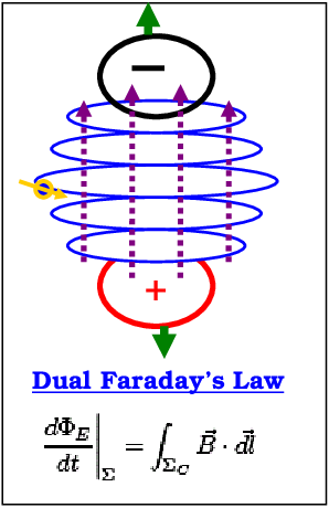
Here we provide a dynamical explanation of why large energy, growing approximately linearly with length, appears in a magnetic plasma when a pair of two electric charges are separated with certain speed , see sketch of the setting in Fig.3. The answer lies in the Maxwell equations (with the presence of magnetic sources, see e.g.[42]), in particularly the Faraday’s law which relates the circulation of the magnetic field over a closed contour with the change of electric flux penetrating the enclosed area. As an electric charge moves through the loop, rotating magnetic field in the magnetic medium leads to solenoidal magnetic current (a “magnetic coil”). In the confined phase this current, after relaxation, becomes the persistent super-current, remaining forever without loss: thus the free energy has a linear term for . In a deconfined plasma phase this is impossible, thus : the solenoidal “magnetic coil” created in the fast process has only normal magnetic current, which is a meta-stable flux tube and eventually disappears due to dissipation. Yet it is still generated: thus is nonzero and there is splitting between free and internal energy.
Let us emphasize again the different roles of the super and normal magnetic components. The former responds quantum mechanically as a whole and does not generate any entropy nor contribute to the splitting. the latter, however, has finite relaxation time and nonzero dissipation, “feels” the different time scales involved in the slow/fast processes, and therefore is responsible for entropy generation and the splitting between free and internal energy. In short, the tells us about the super component only, while the difference tells us about the normal component. One arrives at the following picture for an evolving magnetic medium: with increasing the monopole ensemble starts as a monopole condensate and continuously evaporates into a mixture of both condensed and thermal monopoles; at the condensate melts entirely into a normal component of thermally excited monopoles. If so, the thermal monopoles are expected to be most important in the temperature range where the splitting is most significant.
We end this Section with discussions on a few important phenomenological implications of the “dual Faraday effect” and the meta-stable flux tube. First, it means that magnetic monopoles may induce new mechanism of (electric) jet energy loss particularly near . In the jet quenching process, a very fast electric parton (quark or gluon) penetrates the bulk medium through various phases and thus may create behind it the above discussed “magnetic coil” in the near region where there are abundant thermal monopoles to be accelerated solenoidally by field due to the fast moving electric jet and thus take enormous amount of energy away from the jet. Such near- enhancement of jet quenching has been first suggested by us in [35] and found to be strongly favored by the azimuthal anisotropy data of jet quenching. Second, it also implies specific patterns of multi-particle correlations if such flux tubes can be created and protected by monopoles in heavy ion collisions, as elaborated first in [36]. One example is related to what happens to the flux tube created by a fast jet: clearly the monopoles forming the “coil” will subsequently collide with the bulk thermal matter, with their energy being converted and distributed into the bigger volume: this may possibly be the beginning of “conical flow” process suggested in [37]. The other example concerns the narrow-azimuthal-angle long-range-rapidity correlations known as “ridge” which seems originating from certain local initial fluctuation seeds, but its narrowness in angle may be possibly preserved till the end of long bulk evolution only if certain mechanism like the flux tube by the thermal monopoles protects the initial seed from acoustic expansion (see detailed discussions in [36]). The existence of meta-stable flux tubes in the near plasma (and their associated large entropy) may also bear relevance to the observed cluster correlations [38]. While the existence and dynamical formation of such flux tubes are studied in [28] and here, another very important question (particularly for phenomenology) is its life time, i.e. the flux tube decay and the end products. This problem has recently been partially addressed in [39] where a relatively short life time is found in the classical treatment. On one hand from hydrodynamic modeling we know the near plasma has very small shear viscosity which indicates short mean free path and frequent scattering, while on the other hand for the magnetic currents to last long and hold the flux tube they better do not scatter too often: such a dilemma might be resolved if the thermal monopoles become really coherent over large distance at close to and the lattice study supports such coherence [40]. These questions will be studied further elsewhere.
IV Electric Field Solution in the Ellipsoidal Bag
In this Section we will solve the Maxwell equation for electric field induced by a pair of static charge-anti-charge separated by a distance along axis ( sitting at ), with a special “tangent boundary condition” (T.B.C.) on the boundary surface , i.e.
| (4) | |||
The model itself is a version of an old idea known as the Bag Model used for light hadrons [41] at , now generalized to give an approximate description of the electric field configuration between static in the chromo-magnetic medium at finite temperature.
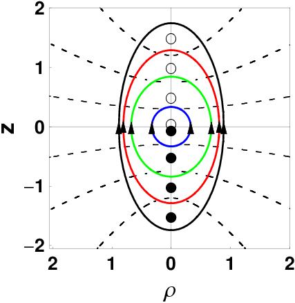
A simplification we use is that the boundary is approximated by a rotational ellipsoid with the two charges at its focal points. This boundary shape can be specified by a single parameter , the ellipticity. Such boundary is very conveniently parameterized in terms of the parabolic coordinates system , which we use: see Appendix A for necessary formulae related to it. In Fig.4 we show a few ellipsoidal shapes with parameters (from inside to outside) to be ,,, respectively, the dashed lines indicate constant- curves (for case) with (from top to bottom) , the solid/empty circles indicate the positions of positive/negative charges, and the arrows indicate the tangent electric fields on the boundary.
We follow the standard method in classical electrostatics, see for example [42]. First, we rewrite (4) in coordinates for solutions with axial symmetry, i.e. assuming independent of angle
| (5) |
The last line in the above is an expansion of the -dependence in terms of Legendre functions which in the interval form a set of orthogonal and complete basis functions. Similarly, we do the expansion for the -dependence of :
| (6) |
Then by simply comparing the coefficients of on both sides of Eq.(5) we obtain the equations for the functions defined in :
| (7) |
while the boundary condition in Eq(4) now becomes
| (8) |
with the parameter specifying the boundary surface . The solutions are given in terms of the Legendre functions of the first and second kinds:
| (9) | |||
The full electrostatic potential is then given by
| (10) |
We’ve used the Neumann expansion of Legendre functions (see e.g. [45]) to write down the second equality: in there the first two terms are nothing but the usual Coulomb potentials by the charges, while the last summation term reflects the nontrivial boundary contribution. At very large the summand terms go asymptotically like , so with satisfying , the summation is guaranteed to converge. The electric field has been calculated using (A4) and the expression is quite lengthy which we skip showing here.
The volume occupied by the electric field (i.e. the ellipsoid bulk within ) is given by
| (11) | |||||
And the total electric field energy in this volume is given by
| (12) |
The is the familiar self-interaction of the two charges which we discard. The “real” interactional energy consists (again) a Coulomb piece and a boundary modification.
We conclude this section by one remark: so far the two key variables and remain free parameters: they will be related in the next section.
V The Free and Internal Energy of the Charge Pair
With the solutions of electric field in the ellipsoidal bag (characterized by two parameters and ) from preceding Section, we now examine the dynamic formation of such bag when separating a pair of from zero to a finite distance . The key point is that for a given , the bag boundary shall be optimized so that the “cost” for creating such a configuration is minimized. Furthermore we study two settings: slow and fast separation of the to a finite distance , with the outcome being respectively the free and internal energy associated with the pair. With slow separation, the free energy increase associated with the pair shall be minimized, and the dominant contributions to the free energy include both the electric field energy stored inside the bag and the energy needed to exclude the monopole condensate out of the bag volume (noting that for both there is no entropy associated and for thermal monopoles their contribution to free energy in the slow separation process largely cancels out between energy and entropy). With fast separation, the energy increase shall be minimized, and the dominant contributions to the energy include both the electric field energy stored inside the bag and the energy deposited to the thermal monopoles via the dual Faraday effect. We will calculate both processes in the rest of this Section and make connections with the lattice data.
V.1 Free Energy from Slow Separation
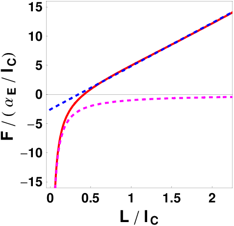
As afore-discussed, when the pair is separated in an adiabatically slow way, the super component of the magnetic medium i.e. the monopole condensate will be expelled entirely (in an idealized picture) out of the volume occupied by electric field. Suppose the condensate has a negative energy density (thus a positive “bag pressure”), then the overall change in free energy brought about by separating the pair will be
| (13) |
Now for given separation distance and bulk temperature , we determine the physical boundary of flux bag by minimizing the above , i.e. the physical boundary satisfies:
| (14) |
Combining the above with Eq.(11,12) we then obtain
| (15) |
where we have introduced a length scale
| (16) |
with . This
equation could be solved easily by numerics. For each with the
above determined , we obtain via (13)
the free energy associated with the pair as a function of
separation , shown in Fig.5(a). It turns
out to be Coulomb at short distance(see the magenta dashed curve)
plus linear at large distance(see the blue dashed line). The
occurrence of a linear part is due to the physical effect that for
large the medium pressure (with which the electric field has
to balance) limits the transverse size of flux bag (where the
field gets weak as increases) to saturate rather than grow
forever: thus the bag shape approaches a cylinder. Mathematically,
as one finds but . In Fig.4
the four bag shapes are at growing with determined as
in the above, which clearly
shows the shape becomes more and more cylindrical at large .
By fitting the dimensionless slop of the linear part in Fig.5(a) we obtain the free energy string tension :
| (17) |
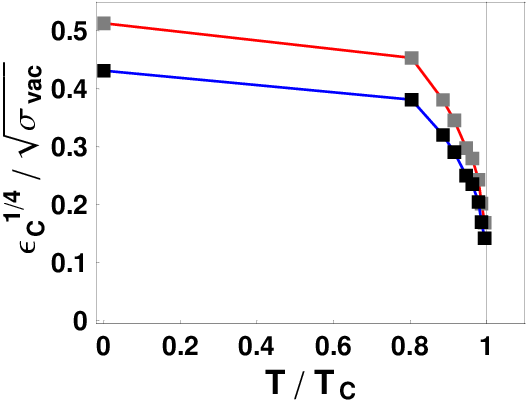
Inversely, since we know from lattice as shown in Fig.2, from the above formula we can infer the -dependence of the monopole condensate energy density : see Fig.5(b). The two curves are for being 0.5(upper) and 1(lower) respectively. In both cases, decreases with and drops abruptly close to . The interpretation is natural: toward the monopole condensate becomes less and less due to increasing thermal excitations and eventually dies out around .
A connection can be made between our result (17) and the dual superconductor model (also known as Abelian Higgs model) of vacuum confinement [33]. In that model, a quadratic Higgs potential leads to a Higgs condensate (the prototype of postulated monopole condensate) (with dimension of mass). By solving ANO flux tube a string tension is obtained in the form with the coefficient determined by gauge and Higgs coupling constants and . On the other hand the Higgs potential implies that the condensate has a negative energy density , thus one arrives at a similar relation between string tension and condensate energy density: in that model with the coefficient to be determined numerically for given coupling parameters, see e.g. [43]. While that model works primarily at , our model for extends to finite T.
V.2 Internal Energy from Fast Separation
Now we study the case of separating the two charges to a finite distance within a time much smaller than the relaxation time of the surrounding thermal bath. In particular we focus on the region about , in which the normal component of thermal monopoles becomes substantial and dominant while the super component becomes less and less.
During such fast process, each monopole originally in the volume to be occupied by the electric filed (i.e. the ellipsoidal bag) will get a ”kick” due to the dual Faraday effect (see Fig.3) but have no time to release this energy into the surrounding medium. Suppose the positive charge is moved along -axis from to in (and correspondingly the negative one from to ), then the electric flux penetrating the plane changes from 0 to , thus generating a magnetic dynamical voltage . For a monopole at a transverse distance from axis, the force is , thus it gets the ”kick” and obtains a momentum , forming strong non-thermal and non-super magnetic currents. For a bag formed after separation, the total kinetic energy passed to the monopoles in the flux bag is obtained by integration over the bag volume (with ):
| (18) | |||||
We emphasize in the above only the monopole density enters as a property of the medium depending on , while other equilibrium properties of the medium shall not be ”felt” in such fast process.
Now the total energy change during such process includes the electric field energy in the bag volume, the energy for expelling the monopole condensate (if there is any) out of the volume, and the kinetic energy delivered to the normal monopoles, which are summed to be . The last new term due to the thermal monopoles will then partly convert into entropy after they interact with the medium particles at large for a time longer than the relaxation, ultimately causing the splitting between free/internal energy. Since the condensate term becomes very small close to (as we showed in previous subsection) and vanishes above , we neglect it here for simplicity, i.e. . To obtain the physical value , we need to minimize according to , which leads to
| (19) |
This can be written as
| (20) |
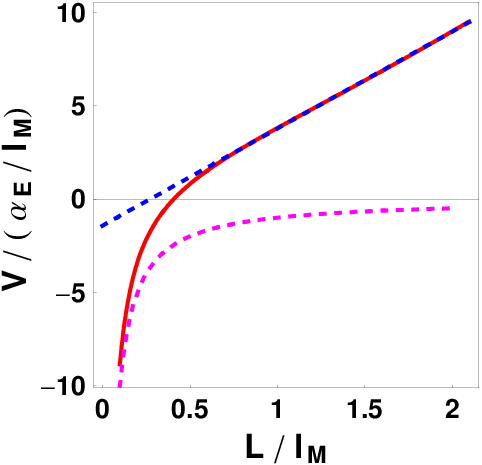
Here we introduced a different length scale . Not surprisingly we find the internal energy, shown in Fig.6(a), to be a Coulomb at short distance(see the magenta dashed curve) plus linear at large distance(see the blue dashed line).
Now the string tension in the internal energy is given by the following formula:
| (21) |
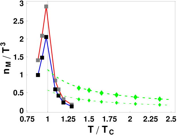
Since we know from lattice data in the region, by the above formula we can convert into thermal monopole density in the same region: see the two curves(connecting box symbols) for being 0.5(upper, red) and 1(lower, blue) respectively in Fig.6(b). We also show an independent information on the thermal monopole density above from lattice study in [25] in Fig.6(b) as green curves(connecting diamond symbols): the lower one is the original data for in [25], while the upper one is an extrapolation to by the simple scaling for monopole species (i.e. twice more monopoles in than in ), with both curves extended toward according to the fitting formula (and twice in the upper one for ) in [25]. The comparison shows reasonably good agreement between our estimates for the thermal monopole density from string tension and the measured density by directly identifying the thermal monopoles on the lattice.
A few comments are in order: (i) for the density quickly grows toward while at the same time results from previous subsection show rapid dropping of condensate density in the same region, which strongly indicates the scenario that close to monopole condensate is continuously and substantially getting excited into thermal monopoles; (ii) around we see our results connect well to the higher lattice data with reasonable values of coupling ; (iii) cooling down to we find the monopole density quickly rising almost by an order of magnitude; (iv) the strongly increasing density also suggests rapid increase of magnetic screening toward , which is in agreement with lattice results [44].
A particularly interesting feature is that the (normalized) density increases roughly by one order of magnitude from down to , with the number much larger than even a Stefan-Boltzman gas. This indicates that near the monopoles should be very light, and furthermore their interactions should make it beneficial in energy to have a large number of monopole-anti-monopole pairs. The monopoles are so dense and light that they become the dominant component in the near- plasma and presumably become quantum coherent, and eventually reach the condensation point at (see most recent lattice results in [40] showing evidences for such a scenario). It has been suggested that these thermal monopoles near seem to form a densely packed liquid [22][25].
VI Summary
In this paper, we have argued that the free energy and internal energy can be probed by slow and fast separation of the pair, respectively. Furthermore we have identified the linear part in both potentials with flux tube formation between the pair: for free energy as probed by slow separation, there is stable flux tube protected by magnetic super-current due to condensed monopoles which has no dissipation and exists below ; for internal energy as probed by fast separation, there is meta-stable flux tube protected by magnetic normal current due to thermal monopoles which are very dense in the region and generate large entropy (the splitting between free and internal energy) via dissipation on longer time scale. Based on these ideas we have solved analytically the elliptic bags and provided expressions for the potentials at all separations, which happen to describe the data very well.
The main outcome from our study of the static potentials is the particular relations we suggest between the free energy and internal energy measured on the lattice and the densities of the condensed and “normal” monopoles: see Eqs.(17) and (21). Since those densities can be directly obtained from the lattice configurations, one may check if these relations are correct or not. Such further tests of the “magnetic scenario”[15, 23] for the near QCD plasma are rather straightforward and should be performed.
Acknowledgements
The work of JL was partially supported by the Director, Office of Energy Research, Office of High Energy and Nuclear Physics, Divisions of Nuclear Physics, of the U.S. Department of Energy under Contract No. DE-AC02-05CH11231. The work of ES was supported in parts by the US-DOE grant DE-FG-88ER40388.
Appendix A
In this Appendix we briefly list the parabolic coordinates formulae needed for the calculation in Sec.2.
The coordinates we use are with two focal points at , which are related to cylindrical coordinates by
| (A1) |
The variables are defined in the following domains: , , . Writing , we have
| (A2) |
The Laplacian is given by
| (A3) | |||||
Finally the gradient is given by
| (A4) |
For more details one could consult books such as [45].
References
- [1] G. S. Bali, Phys. Rept. 343, 1 (2001) [arXiv:hep-ph/0001312].
- [2] J. Greensite, Prog. Part. Nucl. Phys. 51, 1 (2003) [arXiv:hep-lat/0301023]; R. Alkofer and J. Greensite, J. Phys. G 34, S3 (2007) [arXiv:hep-ph/0610365].
- [3] O. Kaczmarek and F. Zantow, Phys. Rev. D 71, 114510 (2005) [arXiv:hep-lat/0503017]; arXiv:hep-lat/0506019.
- [4] O. Kaczmarek, F. Karsch, E. Laermann and M. Lutgemeier, Phys. Rev. D 62, 034021 (2000) [arXiv:hep-lat/9908010]; O. Kaczmarek, F. Karsch, P. Petreczky and F. Zantow, Phys. Lett. B 543, 41 (2002) [arXiv:hep-lat/0207002]; O. Kaczmarek, F. Karsch, P. Petreczky and F. Zantow, Nucl. Phys. Proc. Suppl. 129, 560 (2004) [arXiv:hep-lat/0309121].
- [5] P. Petreczky and K. Petrov, Phys. Rev. D 70, 054503 (2004) [arXiv:hep-lat/0405009].
- [6] O. Kaczmarek and F. Zantow, PoS LAT2005, 192 (2006) [arXiv:hep-lat/0510094].
- [7] C. Young and E. Shuryak, Phys. Rev. C 79, 034907 (2009) [arXiv:0803.2866 [nucl-th]]. C. Young and E. Shuryak, arXiv:0911.3080 [nucl-th].
- [8] X. Zhao and R. Rapp, Phys. Lett. B 664, 253 (2008) [arXiv:0712.2407 [hep-ph]].
- [9] A. Mocsy and P. Petreczky, Phys. Rev. D 77, 014501 (2008) [arXiv:0705.2559 [hep-ph]].
- [10] E. V. Shuryak and I. Zahed, Phys. Rev. C 70, 021901 (2004) [arXiv:hep-ph/0307267]; Phys. Rev. D 70, 054507 (2004) [arXiv:hep-ph/0403127].
- [11] J. Liao and E. V. Shuryak, Nucl. Phys. A 775, 224 (2006) [arXiv:hep-ph/0508035].
- [12] C. R. Allton et al., Phys. Rev. D 71, 054508 (2005) [arXiv:hep-lat/0501030]; R. V. Gavai and S. Gupta, Phys. Rev. D 72, 054006 (2005) [arXiv:hep-lat/0507023].
- [13] J. Liao and E. V. Shuryak, Phys. Rev. D 73, 014509 (2006) [arXiv:hep-ph/0510110].
- [14] B. A. Gelman, E. V. Shuryak and I. Zahed, Phys. Rev. C 74, 044908 (2006)[nucl-th/0601029]; Phys. Rev. C 74, 044909 (2006)[nucl-th/0605046].
- [15] J. Liao and E. Shuryak, Phys. Rev. C 75, 054907 (2007) [arXiv:hep-ph/0611131].
- [16] C. Ratti and E. Shuryak, arXiv:0811.4174 [hep-ph].
- [17] M. Gyulassy and L. McLerran, Nucl. Phys. A 750, 30 (2005); E. V. Shuryak, Prog. Part. Nucl. Phys.53, 273 (2004) [hep-ph/0312227]; Nucl. Phys. A 750, 64 (2005).
- [18] E.V.Shuryak, arXiv:hep-ph/0608177; arXiv:hep-ph/0703208.
- [19] D. Antonov, S. Domdey and H. J. Pirner, Nucl. Phys. A 789, 357 (2007) [arXiv:hep-ph/0612256].
- [20] E. Megias, E. Ruiz Arriola and L. L. Salcedo, Phys. Rev. D 75, 105019 (2007) [arXiv:hep-ph/0702055].
- [21] A. Beraudo, J. P. Blaizot and C. Ratti, arXiv:0712.4394 [nucl-th].
- [22] J. Liao and E. Shuryak, Phys. Rev. Lett. 101, 162302 (2008) [arXiv:0804.0255 [hep-ph]].
- [23] M. N. Chernodub and V. I. Zakharov, Phys. Rev. Lett. 98, 082002 (2007) [arXiv:hep-ph/0611228]; arXiv:hep-ph/0702245.
- [24] M. N. Chernodub, K. Ishiguro, A. Nakamura, T. Sekido, T. Suzuki and V. I. Zakharov, PoS LAT2007, 174 (2007) [arXiv:0710.2547 [hep-lat]].
- [25] A. D’Alessandro and M. D’Elia, arXiv:0711.1266 [hep-lat].
- [26] E. Shuryak, arXiv:0804.1373 [hep-ph]. E. Shuryak, Prog. Part. Nucl. Phys. 62, 48 (2009) [arXiv:0807.3033 [hep-ph]]. E. Shuryak, Nucl. Phys. Proc. Suppl. 195, 111 (2009).
- [27] J. Liao and E. Shuryak, J. Phys. G 35, 104058 (2008) [arXiv:0804.3102 [hep-ph]]. J. Liao and E. Shuryak, arXiv:0809.2419 [hep-ph].
- [28] J. Liao and E. Shuryak, Phys. Rev. C 77, 064905 (2008) [arXiv:0706.4465 [hep-ph]].
- [29] L. D. Landau and E. M. Lifshitz, “Quantum Mechanics”, 3rd ed., Butterworth-Heinemann, 1981.
- [30] L. D. Landau, Physics of the Soviet Union 2: 46¨C51 (1932). C. Zener, Proceedings of the Royal Society of London, Series A 137 (6): 696¨C702 (1932). For a concise introduction see e.g.: C. Wittig, J. Phys. Chem. B 109, 8428 (2005).
- [31] S. Mandelstam, Phys. Rept. 23, 245 (1976); G. ’t Hooft, “Topology Of The Gauge Condition And New Confinement Phases In Nonabelian Nucl. Phys. B 190, 455 (1981).
- [32] A.A. Abrikosov, Sov. Phys. JETP 32, 1442 (1957); H.B. Nielsen and P. Olesen, Nucl. Phys. B 61, 45 (1973).
- [33] G. Ripka, “Dual superconductor models of color confinement”, Lecture notes in physics, Vol. 639, Springer Berlin / Heidelberg 2004; arXiv:hep-ph/0310102.
- [34] A. Di Giacomo, Prog. Theor. Phys. Suppl. 131, 161 (1998) [arXiv:hep-lat/9802008]; A. Di Giacomo, arXiv:hep-lat/0310023.
- [35] J. Liao and E. Shuryak, Phys. Rev. Lett. 102, 202302 (2009) [arXiv:0810.4116 [nucl-th]].
- [36] E. Shuryak, Phys. Rev. C 80, 054908 (2009) [Erratum-ibid. C 80, 069902 (2009)] [arXiv:0903.3734 [nucl-th]].
- [37] J. Casalderrey-Solana, E. V. Shuryak and D. Teaney, J. Phys. Conf. Ser. 27, 22 (2005) [Nucl. Phys. A 774, 577 (2006)] [arXiv:hep-ph/0411315].
- [38] B. Alver et al. [PHOBOS Collaboration], Phys. Rev. C 75, 054913 (2007) [arXiv:0704.0966 [nucl-ex]]. B. Alver et al. [PHOBOS Collaboration], Phys. Rev. C 81, 024904 (2010) [arXiv:0812.1172 [nucl-ex]].
- [39] C. Faroughy and E. Shuryak, arXiv:1004.2890 [hep-ph].
- [40] A. D’Alessandro, M. D’Elia and E. V. Shuryak, Phys. Rev. D 81, 094501 (2010) [arXiv:1002.4161 [hep-lat]].
- [41] A. Chodos, R. L. Jaffe, K. Johnson, C. B. Thorn and V. F. Weisskopf, Phys. Rev. D 9, 3471 (1974).
- [42] J. D. Jackson, Classical Electrodynamics (3rd edition), John Wiley & Sons, Inc. (1999).
- [43] M. Baker, N. Brambilla, H. G. Dosch and A. Vairo, Phys. Rev. D 58, 034010 (1998) [arXiv:hep-ph/9802273].
- [44] A. Nakamura, T. Saito and S. Sakai, Phys. Rev. D 69, 014506 (2004) [arXiv:hep-lat/0311024].
- [45] Z. X. Wang and D. R. Guo, Special Functions, World Scientific, Singapore (1989).