Interfacing light and single atoms with a lens
Abstract
We characterize the interaction between a single atom or similar microscopic system and a light field via the scattering ratio. For that, we first derive the electrical field in a strongly focused Gaussian light beam, and then consider the atomic response. Following the simple scattering model, the fraction of scattered optical power for a weak coherent probe field leads to unphysical scattering ratios above 1 in the strong focusing regime. A refined model considering interference between exciting and scattered field into finite-sized detectors or optical fibers is presented, and compared to experimental extinction measurements for various focusing strengths.
pacs
42.50Ct, 42.50Ex, 42.25Bs1 Introduction
Atom-light interaction at the single quantum level plays an important role in many quantum communication and computation protocols. While spontaneous emission can provide a natural transfer of atomic states into photonic qubits, strong interaction of light with an atom is needed to transfer a photonic qubit into internal atomic degrees of freedom as a stationary qubit. This process is essential to implement quantum light-matter interfaces [1, 2, 3], unless post-selection techniques are used [4].
The common approach to achieve this strong interaction pursued for a long time is to use a high finesse cavity around the atom, in which the electrical field strength of a single photon is enhanced by multiple reflections between two highly reflective mirrors, resulting in a high probability of absorption. Another approach to increase the interaction between an atom and a single photon is simply to focus the light field of a single photon down to a diffraction limited area, motivated by the fact that the absorption cross section of an atom is on the order of the square of the optical wavelength. Recent theoretical research on this matter predicts that the absorption probability may reach the maximal value of 100% for dedicated focusing geometries [5]. In this paper, we study the interaction strength between a two-level system and a tightly focused weak coherent light Gaussian beam, which is simpler to prepare.
Such a system has been theoretically investigated by van Enk and Kimble [6] and they concluded that one can expect only a weak interaction. An experiment on single atom absorption has been carried out a long time ago in the weak focusing regime [7], but recent experimental results with single molecules [8] and atoms [9] showed an interaction strength which exceeded these theoretical predictions by far. In this paper we extend the original theoretical model such that it is applicable in the strong focusing regime and provide experimental data on the extinction by a single atom for various focusing parameters. Extrapolating from there, we find that the interaction strength in between light and an atom can indeed be very strong for realistic focusing geometries.
The paper is organized as follows: In Section 2, we explain how we quantify the interaction strength between an atom and a weak coherent light field, and set out the basic problem. In Section 3, we calculate the field strength at the focus of an ideal lens by considering a Gaussian incident beam for the strong focusing regime. Using this ‘ideal’ focusing field developed in this section, we then obtain an expression for the scattering ratio in Section 4, and for the extinction of a focused light beam by a two-level system in various geometries in Section 5. The theoretical prediction is compared with our experimental results in Section 6.
2 Basic problem
The system that we investigate is a single two-level atom localized in free space illuminated by a focused weak monochromatic light field (probe) with an incident power . The interaction strength of the probe with the atom is directly related to the fraction of power scattered by the atom. Therefore, it seems reasonable to quantify the interaction strength with the ratio of the scattered light power to the total incident power , i.e.
| (1) |

To prepare an atom into a clean two-level system, it is convenient to use optical pumping with circularly polarized light - the optical transition therefore will also be driven by circularly polarized light. The light field itself should have a well-defined spatial profile before it is focused onto the atom with a lens. A circularly polarized, collimated Gaussian beam propagating along the axis (see figure 1) will therefore be the starting point for our work. Its electrical field strength before the lens is given by
| (2) |
where is the radial distance from the lens axis, the waist of the beam, are the unit vectors in transverse directions, and is the field amplitude. The beam carries a total power of
| (3) |
where is the electric permittivity of vacuum, and the speed of light in vacuum. Due to the rotational symmetry the field on the lens axis is always circularly polarized. For an atom that is stationary at the focal point of the lens, the electric field can thus be written as
| (4) |
where denotes the amplitude of the field at the focus. In the long wavelength limit the atom only interacts with the field at the location of the atom. For a field that is resonant with the atomic transition and with an intensity much below saturation, the power scattered by a two-level atom is [10] (see A for more details)
| (5) |
leading to a scattering ratio of
| (6) |
which is exact under weak and on-resonant excitation. To evaluate the the scattering ratio and therefore the interaction strength, one needs to know .
For a weakly focused field where the paraxial approximation holds one finds that
| (7) |
where is the Gaussian beam waist at the focus. This leads to
| (8) |
with the focusing strength
| (9) |
used to fix the focal waist, . With a Gaussian focal spot area , the scattering ratio can also be expressed as , where is the absorption cross section of a two-level system exposed to a resonant plane wave. However, for strongly focused light, the paraxial approximation breaks down, and we need other methods to find .
3 Electrical field in a tight focus
The paraxial approximation breaks down for strongly focused beams both in the expression of the electric field just behind the lens, and in the propagation of this field to the focus. An approach to overcome the propagation problem was reported by van Enk and Kimble in [6]. Their lens model, however, applies only to the weak focusing regime. In the following, we present a lens model to overcome this limitation and propagate the optical field behind the ideal lens into the focal regime and investigate the focal field using their technique numerically. We obtain a closed expression for the electrical field in the focus using the Green theorem for the propagation.
To simplify the expressions in this section, we express the electrical field in dimensionless units, so the electrical field strength of the collimated Gaussian beam entering the focusing lens is given by
| (10) |
where is one of the circular polarization vectors .
3.1 Model of an ideal lens
An ideal converging lens converts a beam with a plane wave front into one with a spherical wave front which converges towards the focal point . Therefore, it can be modeled as a phase plate modifying an incoming field with a radially dependent phase factor into
| (11) |
In paraxial optics, a convenient analytical treatment of Gaussian beams can be obtained assuming a parabolic phase factor,
| (12) |
this was adopted in [6]. However, the conversion of a plane into a spherical wave front corresponds to a phase factor of
| (13) |
which is only approximated by equation (12). On top of this, multiplication of a incoming field with such a phase factor leads to an electrical field which is not compatible with Maxwell equations, since the polarization vector for is not tangential to the wave front anymore.
In view of this, we have to change the local polarization with three requirements in mind [11]: (i) A rotationally symmetric lens does not alter the local azimuthal field component, but tilts the local radial polarization component of the incoming field towards the axis; (ii) The polarization at point P (see Figure 1) after transformation by the lens is orthogonal to the line FP; (iii) The power flowing into and out of an arbitrarily small area on the thin ideal lens is the same. These requirements determine completely the focusing field right after the lens. With the input field in equation (10), one finds (see B for details)
| (14) | |||||
with . In particular, the factor is needed in order to meet requirement (iii).
3.2 Numerical propagation of the field to the focus
The optical field with a converging wave front directly behind the lens needs to be propagated into the focal region to arrive at a field strength of the light interacting with the microscopic system. Various methods can be applied for this purpose. The one implemented in [6] projects the focusing field on an orthogonal set of modes , with cylindrical symmetry (see C for details). This decomposition reads
| (15) |
where the expansion coefficients are given by
| (16) | |||||
with . The Kronecker symbol reflects conservation of angular momentum under the lens transformation [12, 13]. The projection integral has no analytic solution, so the coefficients have to be evaluated numerically.
The (dimensionless) field components in the three polarization components at any point behind the lens are superpositions of contributions from different modes,
| (17) | |||||
| (18) | |||||
| (19) |
We now evaluate the field components for different regions with this method: first directly behind the lens, then on the optical axes to near the focus, and finally in the focusing plane near the focus.
3.2.1 Focusing field reconstruction
As a consistency check, we first evaluate the field components right after the lens (i.e., for ) for a reasonably strong focusing field with corresponding to mm for mm. The relative difference between the reconstructed and original field is less than , a bound limited by our numerical accuracy. A linear combination of the field modes in the form of equations (17) to (19) is compatible with the Maxwell equations, so since there is no significant difference between the original and reconstructed field, the choice in equation (14) for the focusing field is compatible with Maxwell equations even for strong focusing parameters.
3.2.2 Field along the optical axis
The solid line in figure 2 shows the dimensionless intensity for mm, nm and mm (), with a clearly peaked distribution centered at the focus and a depth of field, defined as the full width at half maximum (FWHM), of about 9.5 m. This result is still very close to the much simpler paraxial approximation of a Gaussian beam, with a depth of field of m.
For comparison, we show the result for a focusing field using a parabolic phase factor only, following [6]. The spherical aberration there displaces and spreads the focus, and significantly reduces the maximal intensity in the focal point . This problem becomes even more serious for a larger input waist .

3.2.3 Field in the focal plane
We now examine the field near the focus in more details. Figure 3 shows the field on the focal plane for different focusing strengths. For this, we choose different input waists , but keep =4.5 mm and =780 nm fixed. For comparison, we also show the result for a focusing field according to the paraxial approximation,
| (20) |
with a paraxial focal waist .

For weak focusing (mm) in figure 3a, overlaps completely with the paraxial prediction with negligible and . For an initial waist mm corresponding to and (about 5), discrepancies between the paraxial approximation and the extended model start to appear (Figure 3b). With increasing , the - and polarized field components become stronger for , but an atom localized on the optical axis still only experiences a -polarized field. Figure 3d shows the focused field that maximizes for the parameters in our model. It is obtained with an incident waist mm (). An increase of the incident waist beyond that does not reduce the focal spot size any further due to the diffraction limit. Instead, more energy is transferred to the other polarization components, thus decreasing the magnitude of the .
3.3 Analytical expression for the field in the focal point
An alternative method for propagating the focusing field directly behind the lens is offered by the Green theorem. For given electrical and magnetic fields and on an arbitrary closed surface that encloses a point , the electrical field at this point is determined by [14]
| (21) | |||||
where is the unit vector normal to a differential surface element and points into the volume enclosed by , and is the Green function given by
| (22) |
If point is the focus of an aplanatic focusing field, then the local field propagation wave vector at any point always points towards (away from) point for the incoming (outgoing) field in the far field limit, i.e. when . In this limit, one has
| (23) | |||
| (24) |
In the far field limit, Equation (21) reduces to
| (25) | |||||
Here the surface is divided into two parts, where is the one before the focal plane, and is the surface after the focal plane. The second term in Equation (25) vanishes if we choose to be an infinitely large hemisphere centered at the focus, since in this case is perpendicular to at all points on for an aplanatic field. If we choose as an infinitely large plane that coincides with the ideal lens and adopt the dimensionless incident field in Equation (14), we get
| (26) |
which has an analytical solution
| (27) |
with the incomplete gamma function , and as in Equation (9). The results obtained with the mode decomposition method agree with this expression within computational errors of about 0.1%. The reflects a Gouy phase of [15].
We now restore the field dimensions by multiplication with the amplitude in the center of the collimated Gaussian beam, which can be expressed by the optical power according to equation (3),
| (28) |
resulting in an electrical field amplitude in the focus of
| (29) |
with purely circular polarization. The focal field thus only depends on the input power, the optical wavelength and the focusing strength .
4 Study of the scattering ratio

The electrical field amplitude at the focus for a given excitation power now allows to determine the fraction of the optical power scattered away by a two-level atom or similar microscopic object according to equation (5). With Equation (29), we arrive at
| (30) |
In Figure 4 we show this quantity as a function of the focusing strength . A striking feature of this plot is that, for large enough, exceeds the value of 1, as if more light would be scattered than was incident. However, cannot be interpreted as a scattering ratio anymore if the solid angle subtended by the excitation field is not negligible: in the strong focusing regime, interference between the exciting field and the scattered field must be taken into account. In fact, the physical bound (Bassett limit) is [17]. For our focusing model of the Gaussian beam, we predict a maximal value of for a focusing strength .
For reference, we also show for focal fields derived under the paraxial approximation and for a parabolic wave front model. All models agree in the weak focusing regime, and can reach values on the order of 1, which indicates that by strong focusing, one can accomplish a strong interaction between a light field and a single atom.
5 Extinction as a measurement of scattering
The parameter we have just discussed can be used as a figure-of-merit for scattering experiments. In this section, we go beyond this one-parameter description to provide a detailed model for the experiment we performed [9]. In this experiment, we measured the extinction of the transmitted light beam due to scattering.

Figure 5 illustrates a simple transmission setup with an atom located at the focus of two confocal lenses, where the second lens collects all the excitation power if no atom is present at the focus. The actual measured transmission depends on the area covered by the power detector after the second lens, and can be obtained by considering the interference between the incident probe field and the field coherently scattered by the atom. For a given focusing and collection geometry, the extinction
| (31) |
is maximal for a weak incident probe field in resonance with the transition in the two-level system. The total field at any place is a superposition of the focusing field exciting the atom, and the scattered field:
| (32) |
The spatial dependency of the scattered field is that of a rotating electrical dipole, with an amplitude proportional to the exciting electrical field amplitude , and the total power contained in this dipole radiation must match Equation (5). Far away from the dipole (), this scattered field takes the form
| (33) |
where is the radial unit vector pointing away from the scatterer [10]. The phase reflects the fact that the dipole moment of the atom lags the field by at resonance. The focusing field close to the lenses at takes the form
| (34) | |||||
where is the polar angle between the direction and a point as in figure 1. The phase is adjusted such that the electric field amplitude at the focus is real.
The excitation field and the forward scattered field interfere destructively, as was shown first for the case of an incident plane wave [16, 18, 19], and more recently for arbitrary incident fields [20] with the help of vectorial multipole expansions [21, 22, 23].
5.1 Energy flux through transverse planes
The optical power arriving at a detector behind the atom or a collection lens can be evaluated from the superposition of fields via the time averaged energy flux through a plane with a fixed ,
| (35) |
where is a differential area element of the surface and denotes the real part of .
Far away from the focus, the electromagnetic field can be locally approximated by a plane wave such that , where is a dimensionless unit vector parallel to the local field propagation direction. Both and have spherical wave fronts, i.e., the local propagation directions are parallel. Before the focus we have , while after the focus we have . With these field properties, and with the local transversality, and , the power through the two planes can be expressed with electrical fields only,
| (36) |
The two first terms represent (i) the power of the excitation field, (ii) the power of the scattered field, while the third and fourth term represent (iii) the interference term.
The contribution (i) to is simply the input power,
| (37) |
and the contribution (ii) in these planes,
| (38) |
where is the scattered power as defined previously in Equation (5).
The interference contribution (iii) vanishes for because is purely imaginary, whereas for we get
| (39) | |||||
| (40) |
The negative sign, which comes from both the Gouy phase in the incident field (Equation (34)) and the phase difference between the dipole and local field (Equation (33)), reveals that the scattered light and the incident light interfere destructively after the focus [20]. This integral can be solved in the same way as Equation (26), leading to
| (41) |
Thus, the power flowing through both planes is the same,
| (42) |
This indicates what we mentioned above: a value does not violate energy conservation, the physical bound being rather .
For later on, we should define a measurable extinction as the difference of the transmitted power with and without the atom, divided by the power transmitted without the atom at a location behind the atom, e.g. at :
| (43) | |||||
If the collection lens at is infinitely large, it takes a value of
| (44) |
5.2 Extinction observed with a detector/lenses with finite diameter
Realistic lenses will have a finite size, thus only partly transmit the excitation and scattered light. We now estimate how this obstruction affects the relation between an observed extinction and the inferred scattering ratio .
The first effect of a finite lens aperture radius of the first lens is a reduction of the field at the focus. The Green theorem method for evaluating the focal field via equation (26) still has a closed solution for a finite radius,
| (45) |
with as in Equation (9), and similarly as half the f-number of the lens which is related to the numerical aperture NA of the lens via . This obstruction reduces the scattered power . For realistic lens sizes, however, this is a very small effect. For instance, for we find .
Without the atom, the transmitted power after the collection lens is given by
| (46) |
The transmitted power in absence of an atom is thus very close to for . The contribution (iii) of the interference terms to the forward power is now given by
| (47) |
and the contribution (ii) of the scattered light by
| (48) | |||||
| (49) |
The extinction measurable with a finite aperture lens thus is
| (50) |
If the lenses fully accommodate the Gaussian incident beam, say , then this can very well be approximated by
| (51) |
where .
We can also quantitatively evaluate the reflectivity of a single atom in this strong focusing regime, which was recently found to be possibly very large [20]. The scattered power recollected by the input lens is also given by Equation (48), thus the ’single atom reflectivity’ with a Gaussian beam profile is
| (52) |
We conclude that the measured extinction presents a lower bound to the scattering ratio if the collection lens fully collects the probe after the focus. For a small numerical aperture of the collection lens, as expected, whereas for a large collection aperture (corresponding to a small loss factor ), a reduced extinction should be observed.
5.3 Extinction observed with a detector behind a single mode fiber
The symmetrical arrangement of the focusing and collection lens, and the typical preparation of a Gaussian excitation beam by an optical fiber suggests that the light could also be collected by a single mode optical fiber. The confinement of the light field into waveguides with well-defined mode functions makes the atom-focusing arrangement an independent building block for ’processing’ electromagnetic fields.
The amplitude of the light field collected into the optical fiber is again given by the sum of the excitation and scattered field, picked up by the optical fiber. This amplitude can be obtained by projecting the field onto the field mode of the optical fiber. This projection can be carried out with the scalar product
| (53) |
where the integration plane is chosen such that both and are far away from a focus, is the local propagation direction of the mode function , and the normal vector on the plane . This integration can be carried out at any convenient location as long as it captures the mode function. The scalar product in Equation (53) is written such that it resembles the form of the power integral in planes in Equation (36), so we can conveniently use the integrations carried out earlier. Thus, the integration plane is chosen at , directly before the collection lens.
In the experiment, the excitation mode is matched to the collecting single mode fiber. Correspondingly, we define the target mode function to be the same as that of the excitation mode of in equation (34). With the normalization condition we simply can set
| (54) |
With this normalization, the square of the projection coefficient has the dimension of a power. Thus, the optical power of the field coupled into the fiber with a scattering atom present is given by
| (55) | |||||
The first scalar product is determined by the mode normalization. The second one, , represents the projection of the scattered field onto the collection mode. Modulo the normalization constant , it is identical to half the interference contribution in Equation (39), whose explicit expression was given in Equation (41). Therefore we find
| (56) |
In the weak focusing regime where , this translates again into an extinction For a focusing parameter , we get a maximal extinction of . For the light scattered back into the excitation mode, we do not have to consider the field , and arrive similarly at , or a reflectivity of
| (57) |
6 Experiment
In this section, we consider the results of our experiment where we measured the extinction of a Gaussian beam by a single 87Rb atom with different focusing strengths, and compare the results to the above theoretical model. A detailed description of the experimental setup is reported in [9] and shown in Figure 6.
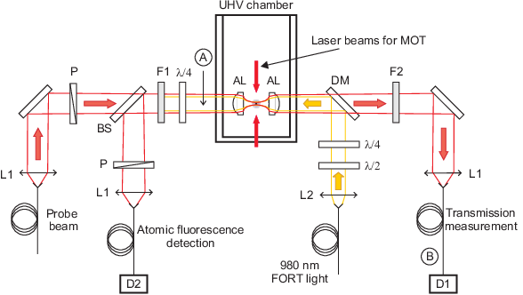
Two aspheric lenses ( mm) are mounted in a UHV chamber in a confocal arrangement. A single 87Rb atom is localized in a far-off resonant dipole trap (FORT) that is formed by 980 nm light at the focus of the lens pair. A probe beam is delivered from a single-mode fiber and focused onto the atom by one lens, and picked up by the other one. The confocal arrangement ensures that all of the incident probe power is collected in the absence of an atom, thus implementing the scheme discussed in the previous section. We use a circularly polarized probe to optically pump the atom into a closed cycling transition. After allowing some time for optical pumping, we measure the transmission of the probe beam that is defined as the ratio of count rates at detector D1 when the atom is present in the trap, to the count rate when the atom is absent. Such a measurement is carried out for different probe frequencies to obtain the transmission spectrum of a single Rb atom. The spectrum is fitted to a Lorentzian with the resonant frequency, the full width at half maximum (FWHM) of the spectrum and its minimum value on resonance as parameters. We obtained spectra for four different input waists of the probe, thus measuring extinctions for different focusing strengths. The observed FWHM never exceed 7.7 MHz, which is close to the natural linewidth of the optical transition (6 MHz), so we conclude that the atom was successfully kept in a two-level system. For each probe frequency, the probe power was adjusted such that the atom scatters 2500 photons per second, way below saturation. The properties of various transmission spectra obtained with different probe incident waists are summarized in Table 1.
| (mm) | (m) | m) | (%) | W (MHz) | |||
|---|---|---|---|---|---|---|---|
| 0.5 | 0.11 | 2.23 | 2.0 | 2.38 0.03 | 7.1 0.2 | 0.0362 | 3.58 |
| 1.1 | 0.24 | 1.01 | 2.0 | 7.2 0.1 | 7.4 0.2 | 0.1606 | 15.41 |
| 1.3 | 0.29 | 0.86 | 1.4 | 9.8 0.2 | 7.5 0.2 | 0.2157 | 20.40 |
| 1.4 | 0.31 | 0.80 | 1.4 | 10.4 0.1 | 7.7 0.2 | 0.2449 | 22.99 |
We also carefully characterized the losses of the probe beam in its optical path to ensure that our measured extinctions are not exaggerated by interference artefacts that can happen when certain elements in the transmission path preferentially filter more probe than the scattered light [9]. From point A to point B in Figure 6 we measured 53–60% transmission without the atom in the trap. The losses are mostly determined by 21% loss through the uncoated UHV chamber walls and 17–24% loss due to the coupling into the single-mode fiber at the transmission measurement channel. The coupling loss into the fiber increases as the input waist of the probe beam increases. Almost all losses can be ascribed to reflections at optical surfaces, except for a 9–16% re-coupling loss into a single mode fiber due to mode mismatch. We are thus reasonably confident that our measurement is free from artefacts that may arise due to incomplete collection of the probe.

In Figure 7 we compare the extinctions obtained from the experiment with values predicted by Equation (56). Since the probe is recoupled into a single mode fiber for every experimental point using a different lens that matches the probe waist, and the coupling lens has a NA=0.55 (corresponding to ), we can safely neglect any clipping, and use Equation (56) for estimating the extinction.
Obviously the measured extinctions are smaller than those predicted, especially for a larger focusing strength. We see a few possible reasons for this discrepancy. Firstly, the lenses we used in the experiment may not be suffciently close to an ideal lens, since they were designed for a situation with an additional window in the focusing part, which we did not have in our experiment. Secondly, the interaction strength is significantly affected by the motion of the atom in the dipole trap. While we do not have an independent measure of the position fluctuation of the atom in the trap, measurements in a similar trap showed a temperature of the atom in the trap of around 100 K due to the overlapping MOT [24], slightly below the Doppler temperature of 143 K of Rubidium. With our trap frequencies of kHz in transverse and kHz in longitudinal direction, this results in position uncertainties of nm and nm, respectively. The scattering ratio gets reduced due to the presence of the atom in regions with a reduced excitation field, and due to the spatially dependent detuning in the optical dipole trap. In paraxial approximation, we find an approximate reduction of the scattering rate due to the lower average field of
| (58) |
which results in a reduction of 2% for mm to 23% for mm. The reduction in and therefore in in our regime is about proportional to the temperature, so a doubling of the temperature alone would explain the discrepancy between theory and experiment already. On the other hand, the contribution due to a spatial variation of the resonance frequency is less than 1%. Additionally, the presence of the atom away from the focal point reduces the efficiency of the optical pumping. However, the observed extinction ratios still exceed the prediction by the parabolic wave front model in [6].
The inset of Figure 7 extrapolates the extinction we could expect for much stronger focusing; as mentioned earlier, the maximal extinction should reach 92.6%; whether such lenses can be manufactured, however, remains an open question. We also depicted the reflectivity of the fiber-atom-fiber system, which should reach values strong enough to be detected in an experimental setup. Extinction and reflectivity don’t match in this configuration, which means that there is still a significant amount of light which is neither transmitted nor reflected back into the optical fiber. Such losses are unavoidable for the described coupling scheme, which still places the fiber-atom-fiber system in disadvantage to a atom-cavity system in terms of success probability of scattering into known modes. If it would be possible to achieve a better overlap of photonic modes with the dipole transition, such losses should be reduced.
7 Conclusion
We have demonstrated both theoretically and experimentally that a substantial coupling efficiency of a light beam to a single atom can be achieved by focusing a light beam with a lens. By modifying the model given in [6], we have constructed a focusing field compatible with Maxwell equations that is suitable for the strong focusing regime. High values for the extinction of light (up to 92%) by a two-level atom stationary at the focus under the assumptions of weak on-resonant coherent probe are predicted. Within the limitations of our current trap, our experimental results confirm the possibility of observing a substantial extinction already for relatively weak focusing.
The measured extinction depends on the particular collection configuration of an experimental setup. It is thus not a fixed quantity for a given incident field. As such, the scattering ratio as defined by Equation (6) is a better quantity to characterize the interaction strength between a weak coherent field and an atom in free space, even though it loses a simple physical interpretation in the strong focusing regime. These results may also be of interest for experiments with single molecules [8, 25] and quantum dots [26].
Acknowledgement
This work was partly supported by the National Research Foundation, the Ministry of Education, Singapore, and by FRC grant R-144-000-174-112. The authors would like to thank Gert Zumofen, Ilja Gerhardt, and Mark Dennis for helpful discussions. ZC acknowledges financial support from ASTAR Singapore.
Appendix A Power scattered by the atom in a coherent light field
We briefly repeat the results for light scattered by a two-level atom following [10]. The steady-state population of the excited state in a two-level atom exposed to a monochromatic field can be obtained from the optical Bloch equations:
| (59) |
Therein, is the radiative decay rate of the excited state,
| (60) |
and is the Rabi frequency for a vanishing detuning of the driving field with respect to the atomic transition frequency . Therein, is the electrical dipole moment of the atom.
The optical power scattered by this atom is simply the product of energy splitting, decay rate and population of the excited state:
| (61) |
For weak () on resonant () excitation, the scattered power becomes
| (62) |
for an excitation field amplitude at the location of the atom.
Appendix B Transformation of local polarization by the lens
To obtain the local polarization of the focusing field in Equation (14), we consider a point P before the lens and an incident light field with polarization
| (63) |
or in the cylindrical basis,
| (64) |
where and are two unit vectors along the radial and azimuthal directions respectively. The ideal lens leaves the azimuthal component unchanged but tilts the radial component such that the local polarization of the field right after the lens is perpendicular to the line FP in Figure 1 (F is the focus point), that is:
| (65) | |||||
where and .
Appendix C Decomposition of a field into modes with cylindrical symmetry
For completeness, directly following [6], we outline the main properties of the cylindrical modes , which form a complete orthogonal set to compose an electric field that satisfies the source-free Maxwell equations,
| (66) |
where the summation over is a short-hand notation for
| (67) |
and are arbitrary complex amplitudes. The modes are characterized by four indices , where is the wave vector modulus, the wave vector component in -direction, an integer-valued angular momentum index, and the helicity. The dimensionless mode functions in cylindrical coordinates given in [27] are
| (68) | |||||
where is the transverse part of the wave vector, are the two circular polarization vectors, and
| (69) |
with the -th order Bessel function. As we are interested in a monochromatic beam with a fixed value of propagating in the positive direction (), the set of mode indices is reduced to where, for convenience, is taken as a mode index instead of . Now, we introduce the notation
| (70) |
for a complete summation over all possible modes. For a fixed the modes are orthogonal with respect to the scalar product
| (71) |
where is a plane perpendicular to the axis. This scalar product can thus be used to find the amplitudes of the modes in an arbitrary electric field compatible with the Maxwell equations.
References
References
- [1] Cirac J I, Zoller P, Kimble H J and Mabuchi H 1997 Phys. Rev. Lett. 78 3221–27
- [2] Duan L M, Lukin M D, Cirac J I and Zoller P 2001 Nature 414 413–18
- [3] Savage S M, Braunstein S L and Walls D F 1990 Optics Letters 15 628–30
- [4] Rosenfeld W, Berner S, Volz J, Weber M, and Weinfurter H 2007 Phys. Rev. Lett. 98 050504
- [5] Sondermann M, Maiwald R, Konermann H, Lindlein N, Peschel U and Leuchs G 2007 Applied Physics B 89 489–92
- [6] van Enk S J and Kimble H J 2001 Physical Review A 63 023809
- [7] Wineland D J, Itano W M, Bergquist J C 1987 Optics Letters 12, 389
- [8] Gerhardt I, Wrigge G, Bushev P, Zumofen G, Agio M, Pfab R, and Sandoghdar V 2007 Phys. Rev. Lett. 98, 033601
- [9] Tey M K, Chen Z, Aljunid S A, Chng B, Huber F, Maslennikov G and Kurtsiefer C 2008 Nature Physics 4 924–27
- [10] Cohen-Tannoudji C, Grynberg G and Dupont-Roc J 1992 Atom-Photon Interactions: Basic Processes and Application (Wiley, New York)
- [11] Richards B and Wolf E 1959 Proceedings of the Royal Society A 253 358–79
- [12] van Enk S J and Nienhuis G 1992 Optics Communications 93 147–58
- [13] Beijersbergen M W, Allen L, van der Veen H E L O and Woerdman J P 1993 Optics Communications 96 123–32
- [14] Jackson J D 1975 Classical Electrodynamics (Wiley, New York), 2nd ed
- [15] Born M and Wolf E 1975 Principles of Optics (Pergamon, Oxford)
- [16] Bohren C 1983 American Journal of Physics 51, 323
- [17] Bassett I M 1986 Journal of Modern Optics 33 279–86
- [18] Paul H and Fisher R 1983 Soviet Physics Uspekhi 26, 923
- [19] Davis R C and Williams C C 2001 Journal of the Optical Society of America 18 1543
- [20] Zumofen G, Mojarad N M, Sandoghdar V, and Agio M 2008 Phys. Rev. Lett. 101 180404
- [21] C. F. Bohren and D. R. Huffman 1983 Absorption and Scattering of Light by Small Particles (Wiley, New York).
- [22] Sheppard C J R and Török P 1997 Journal of Modern Optics 44 803
- [23] Mojarad N M, Sandoghdar V, and Agio M 2008 Journal of the Optical Society of America B 25 651
- [24] Weber M, Volz J, Saucke K, Kurtsiefer C and Weinfurter H 2006, Physical Review A 73 043406
- [25] Wrigge G, Gerhardt I, Hwang J, Zumofen G and Sandoghdar V 2008 Nature Physics 4 60–66
- [26] Vamivakas A et al. 2007 Nano Letters 7 2892–96
- [27] van Enk S J and Nienhuis G 1994 Journal of Modern Optics 41 963–77