Quantum Hall effect in bilayer and multilayer graphenes with finite gate voltage

Introduction— Among numbers of unusual physical properties of graphene (atomically thin graphite),[1, 2] study of the anomalous integer quantum Hall effect (QHE) was crowned with dramatic success. The Hall conductivity (per valley and per spin) is quantized as $\sigma_{xy}=-\frac{e^{2}}{h}(n+1/2)$, $n=0,\pm 1,\pm 2,\cdots$ wheres $\sigma_{xy}=-\frac{e^{2}}{h}n$ for usual two-dimensional (2D) electron gas. The difference $1/2$ is explained theoretically, based on the 2D massless Dirac fermions where a Landau level is located at zero energy. [3, 4, 5, 6] Moreover, QHE in bilayer system has also been observed as $\sigma_{xy}=-\frac{e^{2}}{h}n$, $n=\pm 1,\pm 2,\cdots$.[1] The characteristic feature of this result is that the step of $\sigma_{xy}$ at the strong-magnetic-field limit is twice larger than other steps (see Fig. 1). This behavior was successfully explained by McCann and Fal’ko based on an effective Hamiltonian in $2\times 2$ matrix form.[7]

On the other hand, one of the special situations of graphene system which can not be realized in other Dirac fermion systems such as organic conductor $\alpha$-(BEDT-TTF)₂I₃[8] is that the Fermi energy is tunable parameter by the gate voltage. Although the theory by McCann and Fal’ko well describes QHE in sufficiently small Fermi-energy regions, their Hamiltonian is no longer valid when the gate voltage becomes greater than the energy gap between two bands, which is the same order of the interlayer hopping energy. This situation is recently realized experimentally.[9] For such cases, we need to discuss the QHE based on the Hamiltonian of the bilayer graphene in $4\times 4$ matrix form [eq. (1) below].

The bilayer Hamiltonian is also important to discuss multilayer systems. For the Bernal stacking structure (it is also called AB or staggered stacking, and about 80 % of natural graphite falls into this category), the Hamiltonian of an $N$-layer system given by $2N\times 2N$ matrix can be block diagonalized into effective bilayer systems and a monolayer if $N$ is odd.[10, 11, 12, 13] This decomposition is related to the Fourier modes of the wave function along the stacking direction.[11] In this paper, we discuss QHE of bilayer system with finite gate voltage based on the four band Hamiltonian (1), and also that of multilayer systems.

Eigenvalues and eigenstates— The Hamiltonian of the bilayer graphene in $4\times 4$ matrix form is given by

where $\pi_{\pm}\equiv\pi_{x}\pm{\rm i}\pi_{y}$ with $\bm{\pi}\equiv\bm{p}+e\bm{A}/c$ is the momentum operator in a magnetic field $\nabla\times\bm{A}=(0,0,B)$. $v$ and $t$ are the Fermi velocity and interlayer hopping energy, respectively. We have ignored the trigonal wrapping effect stems from the next-nearest-interlayer hopping for simplicity. For the system with zero-magnetic field ${\cal H}_{0}$, dispersion relation is $E_{\mu}(\bm{k})=s_{2}(\sqrt{t^{2}+(2v\hbar k)^{2}}+s_{1}t)/2$, where the label $\mu=(s_{1},s_{2})$ specifies the outer and the inner bands ($s_{1}=\pm 1$), and positive and negative ($s_{2}=\pm 1$) energies, respectively, so that $t$ corresponds to an energy gap between two bands. Since the commutation relation between the momentum operators in eq. (1) is $[\pi_{\pm},\pi_{\mp}]=\mp 2eB\hbar/c$, there are correspondences with the creation and annihilation operators of the harmonic oscillator: $\pi_{\pm}\to\sqrt{2}\frac{\hbar}{l}a^{{\dagger}}$ $\pi_{\mp}\to\sqrt{2}\frac{\hbar}{l}a$ for $eB\gtrless 0$, where $l\equiv\sqrt{c\hbar/|eB|}$. Assuming that the wave function is given by linear combination of the number states of the harmonic oscillator $|n\rangle$, we obtain eigenvalues and eigenstates of eq. (1) as follows: The eigenvalues are

where $r\equiv\frac{l}{\sqrt{2}\hbar v}t$. For $n\geq 0$ with $\lambda\neq 0$, the eigenstates are given by

The zero-energy state ($\lambda=0$) is doubly degenerate. For these states, we specify the quantum numbers $n=0$ and $\mu$ as follows,

For large interlayer hopping $r^{2}\gg 1$, using the Taylor expansion, the inner band $s_{1}=-1$ is approximated as

This is consistent with the result obtained by McCann and Fal’ko.[7] Since the obtained eigenstates are given by number states like the nonrelativistic free fermion system, the degeneracy of each Landau level is also discussed in the same way that this is given by multiplicity of center of the coordinate: $V/2\pi l^{2}$ with $V$ being volume of the system.

Susceptibility— Before discussing the transport properties, we derive the magnetic susceptibility based on the the finite-magnetic-field formalism to check the consistency with other formalisms. In fact, the Hamiltonian (1) was introduced two decades ago by Safran motivated by graphite intercalation compounds.[14] He calculated magnetic susceptibility based on the weak-magnetic field formalism. An extention of this result with impurity scattering $\Gamma=\hbar/2\tau$ with $\tau$ being the collision time of quasiparticles is given by[12]

where $f(x)\equiv({\rm e}^{\beta(x-\mu)}+1)^{-1}$ is the Fermi distribution function with $\beta\equiv 1/k_{\rm B}T$ being inverse temperature. As discussed by Safran, in $\Gamma\to 0$ limit, the first term of the r.h.s of eq. (6b) gives diamagnetic logarithmic divergence near the zero Fermi energy $|\mu|\to 0$, while the second term gives paramagnetic behavior around $|\mu|\sim t$. Now let us calculate the magnetic susceptibility by the Landau quantization formalism. According to the functional integral method, the thermodynamic potential is given by

Here $\tilde{\omega}_{n}$ is Matsubara frequency of fermion including the chemical potential $\mu$ and effect of impurity scattering $\Gamma$ as ${\rm i}\tilde{\omega}_{n}={\rm i}\omega_{n}+[\mu+{\rm i}\ {\rm sgn}(\omega_{n})\Gamma]/\hbar$. Applying the Euler-Maclaurin formula

to the second derivative of eq. (7): $\chi=-\frac{1}{V}\left.\frac{\partial^{2}\Omega}{\partial B^{2}}\right|_{B=0}$, the first (second) term of the r.h.s of eq. (8) gives the first (second) term of the r.h.s of eq. (6b). Thus the result of this calculation coincides with that of the weak-magnetic field formalism.

Conductivity— The conductivity is given by the Kubo formula as,

where $\tilde{\Pi}_{ij}(\Omega)\equiv\Pi_{ij}(\Omega)-\Pi_{ij}(0)$ with $\{i,j\}\in\{x,y\}$. The polarization function $\Pi_{ij}(\Omega)$ is given by the current-current correlation function, and obtained as the analytical continuation of the Matsubara form:

where the matrix $\gamma_{i}$ is defined by $\bm{\gamma}\equiv\nabla_{\bm{k}}{\cal H}_{0}/\hbar$, and $\tilde{E}_{k}^{\mu}\equiv E_{k}^{\mu}/\hbar$. ${\rm i}\nu_{m}$ is Matsubara frequency of boson. We have ignored vertex corrections. After calculating the Matsubara frequency sums, and matrix elements $\langle\langle\cdots\rangle\rangle\langle\langle\cdots\rangle\rangle$ based on their symmetric (antisymmetric) properties for $\sigma_{xx}$ ($\sigma_{xy}$), the general expression of the conductivity (per valley and per spin) is obtained in the unified form as

Here the matrix elements between Landau levels $k$ and $k+1$ remain for $k\geq 1$, but other elements involving $k=0$ states are complicated due to the degeneracy of zero energy state. We have defined

and evaluated it analytically.

Quantum Hall effect— For clean system $\Gamma=0$ and dc limit $\Omega\to 0$, $X_{k,l}^{\mu,\nu}=[f(E_{k}^{\mu})-f(E_{l}^{\nu})]/(\tilde{E}_{k}^{\mu}-\tilde{E}_{l}^{\nu})^{2}$. Then after straightforward calculations of eq. (11), expression of the Hall conductivity becomes a simple form,

Here, we have defined $\tilde{f}(x)\equiv f(x)-1/2$. In this derivation it is important to keep the formula to satisfy the particle-hole symmetry.[4, 5] Moreover, assuming zero temperature and positive Fermi energy $\mu>0$, we have

where $[x]_{G}$ means the integer part of $x$, and we have defined $\tilde{B}\equiv\hbar v^{2}eB/c$. The first and the second terms of eq. (15) correspond to contribution from the inner ($s_{1}=-1$) and that from the outer ($s_{1}=+1$) bands, respectively. As expected, the Hall conductivity is quantized as a unit of $e^{2}/h$, reflecting that it is a topological number. Although, for the real QHE, the Anderson localization due to the impurity scattering is essential, the present calculation with $\Gamma=0$ is useful to estimate possible step structures of $\sigma_{xy}$.

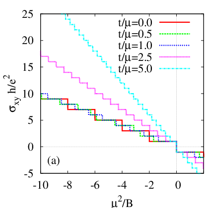
Results— The Hall conductivity $\sigma_{xy}$ with $\Gamma=0$ versus inverse magnetic field $1/B$ at zero temperature [eq. (15)] is shown in Fig. 2(a). Although the tunable parameter by gate voltage is $\mu$ rather than $t$ in experiment, we have shown the data as fixed $t$ for later convenience. The results show clear crossover behavior from two independent monolayer like regime to strongly coupled bilayer regime as the ratio of $t/\mu$ is changed. Similar structures of $\sigma_{xy}$ with inhomogeneous steps is also suggested to appear in monolayer system with interaction between different $K$ points. [15] In these data, we find that the slope of the Hall conductivity with respect to $\mu^{2}/B$ changes for $|t/\mu|>1$. This phenomenon is explained by rewriting inside of $[\cdots]_{G}$ in eq. (15) as

In r.h.s of eq. (16), $(\cdots)$ is $1+O(|t/\mu|)$ for $|t/\mu|<1$, which means that the slope of conductivity is proportional to $\mu^{2}/\tilde{B}$. On the other hand, for $t/\mu>1$, the energy band related to the QHE is only the inner band ($s_{1}=-1$), and $(\cdots)$ becomes larger than $1$ which means that the Landau levels strongly depend on the interlayer hopping $t$.

Next, in Fig. 3, we show $1/B$ dependence of the diagonal $\sigma_{xx}$ and the off-diagonal $\sigma_{xy}$ conductivities with impurity scattering $\Gamma=0.01\mu$. We have calculated dc limit of eq. (11) analytically, except for summation over the Landau levels. In principle, this summation can also be performed analytically using the Poisson formula.[16] We find dip structure in the steps in the region $|\sigma_{xy}|\gtrsim 5e^{2}/h$. The reason for this phenomenon is considered that the expression of $\sigma_{xy}$ implies that of $\sigma_{xx}$, and contribution of $\sigma_{xx}$ becomes large as the magnetic field is decreased. Actually, in the classical result for nonrelativistic free fermions, the expression is $\sigma_{xy}=-nec+\frac{1}{\omega_{\rm c}\tau}\sigma_{xx}$ where $n$ and $\omega_{\rm c}\propto eB$ are the electron density and the cyclotron frequency, respectively. This relation is also obtained in the analytical expression of the quantum case of 2D free fermions with constant $\Gamma$.[16]

Finally, we consider multilayer systems. Since Hamiltonians of multilayer systems with Bernal stacking are known to be decomposed into $[N/2]_{G}$ bilayer systems with effective hopping $t^{*}=t\sin\frac{m\pi}{2(N+1)}$ [$m=-(N-1),-(N-3),\cdots,N-1$], and a monolayer if $N$ is odd,[10, 11, 12, 13] the Hall conductivity can be calculated combining the above results. For example, the Hall conductivity with $\Gamma=0$ of $N$-layer system ($N=1$-$5$) obtained by eq. (15) and this matrix decomposition technique with $t/\mu=0.5$ is shown in Fig. 2(b). Although QHE of multilayer systems with general closed packed stacking structure where Bernal and rhombohedral stacking are mixed is discussed by Min and MacDonald using the matrix decomposition technique and the $2\times 2$ effective Hamiltonians,[13] their results are limited to the small gate voltage regions where only the inner band contributes to $\sigma_{xy}$.

Summary— We have discussed physical properties of bilayer graphene in finite magnetic field and finite gate voltage based on the Hamiltonian with four energy bands. We have checked the consistency between the weak- and the finite-magnetic field formalisms calculating the magnetic susceptibility. Then general formula of conductivity in this systems has been obtained. We have observed crossover of integer quantum Hall effect from two independent monolayer system to strongly coupled bilayer systems by changing the ratio of interlayer hopping energy and the gate voltage.

Acknowledgments— The authors are grateful to M. Oshikawa for discussion. M. N. thanks R. Shirasaki, A. Endo, N. Hatano, and H. Nakamura for discussion about their works.[16]

After this paper has almost been completed, we became aware of the paper by M. Koshino and T. Ando, Phys. Rev. B 77, 115313 (2008), which uses the same $4\times 4$ Hamiltonian as ours to discuss the optical properties at zero gate voltage.

References

- [1] K. S. Novoselov, A. K. Geim, S. V. Morozov, D. Jiang, M. I. Katsnelson, I. V. Grigorieva, S. V. Dubonos, and A. A. Firsov, Nature (London) 438, 197 (2005).
- [2] Y. Zhang, Y.-W. Tan, H. L. Stormer, and P. Kim, Nature (London) 438, 201 (2005).
- [3] Y. Zheng and T. Ando, Phys. Rev. B 65, 245420 (2002).
- [4] V. P. Gusynin and S. G. Sharapov, Phys. Rev. Lett. 95, 146801 (2005).
- [5] V. P. Gusynin and S. G. Sharapov, Phys. Rev. B 73, 245411 (2006).
- [6] N. M. R. Peres, F. Guinea, and A. H. Castro Neto, Phys. Rev. B 73, 125411 (2006).
- [7] E. McCann and V. I. Fal’ko, Phys. Rev. Lett. 96, 086805 (2006).
- [8] S. Katayama, A. Kobayashi, and Y. Suzumura, J. Phys. Soc. Jpn 75, 054705 (2006).
- [9] E. A. Henriksen, Z. Jiang, L.-C. Tung, M. E. Schwartz, M. Takita, Y.-J. Wang, P. Kim, and H. L. Stormer, Phys. Rev. Lett. 100, 087403 (2008).
- [10] F. Guinea, A. H. Castro Neto, and N. M. R. Peres, Phys. Rev. B 73, 245426 (2006).
- [11] M. Koshino and T. Ando, Phys. Rev. B 76, 085425 (2007).
- [12] M. Nakamura and L. Hirasawa, Phys. Rev. B 77, 045429 (2008).
- [13] H. Min and A.H. MacDonald, Phys. Rev. B 77, 155416 (2008).
- [14] S. A. Safran, Phys. Rev. B 30, 421 (1984).
- [15] P. M. Ostrovsky, I. V. Gornyi, and A. D. Mirlin, arXiv:0712.0597.
- [16] R. Shirasaki, A. Endo, N. Hatano, and H. Nakamura, unpublished.