Numerical simulations of rotating axisymmetric sunspots
Abstract
A numerical model of axisymmetric convection in the presence of a vertical magnetic flux bundle and rotation about the axis is presented. The model contains a compressible plasma described by the nonlinear MHD equations, with density and temperature gradients simulating the upper layer of the sun’s convection zone. The solutions exhibit a central magnetic flux tube in a cylindrical numerical domain, with convection cells forming collar flows around the tube. When the numerical domain is rotated with a constant angular velocity, the plasma forms a Rankine vortex, with the plasma rotating as a rigid body where the magnetic field is strong, as in the flux tube, while experiencing sheared azimuthal flow in the surrounding convection cells, forming a free vortex. As a result, the azimuthal velocity component has its maximum value close to the outer edge of the flux tube. The azimuthal flow inside the magnetic flux tube and the vortex flow are prograde relative to the rotating cylindrical reference frame. A retrograde flow appears at the outer wall. The most significant convection cell outside the flux tube is the location for the maximum value of the azimuthal magnetic field component. The azimuthal flow and magnetic structure are not generated spontaneously, but decay exponentially in the absence of any imposed rotation of the cylindrical domain.
Keywords:
MHD — convection — Sun: magnetic fields — sunspots1 Introduction
Observations of sunspots rotating around their own axis, which is perpendicular to the plane of the photosphere, have a long history throughout the twentieth century. Hale (1908) and Evershed (1910) noticed the rotation as well as a vortex forming around the rotating sunspot. Observations in the photosphere and corona continued through the century, culminating in the high resolution measurements of today. (See Brown et al. (2003) and references therein.) An exciting development during the last decade has been the ability to measure the associated flow beneath the photosphere (Gizon & Birch, 2005; Zhao & Kosovichev, 2003).
There is a distinct radial profile associated with the azimuthal velocity of rotating sunspots. Brown et al. (2003) found that the umbra (in which the rotation axis resides) has small average azimuthal velocities, while the fastest rotation occurs at some point along the radial length of the penumbra. The rotation then tails away to a negligible value outside of the sunspot. The peak azimuthal velocity in the penumbra can be more than double that inside the umbra. Brown et al. (2003) found suggestions of rotation outside some sunspots, but these observations are hampered by an ambiguous penumbral edge. In contrast, Yan & Qu (2007) observed a rotating sunspot where the maximum azimuthal velocity occurred inside the umbra. The rotation persisted in the penumbra and the area near the penumbra, with the angular velocity reducing as one moves radially away from the umbra. The surrounding area far removed from the penumbra experienced a slow rotation in the opposite direction from that of the rotating sunspot.
It is not clear if the direction of rotation has a hemispheric preference. Knoška (1975), and references therein, found that the majority of rotating sunspots in both hemispheres turn anticlockwise. However, Ding, Hong & Wang (1987) found a preference, with clockwise (anticlockwise) rotation predominantly in the southern (northern) hemisphere. This would suggest that the Sun’s differential rotation associated with the global flow field has an influence. The Coriolis force due to the Evershed flow field would cause rotation in the opposite direction. However, helioseismic observations (Gizon & Birch, 2005), supported by numerical results (Hurlburt & Rucklidge, 2000; Botha, Rucklidge & Hurlburt, 2006), show a converging horizontal flow below the Evershed flow, which leads to cyclonic vorticity and hence a possible contribution from the Coriolis force.
The small sample of rotating sunspots studied by Brown et al. (2003) suggests that younger sunspots rotate faster than older ones. However, it was difficult to judge the ages of the sunspots in the sample. The rotation rates are time dependent, with all rotation eventually decreasing with time. The peak rotation in the penumbra can be anything up to 3 degrees per hour, as observed by Brown et al. (2003). The same time evolution was observed in a rotating pore (Dorotovič et al., 2002). This behaviour suggest that some of the rotation are caused by local events that are transitory in nature. This conclusion is strengthened by an observation of damped oscillatory motion, which had a maximum rotation of 3.5 degrees per hour (Kučera, 1982).
A possible mechanism causing rotating sunspots is the rise of twisted flux ropes (Gibson et al., 2004). In this model the rotation of two flux rope poles is observed after the central horizontal portion of the flux rope has emerged through the photosphere. This implies the existence of two co-evolving sunspots of opposite magnetic polarity. This is generally not in evidence in the observations, mostly because leading sunspots are often followed by a more diffuse opposite polarity.
It was shown by Gopasyuk & Gopasyuk (2005) that when the averaged velocity and magnetic field components are subtracted from observed sunspots, the result fits a lightly damped sinusoidal wave. This implies that as well as the motion described so far, sunspots also experience torsional oscillations. Using the thin flux tube model, Musielak et al. (2007) found that in a compressible, isothermal field-free medium, linear torsional Alfvén waves along the magnetic tube do not have a cutoff frequency.
The rotation of sunspots has been linked to the formation of soft X-ray sigmoids as well as the eruption of flares (Alexander, 2006; Régnier & Canfield, 2006; Tian & Alexander, 2006). Numerical simulations by Gerrard et al. (2003) show that by adding a horizontal photospheric flow to the rotation, the generation of flares is enhanced as both rotation and flow increase the complexity of the magnetic field. This is supported by the observation that flare activity is correlated to magnetic flux and kinetic vorticity (Mason et al., 2006).
Evidence from helioseismic measurements show that the rotation of sunspots, as observed in the photosphere, extends into the deeper layers of the sun. Up to a depth of approximately 7 Mm vortical flow in the same direction as the rotation of the sunspot exists, while below 7 Mm a vortical flow opposite to the sunspot rotation direction is observed (Kosovichev, 2002; Zhao & Kosovichev, 2003; Gizon & Birch, 2005). However, it should be noted that helioseismic measurements are difficult and not always consistent. For example, up to a depth of 3 Mm a converging inflow is found when using p modes, while f mode measurements find only outflows down to 10 Mm (Gizon & Birch, 2005).
In this paper an axisymmetric model is used to simulate rotation around a central magnetic flux bundle. The values of the physical parameters of the model are chosen to describe the solar convection zone from a depth of approximately 500 km below the visible surface of the Sun to a depth of approximately 6000 km (Botha, Rucklidge & Hurlburt, 2006). The numerical domain is a cylinder with an aspect ratio of , i.e. one unit deep and a radial distance of three units. This implies that we are simulating magnetoconvection on the supergranular scale. To generate azimuthal flow and magnetic field, the whole domain is rotated at a constant angular velocity. Strictly speaking this is not equivalent to simulating a pore or sunspot where only the magnetic flux bundle rotates. However, in spite of driving the azimuthal flow throughout the numerical domain, we find that the solution tends to conform to observations of Brown et al. (2003), where a maximum azimuthal flow occurs close to the magnetic flux bundle. This means that a vortical flow forms around the flux bundle while the plasma inside the bundle rotates as a solid body. This type of flow is formally described as a Rankine vortex.
Our numerical results may be compared to results found by Jones & Galloway (1993), who studied a Boussinesq fluid in an axisymmetric cylinder. They imposed two types of boundary conditions: a stress-free outer wall as well as an external flow, implemented by rotating the outer wall of the fixed cylinder. A flux bundle formed at the central axis, with the maximum angular velocity occurring near the axis. For high magnetic field strength, described by the dimensionless Chandrasekhar number (), the flux bundle broadened with the stress-free boundary conditions producing a reverse in azimuthal magnetic flux near the axis, while the imposed external flow produced a reverse azimuthal flow near the axis. The reversal in the azimuthal magnetic field is ascribed to the conservation of angular momentum under stress-free conditions, while the flow reversal obtained with the imposed external flow is ascribed to the working of the Lorentz force.
In Section 2 the mathematical model and its numerical implementation is described. This is followed by the numerical results. When no rotation of the numerical domain is present (Section 3.1), no azimuthal velocity and magnetic field are generated spontaneously: both quantities are small and decay exponentially with time. This case is useful to compare the rotating solutions against. Driven by the rotating numerical domain, the solution settles into a time independent solution that shows rigid rotation of the plasma in the magnetic flux tube and vortical rotation around it (Sections 3.2 and 3.3). This solution is robust and essentially stays the same when the magnetic field strength is increased (Section 3.4), the Prandtl number is lowered (Section 3.5), as well as when the stratification is increased (Section 3.7). The latter part of the numerical investigation explores the influence of the numerical domain on the solution. This we do by changing the bottom and outside boundary conditions (Sections 3.6 and 3.8). We conclude the paper with a summary of the results.
2 Model
Partial differential equations describing compressible magnetoconvection are solved in an axisymmetric cylindrical geometry, using a numerical code developed for this purpose. A detailed description of the two dimensional (2D) model is given by Hurlburt & Rucklidge (2000). Here we extend the model to 2.5D by including azimuthal components in addition to the radial and axial components. A constant angular velocity is added that introduces the Coriolis and centrifugal forces into the Navier-Stokes equation.
2.1 Mathematical model
The initial temperature and density profiles in the vertical () direction are given by
| (1) | |||||
| (2) |
The temperature and density are scaled so that they are equal to 1 at the top of the static atmosphere. The initial temperature gradient is given by , while is the polytropic index. The equations for fully compressible, nonlinear axisymmetric magnetoconvection that we use are
| (3) | |||||
| (4) | |||||
| (5) | |||||
| (6) | |||||
| (7) |
The cylindrical reference frame is rotated about its axis at a constant angular velocity of , which is responsible for the Coriolis and centrifugal terms in the Navier-Stokes equation (4). The vector potential gives the and components of the magnetic field while the azimuthal component is included explicitly, so that the magnetic field is given by
| (8) |
The velocity consists of three components, namely , where refers to the azimuthal velocity relative to the rotating reference frame. We also use the auxiliary equations
| (9) |
and the following notation: is the ratio of specific heats; the Prandtl number; the magnetic diffusivity ratio at ; and the Chandrasekhar number given by
| (10) |
where is the depth of the domain, the magnetic permeability, the magnetic diffusivity and the kinetic viscosity. The rate of strain tensor is given by
| (11) |
while the dimensionless thermal conductivity is related to the Rayleigh number in the following way:
| (12) |
is a measure of the importance of buoyancy forces compared to viscous forces in the middle of the layer, and is used to drive the convection in the model. The addition of rotation adds an additional scaling which relates the convective timescale to the rotational timescale. Following Gilman (1977) we express this ratio using the convective Rossby number defined as
| (13) |
Brummell, Hurlburt & Toomre (1996) found that this parameter, which can be evaluated from the control parameters, is typically close to that based on the traditional definition of the Rossby number, namely the ratio of the rms vorticity of the flow to the vorticity associated with the rotating cylinder. The effects of rotation are significant for , and dominate for . For supergranules and sunspot moats, .
All the other symbols have their usual meaning. The physical quantities are dimensionless, with the length scaled proportional to the depth of the numerical domain, velocity scaled proportional to the sound speed at the top of the domain and temperature, magnetic field, density, and pressure all scaled proportional to their initial values at the top of the numerical domain. These top initial values are radially uniform and do not change throughout this paper, as discussed in Section 2.2.
2.2 Numerical implementation
The computational domain is an axisymmetric cylinder of radius , situated in the plane so that
| (14) |
with at the top of the box (Hurlburt & Rucklidge, 2000; Botha, Rucklidge & Hurlburt, 2006). We require that all variables be sufficiently well-behaved at the axis () and that the differential operators in the PDEs are non-singular. This implies that
| (15) |
Terms like , and are evaluated using l’Hôpital’s rule, while terms containing cancel algebraically.
The outside wall () is a slippery, impenetrable wall with no lateral heat flux across it (i.e. an insulator):
| (16) |
The magnetic potential has the value at the outside wall, which was chosen so that the initial vertical uniform field satisfies .
At the bottom boundary the magnetic field is vertical. The temperature is chosen to be constant with value from equation (1). The bottom boundary is impenetrable and stress free, i.e.
| (17) |
The top of the box is treated as impenetrable for the plasma, with a radiative temperature boundary condition given by Stefan’s law:
| (18) |
The in Stefan’s law is the same as in (1), so that the equilibrium profile used as initial condition is not destroyed. The Stefan-Boltzmann constant will enter (18) only when we dimensionalize it. The magnetic field is matched to a potential field on top of the numerical domain, , where is a linear operator, so that and are continuous across the boundary. The potential field is solved by assuming an infinitely tall conducting cylinder of radius above the domain, with the magnetic field becoming uniform as . A more detailed description is given by Hurlburt & Rucklidge (2000). No currents exist inside the potential field and consequently we choose along the top of the box. From (15) it then follows that along the top boundary.
One consequence of these boundary conditions is that no current escapes from the numerical domain: on and on and 1. It follows that the boundaries do not provide any net vertical torques, and so do not contribute to changes in the vertical component of the total angular momentum, . Nonetheless, is not conserved in compressible convection: the Coriolis term can lead to changes in , for example, when mass is transported to larger distances from the axis. (Note that this does not occur in incompressible convection.) A consequence of this is that as the solution evolves through time, tends to drift, making the meaning of the parameter less precise. Therefore, we will look for steady solutions with no net vertical angular momentum relative to the rotating frame. We achieve this by calculating the drift in the value of after each iteration and then introducing a correction in the form of an equivalent rigid body rotation in the opposite direction. This alters the evolution of the PDEs (slightly), but steady states are correct solutions of the PDEs. In our oscillatory solutions we remove the constraint from and follow its time evolution. This is discussed in Section 3.9.
A uniform, vertical magnetic field is used as initial condition. For a nonrotating cylinder () the azimuthal magnetic field is perturbed (Section 3.1). For a finite angular velocity () the evolution of the plasma is triggered by starting the quiet, nonrotating plasma with a finite and no plasma perturbation. Both these initialisations ensure that at the start of the numerical simulations.

The density does not in principle satisfy a boundary condition, but we impose the value of the normal derivative of obtained from the Navier-Stokes equation (4).
The numerical code was developed specifically for this type of calculation (Hurlburt & Rucklidge, 2000). Sixth-order compact finite differencing is used, which reduces at the boundaries to fifth-order accuracy for first-order derivatives and fourth-order accuracy for second-order derivatives. The grid intervals were chosen to be equal in the and directions, with 240 grid points in the horizontal and 80 in the vertical for the majority of calculations. The time evolution obtained fourth-order accuracy through a modified (explicit) Bulirsch-Stoer integration scheme, with the time step limited by the Courant condition (using the maximum sound and Alfvén speeds, as well as the thermal diffusive limit), multiplied by a safety factor of 0.5.




3 Numerical results
Unless otherwise stated, the results shown here have been obtained with the following parameter values: , , , , , , and . The results are presented in the format given in Figure 1.
3.1 No rotation
When no is rotation present ( or ), the azimuthal magnetic field is perturbed initially and the plasma is allowed to evolve through time. The solution reaches the state depicted in Figure 2, with the explanation of the diagnostic given by the left hand box in Figure 1. The solution described here is typical of the plasma state when the axisymmetric cylinder is not rotated (Hurlburt & Rucklidge, 2000; Botha, Rucklidge & Hurlburt, 2006) and it provides a convenient base against which to compare results obtained with rotation.
From an initial vertical magnetic field, the convection sweeps the magnetic field towards the central axis where it forms a flux tube. A large anticlockwise convection cell forms next to the tube, flowing towards the flux tube at the top of the numerical domain. This flow direction keeps the magnetic field confined to the central axis. The temperature is time dependent in that a cold plasma blob forms at the top next to the magnetic flux tube, is convected down the side of the tube, only to dissipate as it is convected along the bottom boundary. Figure 2 shows a new cold plasma blob forming at the top while the remnants of the previous cold blob is still visible at the bottom, moving towards the outer boundary. This temperature oscillation has a period of approximately 1.275 time units, which corresponds roughly to half the circulation time around the convection cell. The upper layers of the plasma are heated by the upflow next to the outer boundary and the resulting hot plasma blob is time independent. The azimuthal current density has its maximum value (in both directions) next to the flux tube where the magnetic field gradient is the highest. Azimuthal flow and magnetic structure are not generated spontaneously. The azimuthal components, generated by the initial perturbation, are small and decay exponentially as the solution evolves through time.
Periodic oscillations, an example of which is the time dependent temperature next to the magnetic flux bundle, are familiar from Rayleigh-Benard convection (Clever & Busse, 1995). Jones & Galloway (1993) found periodic oscillations for a Boussinesq fluid in an axisymmetric cylinder. As must be expected, as in our case they found no spontaneous generation of azimuthal velocity or magnetic field components.
Given the model’s temperature and density profiles in (1) and (2), the sound speed increases and the Alfvén speed decreases with depth. The inflowing layer at the top of the box is deeper than the outflowing layer at the bottom. This is ascribed to the fact that the total radial momentum in the system is zero. The higher density at the bottom leads to a shallower outflowing layer with lower radial velocities transporting the same momentum outwards as what the deeper top layer with higher velocities transports inwards. The simulation runs with a maximum Mach number of approximately 1. The time step is limited by the thermal diffusivity, with the dimensionless thermal conductivity calculated using (12). This constraint on the time step is true for all the numerical simulations in this paper.
3.2 Introduce rotation
By introducing a constant angular velocity of () we obtain the solution in Figure 3. The one convection cell in the case of no rotation (Figure 2) has split into two cells, i.e. a finite reduces the characteristic wavelength of the convection in the radial direction. This effect of rotation on convection is well known (Chandrasekhar, 1961). The convection cell next to the flux tube always has an anticlockwise flow direction with an inward flow at the top, so that it forms a collar which forces the magnetic field together at the central axis (Botha, Rucklidge & Hurlburt, 2006).
By introducing a finite , the centrifugal term in equation (4) provides a force in the radial direction. This manifests as a change in density contours, which go from being approximately horizontal without rotation (Figure 2) to being slanted at the outer wall (Figure 3). This boundary effect is localized and does not affect the solution in the domain interior. The treatment of the outer boundary is discussed in more detail in Section 3.8.
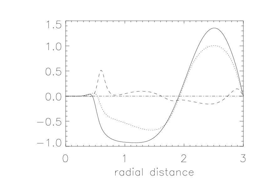
There is no time dependence in the solution. The radial profiles of the velocities are given in Figures 4 to 6 at three depths. All three velocity components are of the same order of magnitude. The radial velocity (Figure 4) shows the two cells circulating in opposite directions, as well as the fact that the speed is higher in the upper part of the numerical domain.
The azimuthal velocity (Figure 5) shows that the plasma inside the strong magnetic field of the flux tube rotates as a solid body, with maximum rotation on the outside edge of the tube. In the convection area of the solution the rotation is in the form of a vortex with the azimuthal velocity gradually falling away with radius. This rotation pattern is uniform throughout the depth of the box and compares well with observations that show the largest azimuthal velocities are located in the penumbra (Brown et al., 2003). One can fit the profile with a Rankine vortex, described by
| (19) |
with the magnetic flux tube radius and . An observer in the rotating reference frame of the cylinder will measure an azimuthal velocity profile of
| (20) |
The values of and measured for are presented in Table 1 and the radial profile of in Figure 8. Rankine vortices are used regularly to model tropical cyclones on Earth. Helioseismic measurements of flow around sunspots in the upper convection zone show a strong resemblance to the flow of hurricanes on Earth (Zhao & Kosovichev, 2003). It is a happy coincidence that Herschel thought of sunspots as large cyclonic storms (Thomas & Weiss, 1992). In our model the Rankine vortex makes physical sense. Convection is suppressed where the magnetic field is strong. The radial dependence of the azimuthal velocity in these regions is that of a rotating rigid body. Since the region experiencing rigid rotation corresponds to the magnetized region in all cases, we deduce that magnetic effects are responsible for the rigid body rotation. A vortex exists around the flux tube. Angular momentum mixes in axisymmetric convection, which results in the free vortex in the field-free convection cells where convection is strong. The counter flow near the outer wall is a consequence of the treatment of in our solution. Since our solution has zero vertical angular momentum relative to the rotating reference frame, a significant counter flow has to occur at the edge in order to balance the peak flow next to the flux tube.
The vertical velocity (Figure 6) shows the strong downflow at the outside of the magnetic flux tube and at the outer edge of the numerical domain, as well as the upflow between the two convection cells. Comparing the two downflows, we observe that the downflow at the outer edge is stronger than that next to the magnetic flux tube. It is essential to use a large enough aspect ratio () so that the outer boundary is removed from the physics around the magnetic flux tube. A appears to be a reasonable compromise between this and the computational limitations.
The radial and axial magnetic field components are concentrated in the magnetic flux tube, with three times larger than . Figure 7 shows the radial profile of , the size of which is an order of magnitude smaller than . is confined mainly to the inner convection cell next to the magnetic flux tube. The current, obtained from the magnetic field through equation (9), reflects the distribution of the magnetic field. Its azimuthal component is concentrated on the outside of the magnetic flux tube where the radial gradient in the magnetic field is the largest. The radial and vertical components are distributed in and around the inner convection cell around the azimuthal magnetic field maxima (Figure 3). At the top and bottom boundaries the radial current density has local maxima due to the fact that no current flows out of the box.

| (measured downward) | |||
|---|---|---|---|
| 0.1 | 0.25 | 0.75 | 0.55 |
| 0.5 | 0.69 | 0.55 | |
| 0.75 | 0.57 | 0.63 | |
| 0.2 | 0.25 | 1.16 | 0.68 |
| 0.5 | 1.09 | 0.68 | |
| 0.75 | 0.95 | 0.73 | |
| 0.3 | 0.25 | 1.27 | 0.85 |
| 0.5 | 1.24 | 0.84 | |
| 0.75 | 1.13 | 0.88 |
3.3 Increase rotation
The convective Rossby number () associated with the rotation around the central axis decreases as increases. The associated with the circulation around the convection cells for the case with , i.e. , compares well with that of supergranulation in the Sun. of larger values correspond to even larger-scale flows. In all cases the rotation rate is low enough that it should not significantly change the value of the critical Rayleigh number for the onset of convection (see Brummell, Hurlburt & Toomre (1996)) and thus the cases exhibit comparable amplitudes.
As the magnitude of increases, the width of the magnetic flux tube increases. Figure 9 shows a time independent solution with . The magnetic field strength inside the flux tube decreases with increasing width, allowing weak convection to form inside the flux tube itself. Figure 9 shows that the upflow in the flux tube heats the plasma in the top layers of the tube, while very weak outflow forms along the top boundary. Eventually, for , the convection inside the flux tube becomes strong enough to break it into concentric rings.
As rotation increases and with it the width of the magnetic flux tube, the magnetic field lines forming the flux tube straighten. This causes the azimuthal current density to decrease in both positive and negative azimuthal directions. The position of stays the same: it flows around the flux tube, created by large magnetic field gradients there.
Increasing also increases the size of the centrifugal force in equation (4). For the density contours inside the flux tube are approximately horizontal (Figure 3). For density contours become slanted, due to weak convection inside the flux tube as well as the centrifugal force acting on the plasma. As a result, there is a slight depletion of plasma at the top of the magnetic flux tube near the central axis, while the area of density variation along the inside edge of the flux tube increases. Figure 9 shows that inside the convection cells the increase in causes a slight depression of density contours.


The plasma rotates as a Rankine vortex for all values of . Where the magnetic field is strong enough to suppress convection, the flow is a forced vortex in the form of rigid body rotation, while in the field-free convection region we observe a free vortex. The dependence in the convection region corresponds to homogeneous angular momentum that is caused by the effective mixing by the convection. As the width of the magnetic flux tube increases with the increase in , the radius of the forced vortex also increases (Table 1). The radial profiles of for different values can be compared in Figures 5 and 10. They show that as increases, the maxima next to the magnetic flux tubes increase as well. (See also Table 1.) To maintain the initial , the counterflow at the outer wall increases in sympathy. This is in contrast to Jones & Galloway (1993), who found a retrograde flow at the central axis for large values in a Boussinesq fluid. To generate a retrograde flow near the central axis, we had to change the temperature boundary condition at the lower boundary in our model (Section 3.6). The rigid body rotation inside the magnetic flux tube is perturbed when the weak convection inside the tube becomes strong enough to influence the local magnetic field. Figure 9 shows the strength of the convection inside the flux tube, while Figure 10 shows the deviation from rigid body rotation. This deviation increases deeper in the numerical domain where convection is stronger.


The azimuthal magnetic field tends to be located in the convection cells closest to the central axis. In the case of this is in the collar flow around the flux bundle (Figure 3). For a small convection cell starts to form inside the flux bundle at its base, due to weak convection inside the flux bundle (Figure 9). As this cell grows in strength, the amplitude of located in it grows in strength relative to the in the collar flow outside the flux bundle. The directions of in the small cell inside the flux bundle and that of in the collar flow are anti-parallel. This corresponds to the direction of flow of the convection cell. Figure 9 shows that a clockwise convection cell has a pointing in the positive direction (i.e. into the page), while in an anticlockwise cell points in the negative direction (i.e. out of the page). This is caused by the interaction of the magnetic field with the velocity in the first term on the right hand side of equation (7). The current surrounding the local maxima of has the same direction as the local convection, since it is calculated using equation (9).
The behaviour when rotation is increased is summarized in Figure 11. As increases the magnetic flux tube widens and the field lines straighten and become more vertical, which leads to a decrease in the radial component of the magnetic field. At the same time the azimuthal velocity and magnetic field components increase, being driven by . Compared to these changes, the radial and axial velocity components stay relatively stable. All velocity components increase in absolute value as increases.
3.4 Increase magnetic field strength
From previous numerical studies it is known that an increase in the magnetic field increases the width of the magnetic flux tube for nonrotating solutions (Hurlburt & Rucklidge, 2000). This is also true when rotation is present, which can be seen when Figure 9 with and is compared with Figure 12 for and . The solution is time independent and the growth in flux tube width takes place at the expense of the radial dimensions of the convection cells.
The magnetic flux tube retains its configuration, with an anticlockwise convection cell holding the flux tube in place. The stronger magnetic field suppresses the weak convection inside the magnetic flux tube, which was present when (Figure 9).
As the area with strong magnetic field becomes wider, the field-free convective region is compressed. The decrease in the field-free area is accompanied by lower flow velocities of convection. Here the maximum Mach number of the solution is 0.8, while for . The maximum measured azimuthal velocity for (Figure 12) is also 2/3 of what it is for (Figure 9).
The weaker flow in the convection cell around the magnetic flux tube means the field lines are less compressed when compared to the case when (Figure 9). This leads to lower gradients at the flux tube’s edge, which in turn implies a lower azimuthal current density flowing around the flux tube, since is calculated using equation (9).
The azimuthal flow of this solution fits that of a Rankine vortex. By suppressing the weak convection inside the flux tube that is present for , the plasma flow inside the flux tube becomes more like rigid body rotation. (Compare Figures 10 and 13.) The maximum next to the flux bundle is lower for due to the lower levels of convection in the solution. This is also true for the counter flow at the outer wall.
The azimuthal magnetic field has its maximum in the convection cells closest to the central axis. In Figure 9 with , there exists a small clockwise cell at the base of the flux tube. This cell is strong enough to contain a significant part of , with the anticlockwise collar flow containing an anti-parallel component. Here, for (Figure 12), the small clockwise cell inside the flux tube is suppressed, so that is mainly located in the anticlockwise collar flow.


3.5 Lower Prandtl number
Decreasing the Prandtl number causes the convection described by the steady solution to become more vigorous, as can be seen when Figure 3 (with ) is compared to Figure 14 (with ). For the maximum Mach number in the solution is 0.9, while for we have . The lower value brings the simulation closer to the physical conditions in the upper convection zone. The dimensionless thermal conductivity , defined by (12), changes from for to for . For we have and with we have a convective Rossby number of .
For lower Prandtl numbers the inner convection cell increases its size at the expense of the width of the magnetic flux bundle, and to a lesser degree the width of the convection cell next to the outer boundary. Not only is the inner cell larger, but the velocity amplitudes have higher maximum values. However, the relative differences between the velocity components are independent of the value of , with the azimuthal component approximately a third the size of the radial and axial components. The azimuthal flow takes the form of a Rankine vortex (Figure 15). The rigid body rotation inside the flux bundle is faster than when (Figure 5), with a higher maximum next to the bundle. The flux bundle is also narrower, which means that to maintain the initial during the simulation, the counter flow at the outer boundary needs to be only slightly larger than when .
The stronger convection pushes the magnetic flux into a thinner flux bundle at the central axis, so that the strength of increases for lower values of . The size of relative to stays approximately the same for all values of . As in the case for (Figure 3), the azimuthal magnetic field is mostly located in the inner convection cell, with its maxima next to the magnetic flux bundle. The stronger convection also causes the curvature and gradients of the magnetic field lines in the plane to increase, which increases the size of the azimuthal current density obtained from equation (9). The position of stays the same.
The effects of the enhanced convection are visible in the density contours. For the density contours in the convection cells are approximately horizontal (Figure 3) while for significant variation in the radial direction occurs (Figure 14). At the central axis, where the convection is suppressed by the strong magnetic field, the contour lines stay approximately as they were with and its lower convection strengths.
There are changes in the temperature profile of the solution. The stronger upflow between the two convection cells leads to a larger variation from the original heat profile in the upper layers of the solution, as can be seen when in Figures 3 and 14 are compared. Also, for lower values the thermal diffusion rate becomes more significant, which reduces the radial extent of the heated plasma above the upflow.


| Lower boundary: constant | Lower boundary: constant | ||||
| max(Mach) | at | max(Mach) | range at | ||
| 0 | 1.0 | 1.2 | 11 | 0.6 | (9.34,10.19) |
| 0.1 | 1.0 | 0.9 | 11 | 0.6 | (9.33,10.42) |
| 0.1 | 0.3 | 1.7 | 11 | 1.1 | (9.05,10.43) |
| 0.1 | 0.1 | – | – | 1.3 | (8.59,10.20) |
3.6 Temperature prescription at bottom boundary
To determine the extent to which the bottom boundary is influencing the result, we changed the temperature prescription on this boundary from a constant value to a constant . From equation (1) we set , so that the heat flux stays equivalent to the heat flux for a constant boundary condition. A linear stability analysis by Hurlburt, Toomre & Massaguer (1984) determined that this change in boundary condition results in halving the critical Rayleigh number for the onset of convection, and hence one would expect somewhat more vigorous convection for the same Rayleigh number, all other aspects of the solution being equal. However, the numerical results discussed in this section show that for this highly nonlinear system, the change in the lower boundary condition leads to lower convection levels.
For low Prandtl numbers, such as in Figure 16, the basic configuration of two convection cells and a central magnetic flux tube remains as before. The radial profile of the azimuthal flow is that of a Rankine vortex. The strength of convection outside the magnetic flux tube is lower than for the bottom boundary condition of constant temperature, while the magnetic flux tube is wider with very weak convection inside it.
For Prandtl numbers of the solution changes into one convection cell that is outflowing at the top. This new flow direction does not provide an efficient collar to contain the magnetic flux (Botha, Rucklidge & Hurlburt, 2006), so that the magnetic field spreads out in the radial direction rather than being contained at the central axis. Under these circumstances it is possible to have horizontal magnetic field lines above the main convection cell. Figure 17 gives the solution for , while Figures 18 to 20 give the radial profiles of for various parameter values.


Figure 17 shows the solution with . A solution in the same parameter space but with constant temperature at the bottom boundary is given by Figure 3. When comparing the two solutions, it is clear that the level of convection is lower in the case of constant boundary condition. This is shown explicitly in Table 2: the maximum Mach number is lower when a constant is used. It also shows in the fact that the maximum azimuthal velocity is weaker in Figure 17 than in Figure 3. This is true for all choices of parameter values. The maximum Mach number in the solution increases as decreases, in line with the discussion in Section 3.5 and the fact that more heat flows through the system. In Table 2 the solution for and constant does not have a counterpart when a constant temperature boundary condition is used, because the convection becomes too vigorous and large shocks form that terminate the numerical simulation. This agrees with the conclusion that a constant at the lower boundary leads to lower convection levels.


The weaker convection allows the magnetic flux tube to be wider, so that the value of is lower. The different flow pattern when also contribute to the lower vertical magnetic component, in that the magnetic field now has a significant horizontal component (Figure 17). Another consequence of the weaker convection is lower magnetic field gradients in the plane. This leads to lower levels of azimuthal current density, which can be seen when Figures 3 and 17 are compared. In the case for (Figure 16) the peak current density is positioned around the magnetic flux tube close to the midplane, where it is for all results with a collar flow around the flux tube, while for (Figure 17) the maximum current density is located at the base of the flux tube, where magnetic field gradients are largest.
As in the case for a constant lower boundary, the plasma rotates as a rigid body (or forced vortex) where the magnetic field is strongest, while a free vortex forms in the convection area where the magnetic field is weaker. For the central magnetic flux tube is still present, with an additional component that stretches horizontally above the dominant convection cell. This means that at the bottom of the numerical box, where one has a well defined flux tube (Figure 17), the radial profile of the azimuthal flow looks most like a Rankine vortex. (See Figures 18 for and 19 for .) Moving higher up in the numerical domain, the width of the magnetic flux tube increases and with it the radius of the forced vortex, with the free vortex in the convection area occupying less space. At the top of the box the magnetic field influences the azimuthal flow so much that most of the free vortex flow is distorted. The strong convection associated with low values (Section 3.5) enables weak convection to form inside the magnetic flux tube. This weak flow serves as a perturbation to the rigid body rotation inside the magnetic flux tube around the axis (Figure 18 for ).
By increasing one weakens the convection in the solution, as discussed in Section 3.5, and reduces the heat flux through the system. This allows the magnetic field to become more uniform along the central axis with less perturbations in the rigid body rotation that occurs there. Figure 17 shows an example of this for . An interesting phenomenon occurs when . In this case the plasma inside the magnetic flux tube slows down to almost zero (Figure 19). The plasma in the field-free convection area still forms a free vortex, which means the azimuthal flow grows from a small value to its maximum next to the flux tube over a small distance, before it tails off into the usual free vortex profile. The maximum flow in the vortex occurs close to the base of the flux tube, where the convection area has the lowest level of magnetic field. The fact that the slowly flowing plasma inside the flux tube is still in the same direction as the free vortex is a coincidence. The plasma flow inside the magnetic field area is highly sensitive to the values of and . Some values give a retrograde rotation at the central axis, in the same direction as the counter flow near the outer wall. Other values give a prograde rotation in the direction of the free vortex, but with huge perturbations in the rigid body rotation, while others will give a flux tube that rotates partly prograde and partly retrograde. As one example of what can occur, we plot the radial profile of for the values and in Figure 20. Here the plasma in the whole of the flux tube rotates retrograde, as well as most of the plasma in the magnetic flux layer on top of the one large convection cell. (The solution has the same configuration as Figure 17, only with the width of the flux tube wider due to the higher value.) Notice in Figure 20 that the free vortex still rotates prograde with a counter flow next to the outer wall, similar to Figure 19 when and .
For a constant at the lower boundary, the azimuthal magnetic field formed in the inner convection cell closest to the central axis. Here, for (Figure 16), weak convection inside the magnetic flux tube allows a small cell to form at the base of the flux tube. This cell is closest to the central axis and carries a large part of in it. The much stronger convection cell forming the collar flow around the magnetic flux tube contains the rest of . These two cells have opposite meridional circulations, so that the components in them are anti-parallel to each other. For the cases where (Figure 17), only one cell dominate the convection area. The azimuthal magnetic field is located inside this cell, but with its maximum value next to the magnetic flux tube. It is interesting to note that max() is situated towards the top of the numerical domain, while it is towards the bottom of the domain for constant lower boundaries. This corresponds to the direction of flow in the convection cell containing in each case.
The influence of the outer wall is discernible with constant at the lower boundary, when only one clockwise convection cell forms in the solution (i.e. for ). At the outer wall a local forms, generating its own current around it in the plane (Figure 17). The heat flux through the system with is higher than for and the convection stronger, so that the magnetic field is less able to concentrate next to the outer wall. One can also see the influence of the outside wall in the azimuthal velocity profile; the amplitude of the counter flow next to the outer wall diminishes sharply at the wall. This effect becomes larger as the size of the local at the outer wall increases. (Compare Figures 18 and 19 where increases, as well as 18 and 20 where increases.) In all our results this boundary effect is highly localized and does not influence the solution deeper in the numerical domain. In Section 3.8 the treatment of the outer boundary is discussed.
Figures 21 and 22 show that the temperatures at the top and bottom domain boundaries are lower when constant is used, compared to a constant at the lower boundary. Inside the magnetic flux tube the temperature near the top of the domain (Figure 21) is largely independent of the bottom boundary condition. Where the convection dominates outside the magnetic flux tube, the temperature variation is lower than for a constant at the bottom. Figure 22 shows the temperature variation at the lower boundary. Similar to the top of the domain, the temperature inside the magnetic flux tube is least affected by the boundary condition, although the temperature is lower along the whole radial length for constant. Figure 22 and Table 2 show that the variation of the temperature along the bottom boundary is substantial. This observation may explain the difference between the linear stability results by Hurlburt, Toomre & Massaguer (1984) and the nonlinear behaviour, as mentioned in the beginning of this section. Although the heat flux into the domain stays the same, a lower temperature along the bottom boundary will drive the convection less vigorously. To investigate how sensitive the velocity amplitudes are to the lower bottom temperature, we increased the bottom boundary temperature and the heat flux through it by increasing . This, however, has repercussions throughout the system, as discussed in Section 3.7.
| Lower boundary | ||||||
|---|---|---|---|---|---|---|
| max(Mach) | at | max(Mach) | at | |||
| 0.1 | 32 | constant | 0.6 | (9.33,10.42) | 0.8 | (17.81,19.53) |
| 0.3 | 128 | constant | 0.8 | 11 | 1.0 | 21 |


3.7 Increase stratification in numerical domain
Increasing the value of from 10 to 20 is felt throughout the system. From equations (1) and (2) we see that the stratification doubles. Through equation (12) the value of the dimensionless thermal conductivity changes from for to for . This means the heat flux through the system () is raised five fold, as mentioned in Section 3.6. It also implies that the convective Rossby number (13) increases one order of magnitude while stays unchanged. Table 3 shows that the maximum Mach number in the solution increases for both temperature prescriptions. The linear stability properties are changed both by increasing the critical Rayleigh number for the onset of convection, due to the change in stratification (Hurlburt, Toomre & Massaguer, 1984), and by increasing the mean value of in the domain (Weiss et al., 1990).
Increasing does not change the basic configuration of the numerical solution. The magnetic flux tube forming at the central axis remains intact, as well as the convection cells in the field-free region. This is true for a constant temperature as well as a constant bottom boundary condition. Increasing increases the strength of convection in the plane, as measured by the Mach number in Table 3, as well as the width of the magnetic flux tube. The latter can be observed in Figure 23 for a constant at the bottom boundary and in Figure 24 for constant. The wider flux tube leads to lower gradients in the magnetic field, which means the azimuthal current density around the tube, calculated using equation (9), becomes weaker. All the other azimuthal quantities ( and ) are also weaker when compared to results with .
Figure 23 shows a solution with and constant at the lower boundary. When this is compared to a solution with the same parameter values and boundary conditions, but with (Figure 12), one observes that the wider magnetic flux tube allows weak convection cells to form inside it. This convection is strong enough to perturb the temperature inside the flux tube in the top half of the numerical domain. A careful inspection of the top boundary shows that these convection cells cause flow along the boundary, so that concentric rings start to appear at the top. This is a consequence of the axisymmetry in our model, as one would expect cellular convection to form inside the flux tube. These flows of concentric rings around the central axis grow in size as the magnetic flux tube becomes wider, which occurs for higher values of . The azimuthal magnetic field has its maximum value in the strong collar flow next to the flux bundle. However, the weak convection cells inside the flux tube are defined well enough for to have significant components inside them (Figure 23). The direction of each convection cell determines the direction of the local inside it: clockwise convection contains a local maximum and anticlockwise a local minimum. The azimuthal velocity forms a Rankine vortex, as shown in Figure 25. The weak convection inside the magnetic flux tube perturbs the rigid body rotation of the plasma inside the tube. The maximum value of is found next to the outer edge of the flux tube and a free vortex forms in the convection area. At the outer wall a counterflow forms, as in the case when . A comparison between the two sets of results ( Figure 13 for and Figure 25 for ) shows that max() is lower and situated farther from the central axis for . This means the counter flow at the outer boundary, generated because our solution has zero vertical angular momentum relative to the rotating reference frame, is approximately the same strength for both values.


Figure 24 shows a solution with and constant at the lower boundary. This should be compared to Figure 17 that has the same parameter values and boundary conditions, but with . This comparison shows that the magnetic flux tube is wider for and that weak convection occurs inside the tube. This convection is not strong enough to significantly heat the upper layers of the numerical domain. In fact, the strong downflows in the solution cools the lower layers of the numerical domain much more than when (Figure 22). The azimuthal magnetic field is located inside the large convection cell next to the magnetic flux tube. As in the case for , the maximum value of is located close to the flux tube. Inside the field-free convection areas we observe a free vortex, with its maximum next to the edge of the flux tube and a counter flow next to the outer wall (Figure 26). The rotation of the plasma inside the flux tube is that of a rigid body, but in the opposite direction from the direction of the free vortex around the tube. We also see that the plasma inside the horizontal magnetic field on top of the convection zone rotates retrograde, i.e. in the same direction as the counter flow at the outside wall. This flow pattern is not a surprise, given the fact that we could generate retro flows at the central axis and the top of the numerical domain by playing with the parameter values in the set of results with . (See the discussion in Section 3.6.)
The variation in temperature is much larger for these cases with than in the comparable cases with . For a constant at the bottom boundary (Figure 23) the heating occurring at the top of the numerical domain due to the strong upflow between the two large convection cells is three times larger than the heating for (Figure 12). In contrast, the result with constant at the bottom boundary (Figure 24) shows that the strong downflow next to the outer wall cools the lower part of the numerical domain. The amount of cooling is double that which occurs for (Figure 17).


3.8 Boundary layer at the outer boundary
When comparing results with a rotating cylinder, one observes a collar flow next to the flux bundle and a clockwise convection cell at the outer boundary. The size of the cell at the outer boundary seems to be robust for the various parameter values. The only exceptions are for constant at the bottom boundary and with (Figure 17), when the whole convection pattern change. Throughout the simulations we have taken care that the convection cell at the outer boundary does not influence the physics near the central axis and the flux tube. Another effect of finite is that the density contours become slanted at the outer boundary due to the centrifugal term in the Navier-Stokes equation (4). This effect is much more noticeable for a constant bottom boundary condition than when is used. In contrast, the azimuthal velocity shows a sharp decrease in its value at the outside wall when a bottom boundary condition is used (Figures 18 to 20) while the outside wall hardly register in the profile for a constant bottom boundary (Figure 10). The slanted contours and the decrease in amplitude show how the influence of the outer boundary on the solution increases as increases. Due to the formulation of the problem this is unavoidable, but it does not pose a problem as long as these effects stay localized at the outer boundary.
In order to minimize the effect of the outer boundary on the solution, it was treated throughout as a slippery boundary, so that the condition on is given by (16), obtained from the off-diagonal elements of the rate of strain tensor (11). In this paper the boundary conditions at the outer wall were chosen so that the coupling between the numerical domain and its outside surroundings is kept to a minimum. With boundary conditions (16) only a vertical current exists and the Lorentz force is zero at the outer wall. To measure the influence of the outer wall on the solution, we changed its magnetic boundary condition to that of a perfect conductor. In this case no currents exist parallel to the wall, with a radial current moving through the outer wall. The condition that no vertical current exists leads to
| (21) |
while the radial magnetic field component stays zero, as in (16). For a perfect conductor the Lorentz force has components parallel to the outer wall, but there is no force across the wall. This implies that there is a torque at the outer boundary, leading to a contribution to the angular momentum.
Changing the outer boundary conditions on to (21) changes the solution slightly, but only when the azimuthal amplitudes at the boundary become significant when compared to the solution near the central axis, as was the case for constant at the bottom boundary and (Figure 17). When the electrically insulating outer wall (Figure 17) is compared with a perfectly conducting wall, the solution is only slightly perturbed close to the outer boundary. The boundary conditions of the bottom boundary, described in (17), allow currents parallel to the lower boundary but not through it. Ditto for the Lorentz force. As a result, in all simulations with a perfect conductor at the outer boundary, the largest current entering the numerical domain is situated in the bottom right hand corner. We attempted to change the magnetic boundary condition on the lower boundary, but found that the solution is highly sensitive to any changes and becomes numerically unstable. Changing the boundary condition of on the outer boundary left the azimuthal velocity field intact.
The difference between boundary conditions (16) and (21) was thoroughly tested. We started numerical runs from a uniform magnetic field for both sets of conditions, which lead to almost identical time independent solutions. The numerical results presented in this paper were started with (21) and then continued with (16). In all cases no significant difference between the numerical solutions could be observed.
| max(Mach) | range | ||||||||||
|---|---|---|---|---|---|---|---|---|---|---|---|
| 0∗ | 32 | 1 | 10 | (2.9,3.1) | (1.2,1.3) | (13,16.7) | (30.5,38.8) | (-465,555) | |||
| 0∗ | 128 | 1 | 10 | (2.8,2.9) | (1.0,1.2) | (7.3,7.9) | (14.6,16.9) | (-184,205) | |||
| 0 | 256 | 1 | 10 | 2.7 | 0.9 | 5.3 | 10.8 | (-80,135) | |||
| 0.1 | 32 | 0.3 | 10 | 42.2 | 3.7 | 1.7 | 1.6 | 17.8 | 5.5 | 43.2 | (-229,445) |
| 0.1 | 32 | 0.6 | 10 | 59.8 | 3.2 | 1.1 | 1.1 | 15.2 | 4.5 | 37.0 | (-208,393) |
| 0.1 | 32 | 1 | 10 | 77.5 | 2.9 | 0.9 | 0.9 | 13.3 | 4.0 | 31.7 | (-189,365) |
| 0.1 | 128 | 0.3 | 10 | 42.2 | 3.3 | 1.7 | 0.8 | 8.6 | 1.7 | 18.9 | (-107,192) |
| 0.1 | 128 | 0.6 | 10 | 59.8 | 3.0 | 1.1 | 0.6 | 7.6 | 1.6 | 15.9 | (-86,171) |
| 0.1 | 128 | 1 | 10 | 77.5 | 2.8 | 0.8 | 0.5 | 6.9 | 1.5 | 14.2 | (-90,178) |
| 0.1 | 128 | 1 | 20 | 205.5 | 4.3 | 1.0 | 0.3 | 3.8 | 0.6 | 7.9 | (-38,67) |
| 0.1 | 256 | 0.3 | 10 | 42.2 | 2.6 | 1.1 | 0.6 | 5.2 | 0.6 | 11.2 | (-65,103) |
| 0.1 | 256 | 0.6 | 10 | 59.8 | 2.8 | 1.0 | 0.4 | 5.0 | 1.0 | 9.5 | (-69,112) |
| 0.1 | 256 | 1 | 10 | 77.5 | 2.7 | 0.7 | 0.3 | 4.7 | 0.9 | 8.9 | (-61,107) |
| 0.1∗ | 256 | 1 | 20 | 205.8 | (3.8,3.9) | 0.6 | (0.1,1.5) | (2.0,2.0) | 0.2 | (7.0,7.1) | (-33,39) |
| 0.2 | 32 | 1 | 10 | 38.7 | 2.9 | 0.9 | 1.3 | 10.7 | 4.2 | 24.4 | (-148,271) |
| 0.2 | 32 | 1 | 20 | 102.8 | 4.7 | 1.2 | 1.3 | 7.4 | 2.7 | 17.7 | (-74,153) |
| 0.2 | 128 | 1 | 10 | 38.7 | 2.8 | 0.8 | 0.8 | 6.3 | 2.6 | 12.8 | (-73,149) |
| 0.2 | 128 | 1 | 20 | 102.8 | 4.3 | 1.0 | 0.6 | 3.7 | 1.1 | 7.5 | (-37,64) |
| 0.2 | 256 | 1 | 10 | 38.7 | 2.7 | 0.7 | 0.6 | 4.4 | 1.7 | 8.4 | (-56,101) |
| 0.2∗ | 256 | 1 | 20 | 102.8 | (3.7,3.9) | (0.6,0.7) | 0.3 | (1.8,2.0) | (0.3,0.4) | (4.5,4.6) | (-32,37) |
| 0.3 | 32 | 1 | 10 | 25.8 | 2.9 | 0.9 | 1.5 | 8.5 | 8.0 | 20.3 | (-143,220) |
| 0.3 | 32 | 1 | 20 | 68.5 | 4.6 | 1.2 | 1.5 | 6.3 | 2.8 | 14.3 | (-66,123) |
| 0.3 | 128 | 1 | 10 | 25.8 | 2.7 | 0.8 | 1.0 | 5.3 | 2.9 | 10.6 | (-65,125) |
| 0.3 | 128 | 1 | 20 | 68.5 | 4.3 | 1.0 | 0.7 | 3.3 | 1.3 | 7.8 | (-39,57) |
| 0.3 | 256 | 1 | 10 | 25.8 | 2.6 | 0.6 | 0.7 | 3.8 | 2.1 | 7.2 | (-55,89) |
| 0.3∗ | 256 | 1 | 20 | 68.5 | 3.7 | 0.5 | (1.6,1.7) | (1.6,1.7) | 0.4 | 3.8 | (-31,37) |
| max(Mach) | range | ||||||||||
|---|---|---|---|---|---|---|---|---|---|---|---|
| 0 | 32 | 1 | 10 | 1.2 | 0.6 | 6.3 | 21.8 | (-73,142) | |||
| 0 | 128 | 1 | 10 | 1.1 | 0.4 | 4.3 | 13.4 | (-46,92) | |||
| 0 | 256 | 1 | 10 | 1.1 | 0.4 | 3.7 | 9.8 | (-38,72) | |||
| 0.1 | 32 | 0.1 | 10 | 23.7 | 1.4 | 1.3 | 0.8 | 6.3 | 3.2 | 16.9 | (-73,105) |
| 0.1 | 32 | 0.3 | 10 | 42.2 | 1.2 | 1.1 | 0.5 | 4.3 | 3.0 | 17.1 | (-56,106) |
| 0.1 | 32 | 0.6 | 10 | 59.8 | 1.1 | 0.6 | 0.4 | 5.0 | 3.8 | 31.0 | (-56,111) |
| 0.1 | 32 | 1 | 10 | 77.5 | 1.1 | 0.6 | 0.5 | 5.8 | 3.7 | 19.7 | (-59,149) |
| 0.1 | 32 | 1 | 20 | 205.5 | 2.2 | 0.8 | 0.5 | 4.3 | 2.0 | 14.3 | (-41,74) |
| 0.1 | 128 | 0.1 | 10 | 23.7 | 1.4 | 1.5 | 0.5 | 3.9 | 1.5 | 12.5 | (-38,80) |
| 0.1 | 128 | 0.3 | 10 | 42.2 | 1.2 | 0.8 | 0.4 | 3.8 | 1.5 | 11.2 | (-46,78) |
| 0.1 | 128 | 0.6 | 10 | 59.8 | 1.1 | 0.6 | 0.4 | 4.1 | 1.6 | 11.4 | (-48,87) |
| 0.1 | 128 | 1 | 10 | 77.5 | 1.1 | 0.5 | 0.4 | 4.2 | 1.6 | 11.8 | (-49,106) |
| 0.1 | 128 | 1 | 20 | 205.5 | 1.9 | 0.5 | 0.3 | 2.6 | 0.8 | 7.2 | (-25,40) |
| 0.1 | 256 | 0.1 | 10 | 23.7 | 1.3 | 1.1 | 0.4 | 3.3 | 1.0 | 9.3 | (-34,65) |
| 0.1 | 256 | 0.3 | 10 | 42.2 | 1.1 | 0.6 | 0.4 | 3.2 | 1.0 | 8.3 | (-37,63) |
| 0.1 | 256 | 0.6 | 10 | 59.8 | 1.1 | 0.5 | 0.4 | 3.2 | 1.1 | 8.3 | (-37,59) |
| 0.1 | 256 | 1 | 10 | 77.5 | 1.1 | 0.4 | 0.3 | 3.3 | 1.1 | 8.4 | (-37,63) |
| 0.1 | 256 | 1 | 20 | 205.5 | 1.6 | 0.2 | 0.1 | 1.5 | 0.4 | 4.8 | (-15,29) |
| 0.2 | 32 | 1 | 10 | 38.7 | 1.2 | 0.5 | 0.8 | 3.3 | 4.4 | 21.5 | (-56,95) |
| 0.2 | 32 | 1 | 20 | 102.8 | 2.2 | 0.7 | 0.7 | 2.9 | 3.0 | 9.9 | (-44,54) |
| 0.2 | 128 | 1 | 10 | 38.7 | 1.3 | 0.4 | 0.6 | 2.8 | 2.4 | 12.2 | (-43,67) |
| 0.2 | 128 | 1 | 20 | 102.8 | 1.9 | 0.7 | 0.5 | 2.0 | 1.4 | 6.5 | (-24,35) |
| 0.2∗ | 256 | 1 | 10 | 38.7 | (1.1,1.5) | 0.3 | 0.5 | 2.2 | (1.8,1.9) | (5.6,12.8) | (-35,57) |
| 0.2 | 256 | 1 | 20 | 102.8 | 1.6 | 0.2 | 0.3 | 1.4 | 0.7 | 4.3 | (-15,26) |
| 0.3 | 32 | 1 | 10 | 25.8 | 1.2 | 0.5 | 0.9 | 2.6 | 4.8 | 24.9 | (-54,110) |
| 0.3 | 32 | 1 | 20 | 68.5 | 2.1 | 0.6 | 0.9 | 2.2 | 3.4 | 10.2 | (-37,45) |
| 0.3∗ | 128 | 1 | 10 | 25.8 | (1.1,1.3) | (0.3,0.4) | 0.7 | (1.8,2.3) | (2.6,2.8) | (6.6,14.2) | (-40,62) |
| 0.3 | 128 | 1 | 20 | 68.5 | 1.9 | 0.4 | 0.6 | 1.5 | 1.8 | 7.0 | (-24,27) |
| 0.3∗ | 256 | 1 | 10 | 25.8 | 1.1 | (0.2,0.3) | 0.5 | (1.4,1.8) | (1.9,2.0) | (6.8,7.4) | (-33,46) |
| 0.3 | 256 | 1 | 20 | 68.5 | 1.6 | 0.2 | 0.3 | 1.1 | 0.9 | 4.1 | (-18,21) |
3.9 Time dependence
Increasing the angular velocity increases the width of the magnetic flux tube and allows weak convection cells to form inside the tube, similar to those formed in Figure 23. If the value of becomes large enough, these cells undergo periodic motion. For a constant bottom boundary condition, and , the weak convection cells inside the flux tube oscillate in the radial direction. As increases from 0.1 to 0.3, the amplitude of this oscillation increases as well. In contrast, for a bottom boundary condition of constant with and , a hot blob forms due to weak upflows inside the tube. This blob then moves towards the central axis where it dissipates. A new blob forms inside the flux tube and the process repeats itself. This happens for values of 128 and 256 with , as well as for and . When the value of is doubled to 20, the solutions become time independent again.
When the forced conservation of is lifted, its value tends to drift, as discussed in Section 2.2. In the case of a time dependent solution, oscillates in sympathy with the oscillation in the convection, in addition to its drift. The amplitude of the oscillation can thus be expressed in terms of an equivalent solid body rotation, which is of order . This compares to a drift in the value of of order per unit time.
4 Summary
We have investigated magnetoconvection around a magnetic flux bundle in a cylinder, when the cylinder is rotated at a constant angular velocity . The model uses a compressible plasma with density and temperature gradients simulating the upper solar convection zone. All the numerical solutions that we obtained are presented in Tables 4 and 5. Throughout the calculations the maximum velocities are in the plane, so the the maximum Mach number in these tables are a good proxy for and . For time dependent solutions we present the range in which the different diagnostics lie.
With no rotation () and a constant temperature at the lower boundary, the solution is in the form of a flux tube situated at the central axis, surrounded by a field-free annular convection ring that forms a collar around the flux tube (Section 3.1). This magnetic configuration lends itself to the description of idealized pores and sunspots. The collar flow has been measured in the convection around both phenomena. (See Botha, Rucklidge & Hurlburt (2006) and references in it.)
The introduction of a constant angular velocity widens the magnetic flux tube (Section 3.2). Other ways to increase the tube width are to increase the magnetic field strength (Section 3.4) and to increase the heat flux into the numerical domain from below (Section 3.6). If the magnetic field strength (i.e. ) is kept constant and the tube width is increased by means of one of the above, then the amplitude of the vertical magnetic field component in the flux tube is lowered. This allows weak convection cells to form inside the tube. As increases, the flux tube widens and the weak convection becomes stronger so that eventually concentric rings appear at the top of the numerical domain (Figures 9 and 23). In a fully 3D model one would expect cellular convection to form inside the flux tube.
Increasing also brings time dependence to the solution (Section 3.9). For moderate values the weak convection cells oscillate horizontally inside the magnetic flux tube, while for large values the weak cells push periodically through the edge of the flux tube into the field-free convection area. This time dependence can be reduced by increasing the strength of the magnetic field (Section 3.4).
The collar flow around the magnetic flux tube is influenced by the strength of the convection and the temperature prescription at the lower boundary. By lowering the value of the Prandtl number (), the convection becomes stronger and the size of the collar cell increases (Section 3.5). The stronger convection pushes the magnetic flux tighter at the central axis so that the flux tube width decreases and the magnetic field strength on axis increases. For the collar flow survives a change of the lower boundary condition from a constant temperature to a constant (Section 3.6). However, for the collar flow is destroyed and the magnetic field is dragged away from the central axis (Figure 17). Weak convection cells form inside this wider flux tube.
The azimuthal velocity and magnetic fields are driven by the imposed , because in the absence of rotation these quantities have very small amplitudes, generated by the initial plasma perturbation, which decay exponentially to zero with time (Section 3.1). It follows that as increases, the magnitudes of and increase (Figure 11). In contrast, the amplitudes of and hardly change with . For all values of the azimuthal flow pattern fits that of a Rankine vortex: in areas with strong magnetic field the plasma tends to rotate as a rigid body while around it a free vortex forms in the field-free convection areas. This means that is located outside the flux tube edge. A finite shortens the wavelength of convection in the radial direction, so that the initial convection annulus breaks up into more than one convection cell (Section 3.2). The vortex forming around the flux tube is not dependent on the number of convection cells in the field-free region.
The plasma inside the magnetic flux tube and the vortex around the tube flow prograde relative to the rotating cylindrical reference frame (Figure 5). A retrograde or counter flow appears next to the outer wall of the cylinder. This counter flow is due to the fact that in our solution the vertical component of the angular momentum is zero relative to the rotating reference frame. We initialize the simulations with and the counter flow appears at the outer wall to maintain the status quo. To obtain a retrograde flow at the central axis like Jones & Galloway (1993), we have to change the bottom boundary condition on the temperature from constant to constant (Section 3.6). This change in boundary condition also creates a strong horizontal magnetic component in the top layers of the numerical domain, which may rotate retrograde with the plasma at the axis and the outer wall (Figure 20). Alternatively, by generating weak turbulence inside the magnetic flux tube, it is possible to perturb the rigid body rotation of the plasma inside the flux tube to such an extent that one gets prograde and retrograde flow inside the flux tube. This is more likely to happen with a constant than for a constant lower boundary condition.
Unlike the azimuthal velocity, the azimuthal magnetic field is influenced by the structure of the convection cells. Max() is confined to the strongest convection cell closest to the outer edge of the magnetic flux tube. For a constant lower boundary condition this is usually the collar flow next to the magnetic flux tube. For constant as lower boundary condition and , significant parts of form inside the weak convection in the flux tube as well as inside collar cell outside the tube (Figure 16). For constant and , the forms in the large convection cell around the flux tube, with a local maximum next to the flux tube (Figure 17). The direction of depends on the convection direction; for anticlockwise flow (as in the collar flow around the flux tube) it points in the negative direction and vice versa for clockwise flow. When the solution has one large convection cell with clockwise flow, which we obtain with a constant at the bottom boundary, a local forms at the outer wall, but its radial width and amplitude is small so that it does not influence the numerical solution inside the domain (Section 3.6).
The current density in the plane always forms around the local and flows in the same direction as the local convection. The azimuthal current density forms around the edge of the flux tube where the magnetic field lines have the largest gradients and curvature. This means any process that widens the flux tube, i.e. straightens the magnetic field lines, will decrease and vice versa. Increasing (Section 3.3), the magnetic field strength (Section 3.4), the stratification in the domain (Section 3.7), and changing the temperature lower boundary condition to constant (Section 3.6) lead to a decrease in the amplitude of , while a lower Prandtl number (Figure 14) increases the amplitude of . When the weak convection inside the magnetic flux tube becomes strong enough to bend the field lines, local maxima of starts to form.
Lowering the Prandtl number () increases the strength of convection (Section 3.5) as well as thermal diffusivity. Thus stronger upflows lead to stronger localized heating in the upper layer, while the radial extent of the heated plasma is reduced (Figure 14). The stronger convection also causes significant variations in the density gradient inside the field-free convection area. In contrast, a finite with has little effect on the density inside the convection area (Section 3.3). Only at the outer boundary does the rotation change the density gradient in a significant way, but the radial extent of this layer is small and does not influence the rest of the domain. Inside the magnetic flux tube the density is relatively unaffected for . Relative large values are necessary to observe a significant influence by the centrifugal force.
To ascertain the effect of the lower boundary, we changed the temperature boundary condition (Section 3.6) and the stratification in the numerical domain (Section 3.7). Increasing the stratification effectively increases the heat flux through the lower boundary into the domain. This widens the magnetic flux tube, allowing weak convection cells to form inside it. However, the convection in the field-free regions and the configuration of the magnetic field stay essentially the same (Table 3 and Figures 23 and 24). In contrast, changing the temperature prescription from a constant temperature to constant drastically affected the solution. The bottom temperature reduces slightly (Figure 22), but this does not account for the changes in the solution. The amplitude of the convection reduces significantly (Table 2) and for the flow pattern and magnetic field configuration change radically (Figures 16 and 17).


The numerical solutions obtained in this study point to a specific radial profile for azimuthal velocities in sunspots that rotate around their own axis. Inside the umbra, where the vertical magnetic field component is strong, the plasma rotates as a rigid body while the convection around the umbra is in the form of a vortex. This profile is supported by most of the observations. Photospheric observations place the maximum azimuthal velocity inside the penumbra, while helioseismic observations show a vortex flowing around the flux tube in the convection zone. The typical azimuthal velocity in the photosphere is of the order (Brown et al., 2003). Zhao & Kosovichev (2003) measured below the photosphere at depths 0-3 and 9-12 Mm. This compares well with our measured velocities in Tables 4 and 5, where for low angular velocity () we obtain , taking a sound speed of 1.29 as reference speed.
We present Figures 27 and 28 to facilitate comparison of our results with local helioseismic measurements, of which Figures 6 to 8 in Kosovichev (2002) are examples. Figure 27 shows the flow in the plane for a constant and Figure 28 for a constant bottom boundary. These planes correspond to depth in Figures 3 and 17 respectively, so that Figure 27 represents two convection cells with a collar flow around a well-defined magnetic flux tube, while Figure 28 represents one outflowing convection cell that drags the magnetic field lines away from the central axis. The arrows show that dominates for , with azimuthal flow patterns more visible in the inner radius closer to the magnetic flux tube. The size of relative to increases with (Figure 11), so that the Rankine vortex becomes more visible for higher values of . In Figures 27 and 28 the outer boundary condition still holds, with arrows chosen close to the boundary showing that the flow has finite size next to the boundary. The colour palette shows the perturbed sound speed ()in the plane. Where there is an upwelling the plasma is heated and vice versa. Figure 27 shows the warmer plasma – and hence higher sound speed – between the two convection cells and Figure 28 at the upflow next to the magnetic flux tube. Downflow with its accompanied cooler plasma – and hence lower sound speed – occurs around the edge of the flux tube for Figure 27 and at the outer wall for Figure 28. The flux tube itself is cooler than the rest of the surrounding plasma (Figure 27), but where weak convection inside it exists, it starts to heat up (Figure 28). The difference in max() between Figures 27 and 28 is thus due to the radical different flow pattern for each case.
We generate azimuthal flow in this axisymmetric model by rotating the cylinder around its axis at a constant angular velocity. As a result we obtain time independent solutions, in contrast to the highly time dependent observations. For low angular velocities the flow inside the magnetic flux tube and the vortex flow are prograde. Due to the fact that our model conserves the vertical component of the angular momentum, a retrograde flow appears next to the outer wall. We find that high angular velocities tend to break the umbra into concentric rings and introduce time dependence in the form of periodic behaviour in the radial direction. These phenomena have not been observed in sunspots and may be due to the axisymmetry in our model. It is more likely that our numerical results obtained with low angular velocities are realistic models of solar observations.
5 Acknowledgments
We would like to thank Chris Jones for informative discussions. GJJB and FHB would like to acknowledge financial support from NASA grant NNG 04GG07G. GJJB would also like to acknowledge support through PPARC grant PPA/G/O/2002/00014 and STFC grant PP/E001092/1. NEH would like to acknowledge support from NASA grants NNG06GD45G and NNM07AA01C.
References
- Alexander (2006) Alexander D., 2006, Space Science Reviews, 123, 81
- Botha, Rucklidge & Hurlburt (2006) Botha G. J. J., Rucklidge A. M., Hurlburt N. E., 2006, MNRAS, 369, 1611
- Brown et al. (2003) Brown D. S., Nightingale R. W., Alexander D., Schrijver C. J., Metcalf T. R., Shine R. A., Title A. M., Wolfson C. J., 2003, Solar Physics, 216, 79
- Brummell, Hurlburt & Toomre (1996) Brummell, N. H., Hurlburt N. E., Toomre J., 1996, Ap.J., 473, 494
- Chandrasekhar (1961) Chandrasekhar S., 1961, Hydrodynamic and Hydromagnetic Stability, Oxford University Press (Oxford)
- Clever & Busse (1995) Clever R.M., Busse F.H., 1995, J.Fluid Mech., 297, 255
- Dorotovič et al. (2002) Dorotovič I., Sobotka M., Brandt P. N., Simon G. W., 2002, A&A, 387, 665
- Ding, Hong & Wang (1987) Ding Y. J., Hong Q. F., Wang H. Z., 1987, Solar Physics, 107, 221
- Evershed (1910) Evershed J., 1910, MNRAS, 70, 217
- Gerrard et al. (2003) Gerrard C. L., Brown D. S., Mellor C., Arber T. D., Hood A. W., 2003, Solar Physics, 213, 39
- Gibson et al. (2004) Gibson S. E., Fan Y., Mandrini C., Fisher G., Demoulin P., 2004, ApJ, 617, 600
- Gilman (1977) Gilman, P. A. 1977, Geophys. Astrophys. Fluid Dyn., 8, 93
- Gizon & Birch (2005) Gizon L., Birch A. C., 2005, Living Rev. Solar Phys., 2, 6 Online article: cited 21/12/2006, http://www.livingreviews.org/lrsp-2005-6
- Gopasyuk & Gopasyuk (2005) Gopasyuk S. I., Gopasyuk O. S., 2005, Solar Physics, 231, 11
- Hale (1908) Hale G. E., 1908, ApJ, 28, 100
- Hurlburt, Toomre & Massaguer (1984) Hurlburt N. E., Toomre, J. and Massaguer, J. M., 1984, Ap.J., 282, 557
- Hurlburt & Rucklidge (2000) Hurlburt N. E., Rucklidge A. M., 2000, MNRAS, 314, 793
- Jones & Galloway (1993) Jones C. A., Galloway D. J., 1993, J.Fluid Mech., 253, 297
- Knoška (1975) Knoška ., 1975, Bull. Astron. Inst. Czechosl., 26, 151
- Kosovichev (2002) Kosovichev A. G., 2002, Astronomische Nachrichten, 323, 186
- Kučera (1982) Kučera A., 1982, Bull. Astron. Inst. Czechosl., 33, 345
- Mason et al. (2006) Mason D., Komm R., Hill F., Howe R., Haber D., Hindman B. W., 2006, ApJ, 645, 1543
- Musielak et al. (2007) Musielak Z. E., Routh S., Hammer R., 2007, ApJ, 659, 650
- Régnier & Canfield (2006) Régnier S., Canfield R. C., 2006, A&A, 451, 319
- Thomas & Weiss (1992) Thomas J. H., Weiss N. O., 1992, in Sunspots: Theory and Observations, NATO ASI Series C: Mathematical and Physical Sciences, Volume 375, page 3, (Kluwer Academic Publishers, Dordrecht)
- Tian & Alexander (2006) Tian L., Alexander D., 2006, Solar Physics, 233, 29
- Weiss et al. (1990) Weiss N. O., Brownjohn D. P., Hurlburt N. E., Proctor M. R. E., 1990, MNRAS, 245, 434
- Yan & Qu (2007) Yan X. L., Qu Z. Q., 2007, A&A, 468, 1083
- Zhao & Kosovichev (2003) Zhao J., Kosovichev A. G., 2003, ApJ, 591, 446