A Lower Bound on the Bayesian MSE Based on the Optimal Bias Function

The goal of estimation theory is to infer the value of an unknown parameter based on observations. A common approach to this problem is the Bayesian framework, in which the estimate is constructed by combining the measurements with prior information about the parameter [1]. In this setting, the parameter ${\boldsymbol{\theta}}$ is random, and its distribution describes the a priori knowledge of the unknown value. In addition, measurements ${\boldsymbol{x}}$ are obtained, whose conditional distribution, given ${\boldsymbol{\theta}}$, provides further information about the parameter. The objective is to construct an estimator $\hat{{\boldsymbol{\theta}}}$, which is a function of the measurements, so that $\hat{{\boldsymbol{\theta}}}$ is close to ${\boldsymbol{\theta}}$ in some sense. A common measure of the quality of an estimator is its mean-squared error (MSE), given by $E\{\|{\boldsymbol{\theta}}-\hat{{\boldsymbol{\theta}}}\|^{2}\}$.

It is well-known that the posterior mean $E\kern-2.0pt\left\{{\boldsymbol{\theta}}|{\boldsymbol{x}}\right\}$ is the technique minimizing the MSE. Thus, from a theoretical perspective, there is no difficulty in finding the minimum MSE (MMSE) estimator in any given problem. In practice, however, the complexity of computing the posterior mean is often prohibitive. As a result, various alternatives, such as the maximum a posteriori (MAP) technique, have been developed [2]. The purpose of such methods is to approach the performance of the MMSE estimator with a computationally efficient algorithm.

An important goal is to quantify the performance degradation resulting from the use of these suboptimal techniques. One way to do this is to compare the MSE of the method used in practice with the MMSE. Unfortunately, computation of the MMSE is itself infeasible in many cases. This has led to a large body of work seeking to find simple lower bounds on the MMSE in various estimation problems [3, 4, 5, 6, 7, 8, 9, 10, 11, 12].

Generally speaking, previous bounds can be divided into two categories. The Weiss–Weinstein family is based on a covariance inequality and includes the Bayesian Cramér–Rao bound [3], the Bobrovski–Zakai bound [8], and the Weiss–Weinstein bound [9, 10]. The Ziv–Zakai family of bounds is based on comparing the estimation problem to a related detection scenario. This family includes the Ziv–Zakai bound [4] and its improvements, notably the Bellini–Tartara bound [6], the Chazan–Zakai–Ziv bound [7], and the generalization of Bell et al. [11]. Recently, Renaux et al. have combined both approaches [12].

The accuracy of the bounds described above is usually tested numerically in particular estimation settings. Few of the previous results provide any sort of analytical proof of accuracy, even under asymptotic conditions. Bellini and Tartara [6] briefly discuss performance of their bound at high signal-to-noise ratio (SNR), and Bell et al. [11] prove that their bound converges to the true value at low SNR for a particular family of Gaussian-like probability distributions. To the best of our knowledge, there are no other results concerning the asymptotic performance of Bayesian bounds.

A different estimation setting arises when one considers ${\boldsymbol{\theta}}$ as a deterministic unknown parameter. In this case, too, a common goal is to construct an estimator having low MSE. However, the term MSE has a very different meaning in the deterministic setting, since in this case, the expectation is taken only over the random variable ${\boldsymbol{x}}$. One elementary difference with far-reaching implications is that in the Bayesian case, the MSE is a single real number, whereas the deterministic MSE is a function of the unknown parameter ${\boldsymbol{\theta}}$ [13, 14, 15].

Many lower bounds have been developed for the deterministic setting, as well. These include classical results such as the Cramér–Rao [16, 17], Hammersley–Chapman–Robbins [18, 19], Bhattacharya [20], and Barankin [21] bounds, as well as more recent results [22, 23, 24, 25, 26, 27]. By far the simplest and most commonly used of these approaches is the Cramér–Rao bound (CRB). Like most other deterministic bounds, the CRB deals explicitly with unbiased estimators, or, equivalently, with estimators having a specific, pre-specified bias function. Two exceptions are the uniform CRB [23, 25] and the minimax linear-bias bound [26, 27]. The CRB is known to be asymptotically tight in many cases, even though many later bounds are sharper than it [28, 25, 14].

Although the deterministic and Bayesian settings stem from different points of view, there exist insightful relations between the two approaches. The basis for this connection is the fact that by adding a prior distribution for ${\boldsymbol{\theta}}$, any deterministic problem can be transformed to a corresponding Bayesian setting. Several theorems relate the performance of corresponding Bayesian and deterministic scenarios [13]. As a consequence, numerous bounds have both a deterministic and a Bayesian version [3, 10, 12, 29].

The simplicity and asymptotic tightness of the deterministic CRB motivate its use in problems in which ${\boldsymbol{\theta}}$ is random. Such an application was described by Young and Westerberg [5], who considered the case of a scalar $\theta$ constrained to the interval $[\theta_{0},\theta_{1}]$. They used the prior distribution of $\theta$ to determine the optimal bias function for use in the biased CRB, and thus obtained a Bayesian bound. It should be noted that this result differs from the Bayesian CRB of Van Trees [3]; the two bounds are compared in Section II-C. We refer to the result of Young and Westerberg as the optimal-bias bound (OBB), since it is based on choosing the bias function which optimizes the CRB using the given prior distribution.

This paper provides an extension and a deeper analysis of the OBB. Specifically, we generalize the bound to an arbitrary $n$-dimensional estimation setting [30]. The bound is determined by finding the solution to a certain partial differential equation. Using tools from functional analysis, we demonstrate that a unique solution exists for this differential equation. Under suitable symmetry conditions, it is shown that the method can be reduced to the solution of an ordinary differential equation and, in some cases, presented in closed form.

The mathematical tools employed in this paper are also used for characterizing the performance of the OBB. Specifically, it is demonstrated analytically that the proposed bound is asymptotically tight for both high and low SNR values. Furthermore, the OBB is compared with several other bounds; in the examples considered, the OBB is both simpler computationally and more accurate than all relevant alternatives.

The remainder of this paper is organized as follows. In Section II, we derive the OBB for a vector parameter. Section III discusses some mathematical concepts required to ensure the existence of the OBB. In Section IV, a practical technique for calculating the bound is developed using variational calculus. In Section V, we demonstrate some properties of the OBB, including its asymptotic tightness. Finally, in Section VI, we compare the performance of the bound with that of other relevant techniques.

In this section, we derive the OBB for the general vector case. To this end, we first examine the relation between the Bayesian and deterministic estimation settings (Section II-A). Next, we focus on the deterministic case and review the basic properties of the CRB (Section II-B). Finally, the OBB is derived from the CRB (Section II-C).

The focus of this paper is the Bayesian estimation problem, but the bound we propose stems from the theory of deterministic estimation. To avoid confusion, we will indicate that a particular quantity refers to the deterministic setting by appending the symbol $;{\boldsymbol{\theta}}$ to it. For example, the notation $E\kern-2.0pt\left\{\cdot\right\}$ denotes expectation over both ${\boldsymbol{\theta}}$ and ${\boldsymbol{x}}$, i.e., expectation in the Bayesian sense, while expectation solely over ${\boldsymbol{x}}$ (in the deterministic setting) is denoted by $E\kern-2.0pt\left\{\cdot;{\boldsymbol{\theta}}\right\}$. The notation $E\kern-2.0pt\left\{\cdot\mid{\boldsymbol{\theta}}\right\}$ indicates Bayesian expectation conditioned on ${\boldsymbol{\theta}}$.

Some further notation used throughout the paper is as follows. Lowercase boldface letters signify vectors and uppercase boldface letters indicate matrices. The $i$th component of a vector ${\boldsymbol{v}}$ is denoted $v_{i}$, while ${\boldsymbol{v}}^{(1)},{\boldsymbol{v}}^{(2)},\ldots$ signifies a sequence of vectors. The derivative $\partial f/\partial{\boldsymbol{v}}$ of a function $f({\boldsymbol{v}})$ is a vector function whose $i$th element is $\partial f/\partial v_{i}$. Similarly, given a vector function ${\boldsymbol{b}}({\boldsymbol{\theta}})$, the derivative $\partial{\boldsymbol{b}}/\partial{\boldsymbol{\theta}}$ is defined as the matrix function whose $(i,j)$th entry is $\partial b_{i}/\partial\theta_{j}$. The squared Euclidean norm ${\boldsymbol{v}}^{T}{\boldsymbol{v}}$ of a vector ${\boldsymbol{v}}$ is denoted $\|{\boldsymbol{v}}\|^{2}$, while the squared Frobenius norm $\Tr({\boldsymbol{M}}{\boldsymbol{M}}^{T})$ of a matrix ${\boldsymbol{M}}$ is denoted $\|{\boldsymbol{M}}\|_{F}^{2}$. In Section III, we will also define some functional norms, which will be of use later in the paper.

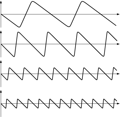
In the previous section, we saw that a lower bound on the MMSE can be obtained by solving the minimization problem (13). However, at this point, we have no guarantee that the solution $s$ of (13) is anywhere near the true value of the MMSE. Indeed, at first sight, it may appear that $s=0$ for any estimation setting. To see this, note that $Z[{\boldsymbol{b}}]$ is a sum of two components, a bias gradient part and a squared bias part. Both parts are nonnegative, but the former is zero when the bias gradient is $-{\boldsymbol{I}}$, while the latter is zero when the bias is zero. No differentiable function ${\boldsymbol{b}}$ satisfies these two constraints simultaneously for all ${\boldsymbol{\theta}}$, since if the squared bias is everywhere zero, then the bias gradient is also zero. However, it is possible to construct a sequence of functions ${\boldsymbol{b}}^{(i)}$ for which both the bias gradient and the squared bias norm tend to zero for almost every value of ${\boldsymbol{\theta}}$. An example of such a sequence in a one-dimensional setting is plotted in Fig. 1. Here, a sequence ${\boldsymbol{b}}^{(i)}$ of smooth, periodic functions is presented. The function period tends to zero, and the percentage of the cycle in which the derivative equals $-1$ increases as $i$ increases. Thus, the pointwise limit of the function sequence is zero almost everywhere, and the pointwise limit of the derivative is $-1$ almost everywhere.

In the specific case shown in Fig. 1, it can be shown that the value of $Z[{\boldsymbol{b}}^{(i)}]$ does not tend to zero; in fact, $Z[{\boldsymbol{b}}^{(i)}]$ tends to infinity in this situation. However, our example illustrates that care must be taken when applying concepts from finite-dimensional optimization problems to variational calculus.

The purpose of this section is to show that $s>0$, so that the bound is meaningful, for any problem setting satisfying the regularity conditions of Section II-B. (This question was not addressed by Young and Westerberg [5].) While doing so, we develop some abstract concepts which will also be used when analyzing the asymptotic properties of the OBB in Section V.

As often happens with variational problems, it turns out that the minimum of (13) is not necessarily achieved by any continuously differentiable function. In order to guarantee an achievable minimum, one must instead minimize (13) over a slightly modified space, which is defined below. As explained in Section II-B, all bias functions are continuously differentiable, so that the minimizing function ultimately obtained, if it is not differentiable, will not be the bias of any estimator. However, as we will see, the minimum value of our new optimization problem is identical to the infimum of (13). Furthermore, this approach allows us to demonstrate several important theoretical properties of the OBB.

Let ${L^{2}}$ be the space of $p_{\boldsymbol{\theta}}$-measurable functions ${\boldsymbol{b}}:\Theta\rightarrow{\mathbb{R}}^{n}$ such that

Define the associated inner product

and the corresponding norm $\|{\boldsymbol{b}}\|_{L^{2}}^{2}\triangleq\left\langle{\boldsymbol{b}},{\boldsymbol{b}}\right\rangle_{L^{2}}$. Any function ${\boldsymbol{b}}\in{L^{2}}$ has a derivative in the distributional sense, but this derivative might not be a function. For example, discontinuous functions have distributional derivatives which contain a Dirac delta. If, for every $i$, the distributional derivative $\partial b_{i}/\partial{\boldsymbol{\theta}}$ of ${\boldsymbol{b}}$ is a function in ${L^{2}}$, then ${\boldsymbol{b}}$ is said to be weakly differentiable [32], and its weak derivative is the matrix function $\partial{\boldsymbol{b}}/\partial{\boldsymbol{\theta}}$. Roughly speaking, a function is weakly differentiable if it is continuous and its derivative exists almost everywhere.

The space of all weakly differentiable functions in ${L^{2}}$ is called the first-order Sobolev space [32], and is denoted ${H^{1}}$. Define an inner product on ${H^{1}}$ as

The associated norm is $\|{\boldsymbol{b}}\|_{H^{1}}^{2}\triangleq\left\langle{\boldsymbol{b}},{\boldsymbol{b}}\right\rangle_{H^{1}}$. An important property which will be used extensively in our analysis is that ${H^{1}}$ is a Hilbert space.

Note that since $\Theta$ is an open set, not all functions in ${C^{1}}$ are in ${H^{1}}$. For example, in the case $\Theta={\mathbb{R}}^{n}$, the function ${\boldsymbol{b}}({\boldsymbol{\theta}})={\boldsymbol{k}}$, for some nonzero constant ${\boldsymbol{k}}$, is continuously differentiable but not integrable. Thus ${\boldsymbol{b}}$ is in ${C^{1}}$ but not in ${H^{1}}$, nor even in ${L^{2}}$. However, any measurable function which is not in ${H^{1}}$ has $\|{\boldsymbol{b}}\|_{H^{1}}=\infty$, meaning that either ${\boldsymbol{b}}$ or $\partial{\boldsymbol{b}}/\partial{\boldsymbol{\theta}}$ has infinite ${L^{2}}$ norm. Consequently, either the bias norm part or the bias gradient part of $Z[{\boldsymbol{b}}]$ is infinite. It follows that performing the minimization (13) over ${C^{1}}\cap{H^{1}}$, rather than over ${C^{1}}$, does not change the minimum value. On the other hand, ${C^{1}}\cap{H^{1}}$ is dense in ${H^{1}}$, and $Z[{\boldsymbol{b}}]$ is continuous, so that minimizing (13) over ${H^{1}}$ rather than ${C^{1}}\cap{H^{1}}$ also does not alter the minimum. Consequently, we will henceforth consider the problem

The advantage of including weakly differentiable functions in the minimization is that a unique minimizer can now be guaranteed, as demonstrated by the following result.

Proving the unique existence of a minimizer for (17) is a technical exercise in functional analysis which can be found in Appendix B. However, once the existence of such a minimizer is demonstrated, it is not difficult to see that $0<s<\infty$. To see that $s<\infty$, we must find a function ${\boldsymbol{b}}$ for which $Z[{\boldsymbol{b}}]<\infty$. One such function is ${\boldsymbol{b}}={\bf 0}$, for which $Z[{\boldsymbol{b}}]$ is finite since ${\boldsymbol{J}}({\boldsymbol{\theta}})$ is bounded. Now suppose by contradiction that $s=0$, which implies that there exists a function $\bar{{\boldsymbol{b}}}\in{H^{1}}$ such that $Z[\bar{{\boldsymbol{b}}}]=0$. Therefore, both the bias gradient and the squared bias parts of $Z[\bar{{\boldsymbol{b}}}]$ are zero. In particular, since the squared bias part equals zero, we have $\|\bar{{\boldsymbol{b}}}\|_{L^{2}}=0$. Hence, $\bar{{\boldsymbol{b}}}={\bf 0}$, because ${L^{2}}$ is a normed space. But then, by the definition (12) of $Z[\cdot]$,

which is positive; this is a contradiction.

Note that functions in ${H^{1}}$ are defined up to changes on a set having zero measure. In particular, the fact that ${\boldsymbol{b}}^{(0)}$ is unique does not preclude functions which are identical to ${\boldsymbol{b}}^{(0)}$ almost everywhere (which obviously have the same value $Z[{\boldsymbol{b}}]$).

Summarizing the discussion of the last two sections, we have the following theorem.

Two remarks are in order concerning Theorem 1. First, the function ${\boldsymbol{b}}$ solving (20) might not be the bias of any estimator; indeed, under our assumptions, all bias functions are continuously differentiable, whereas ${\boldsymbol{b}}$ need only be weakly differentiable. Nevertheless, (20) is still a lower bound on the MMSE. Another important observation is that Theorem 1 arises from the deterministic CRB; hence, there are no requirements on the prior distribution $p_{\boldsymbol{\theta}}({\boldsymbol{\theta}})$. In particular, $p_{\boldsymbol{\theta}}({\boldsymbol{\theta}})$ can be discontinuous or have bounded support. By contrast, many previous Bayesian bounds do not apply in such circumstances.

In finite-dimensional convex optimization problems, the requirement of a vanishing first derivative results in a set of equations, whose solution is the global minimum. Analogously, in the case of convex functional optimization problems such as (20), the optimum is given by the solution of a set of differential equations. The following theorem, whose proof can be found in Appendix C, specifies the differential equation relevant to our optimization problem.

In this section and in the remainder of the paper, we will consider the case in which the set $\Theta=\{{\boldsymbol{\theta}}:p_{\boldsymbol{\theta}}({\boldsymbol{\theta}})>0\}$ is bounded. From a practical point of view, even when $\Theta$ consists of the entire set ${\mathbb{R}}^{n}$, it can be approximated by a bounded set containing only those values of ${\boldsymbol{\theta}}$ for which $p_{\boldsymbol{\theta}}({\boldsymbol{\theta}})>\epsilon$.

Note that Theorem 1 guarantees the existence of a unique solution in ${H^{1}}$ to the differential equation (21) with the boundary conditions (22).

The bound of Young and Westerberg [5] is a special case of Theorem 2, and is given here for completeness.

Theorem 2 can be solved numerically, thus obtaining a bound for any problem satisfying the regularity conditions. However, directly solving (21) becomes increasingly complex as the dimension of the problem increases. Instead, in many cases, symmetry relations in the problem can be used to simplify the solution. As an example, the following spherically symmetric case can be reduced to a one-dimensional setting equivalent to that of Corollary 1. The proof of this theorem can be found in Appendix D.

In this theorem, the requirement ${\boldsymbol{J}}({\boldsymbol{\theta}})=J(\|{\boldsymbol{\theta}}\|){\boldsymbol{I}}$ indicates that the Fisher information matrix is diagonal and that its components are spherically symmetric. Parameters having a diagonal matrix ${\boldsymbol{J}}$ are sometimes referred to as orthogonal. The simplest case of orthogonality occurs when, to each parameter $\theta_{i}$, there corresponds a measurement $x_{i}$, in such a way that the random variables $x_{i}|{\boldsymbol{\theta}}$ are independent. Other orthogonal scenarios can often be constructed by an appropriate parametrization [33].

The requirement that ${\boldsymbol{J}}$ have spherically symmetric components occurs, for example, in location problems, i.e., situations in which the measurements have the form ${\boldsymbol{x}}={\boldsymbol{\theta}}+{\boldsymbol{w}}$, where ${\boldsymbol{w}}$ is additive noise which is independent of ${\boldsymbol{\theta}}$. Indeed, under such conditions, ${\boldsymbol{J}}$ is constant in ${\boldsymbol{\theta}}$ [31, §3.1.3]. If, in addition, the noise components are independent, then this setting also satisfies the orthogonality requirement, and thus application of Theorem 3 is appropriate. Note that this estimation problem is not separable, since the components of ${\boldsymbol{\theta}}$ are correlated; thus, the MMSE in this situation is lower than the sum of the components’ MMSE. An example of such a setting is presented in Section VI.

In this section, we examine several properties of the OBB. We first demonstrate that the optimal bias function has zero mean, a property which also characterizes the bias function of the MMSE estimator. Next, we prove that, under very general conditions, the resulting bound is tight at both low and high SNR values. This is an important result, since a desirable property of a Bayesian bound is that it provides an accurate estimate of the ambiguity region between high and low SNR [11]. Reliable estimation at the two extremes increases the likelihood that the transition between these two regimes will be correctly identified.

The original bound of Young and Westerberg [5] predates most Bayesian bounds, and, surprisingly, it has never been cited by or compared with later results. In this section, we measure the performance of the original bound and of its extension to the vector case against that of various other techniques. We consider the case in which ${\boldsymbol{\theta}}$ is uniformly distributed over an $n$-dimensional open ball $\Theta=\{{\boldsymbol{\theta}}:\|{\boldsymbol{\theta}}\|<r\}\subseteq{\mathbb{R}}^{n}$, so that

where $\mathbbm{1}_{S}$ equals $1$ when ${\boldsymbol{\theta}}\in S$ and $0$ otherwise, and

is the volume of an $n$-ball of radius $r$ [35]. We further assume that

where ${\boldsymbol{w}}$ is zero-mean Gaussian noise, independent of ${\boldsymbol{\theta}}$, having covariance $\sigma^{2}{\boldsymbol{I}}$. We are interested in lower bounds on the MSE achievable by an estimator of ${\boldsymbol{\theta}}$ from ${\boldsymbol{x}}$.

We begin by developing the OBB for this setting, as well as some alternative bounds. We then compare the different approaches in a one-dimensional and a three-dimensional setting.

The Fisher information matrix for the given estimation problem is given by ${\boldsymbol{J}}({\boldsymbol{\theta}})=\sigma^{-2}{\boldsymbol{I}}$, so that the conditions of Theorem 3 hold. It follows that the optimal bias function is given by ${\boldsymbol{b}}({\boldsymbol{\theta}})=b(\|{\boldsymbol{\theta}}\|){\boldsymbol{\theta}}/\|{\boldsymbol{\theta}}\|$, where $b(\cdot)$ is a solution to the differential equation

with boundary conditions $b(0)=0$, $b^{\prime}(r)=-1$. The general solution to this differential equation is given by

where $I_{\alpha}\!\left({z}\right)$ and $K_{\alpha}\!\left({z}\right)$ are the modified Bessel functions of the first and second types, respectively [36]. Since $K_{\alpha}\!\left({z}\right)$ is singular at the origin, the requirement $b(0)=0$ leads to $C_{2}=0$. Differentiating (39) with respect to $\theta$, we obtain

so that the requirement $b^{\prime}(r)=-1$ leads to

Substituting this value of $b(\cdot)$ into (24) yields the OBB, which can be computed by evaluating a single one-dimensional integral. Alternatively, in the one-dimensional case, the integral can be computed analytically, as will be shown below.

Despite the widespread use of finite-support prior distributions [10, 4], the regularity conditions of many bounds are violated by such prior pdf functions. Indeed, the Bayesian CRB of Van Trees [3], the Bobrovski–Zakai bound [8], and the Bayesian Abel bound [12] all assume that $p_{\boldsymbol{\theta}}({\boldsymbol{\theta}})$ has infinite support, and thus cannot be applied in this scenario.

Techniques from the Ziv–Zakai family are applicable to constrained problems. An extension of the Ziv–Zakai bound for vector parameter estimation was developed by Bell et al. [11]. From [11, Property 4], the MSE of the $i$th component of ${\boldsymbol{\theta}}$ is bounded by

where ${\boldsymbol{e}}_{i}$ is a unit vector in the direction of the $i$th component, $V\{\cdot\}$ is the valley-filling function defined by

and $P_{\min}({\boldsymbol{\delta}})$ is the minimum probability of error for the problem of testing hypothesis $H_{0}:{\boldsymbol{\theta}}={\boldsymbol{\theta}}_{0}$ vs. $H_{1}:{\boldsymbol{\theta}}={\boldsymbol{\theta}}_{0}+{\boldsymbol{\delta}}$. In the current setting, $P_{\min}({\boldsymbol{\delta}})$ is given by $P_{\min}({\boldsymbol{\delta}})=Q\!\left(\|{\boldsymbol{\delta}}\|/2\sigma\right)$, where $Q\!\left(z\right)=(2\pi)^{-1/2}\int_{z}^{\infty}e^{-t^{2}/2}dt$ is the tail function of the normal distribution. Also, we have

where

and $\Theta+h{\boldsymbol{e}}_{1}=\{{\boldsymbol{\theta}}+h{\boldsymbol{e}}_{1}:{\boldsymbol{\theta}}\in\Theta\}$. Thus, $V_{n}^{C}(r,h)$ is the volume of the intersection of two $n$-balls whose centers are at a distance of $h$ units from one another. Substituting these results into (42), we have

Note that both $V_{n}^{C}(r,\|{\boldsymbol{\delta}}\|)$ and $Q(\|{\boldsymbol{\delta}}\|/2\sigma)$ decrease with $\|{\boldsymbol{\delta}}\|$. Therefore, the maximum in (47) is obtained for ${\boldsymbol{\delta}}=h{\boldsymbol{e}}_{i}$. Also, since the argument of $V\{\cdot\}$ is monotonically decreasing, the valley-filling function has no effect and can be removed. Finally, since $V_{n}^{C}(r,h)=0$ for $h>2r$, the integration can be limited to the range $[0,2r]$. Thus, the extended Ziv–Zakai bound is given by

We now compute the Weiss–Weinstein bound for the setting at hand. This bound is given by

where ${\boldsymbol{H}}=[{\boldsymbol{h}}_{1},\ldots,{\boldsymbol{h}}_{m}]$ is a matrix containing an arbitrary number $m$ of test vectors and ${\boldsymbol{G}}$ is a matrix whose elements are given by

in which

and

The vectors ${\boldsymbol{h}}_{1},\ldots,{\boldsymbol{h}}_{m}$ and the scalars $s_{1},\ldots,s_{m}$ are arbitrary, and can be optimized to maximize the bound (49). To avoid a multidimensional nonconvex optimization problem, we restrict attention to $m=n$, ${\boldsymbol{h}}_{i}=h{\boldsymbol{e}}_{i}$, and $s_{i}=1/2$, as suggested by [10]. This results in a dependency on a single scalar parameter $h$.

Under these conditions, $G_{ij}$ can be written as

References

• [1] J. O. Berger, Statistical Decision Theory and Bayesian Analysis, 2nd ed. New York, NY: Springer-Verlag, 1985.
• [2] S. M. Kay, Fundamentals of Statistical Signal Processing: Estimation Theory. Englewood Cliffs, NJ: Prentice Hall, 1993.
• [3] H. L. Van Trees, Detection, Estimation, and Modulation Theory. New York: Wiley, 1968, vol. 1.
• [4] J. Ziv and M. Zakai, “Some lower bounds on signal parameter estimation,” IEEE Trans. Inf. Theory, vol. 15, no. 3, pp. 386–391, May 1969.
• [5] T. Y. Young and R. A. Westerberg, “Error bounds for stochastic estimation of signal parameters,” IEEE Trans. Inf. Theory, vol. 17, no. 5, pp. 549–557, Sep. 1971.
• [6] S. Bellini and G. Tartara, “Bounds on error in signal parameter estimation,” IEEE Trans. Commun., vol. 22, no. 3, pp. 340–342, 1974.
• [7] D. Chazan, M. Zakai, and J. Ziv, “Improved lower bounds on signal parameter estimation,” IEEE Trans. Inf. Theory, vol. 21, no. 1, pp. 90–93, 1975.
• [8] B. Z. Bobrovski and M. Zakai, “A lower bound on the estimation error for certain diffusion problems,” IEEE Trans. Inf. Theory, vol. 22, no. 1, pp. 45–52, Jan. 1976.
• [9] A. J. Weiss and E. Weinstein, “A lower bound on the mean-square error in random parameter estimation,” IEEE Trans. Inf. Theory, vol. 31, no. 5, pp. 680–682, Sep. 1985.
• [10] E. Weinstein and A. J. Weiss, “A general class of lower bounds in parameter estimation,” IEEE Trans. Inf. Theory, vol. 34, no. 2, pp. 338–342, Mar. 1988.
• [11] K. L. Bell, Y. Steinberg, Y. Ephraim, and H. L. Van Trees, “Extended Ziv–Zakai lower bound for vector parameter estimation,” IEEE Trans. Inf. Theory, vol. 43, no. 2, pp. 624–637, 1997.
• [12] A. Renaux, P. Forster, P. Larzabal, and C. Richmond, “The Bayesian Abel bound on the mean square error,” in Proc. Int. Conf. Acoust., Speech and Signal Processing (ICASSP 2006), vol. III, Toulouse, France, May 2006, pp. 9–12.
• [13] E. L. Lehmann and G. Casella, Theory of Point Estimation, 2nd ed. New York: Springer, 1998.
• [14] Y. C. Eldar, “Rethinking biased estimation: Improving maximum likelihood and the Cramér–Rao bound,” Foundations and Trends in Signal Processing, vol. 1, no. 4, pp. 305–449, 2008.
• [15] S. M. Kay and Y. C. Eldar, “Rethinking biased estimation,” IEEE Signal Process. Mag., vol. 25, no. 3, pp. 133–136, May 2008.
• [16] H. Cramér, “A contribution to the theory of statistical estimation,” Skand. Akt. Tidskr., vol. 29, pp. 85–94, 1945.
• [17] C. R. Rao, “Information and accuracy attainable in the estimation of statistical parameters,” Bull. Calcutta Math. Soc., vol. 37, pp. 81–91, 1945.
• [18] J. M. Hammersley, “On estimating restricted parameters,” J. Roy. Statist. Soc. B, vol. 12, no. 2, pp. 192–240, 1950.
• [19] D. G. Chapman and H. Robbins, “Minimum variance estimation without regularity assumptions,” Ann. Math. Statist., vol. 22, no. 4, pp. 581–586, Dec. 1951.
• [20] P. K. Bhattacharya, “Estimating the mean of a multivariate normal population with general quadratic loss function,” Ann. Math. Statist., vol. 37, no. 6, pp. 1819–1824, Dec. 1966.
• [21] E. W. Barankin, “Locally best unbiased estimates,” Ann. Math. Statist., vol. 20, no. 4, pp. 477–501, Dec. 1949.
• [22] J. S. Abel, “A bound on mean-square-estimate error,” IEEE Trans. Inf. Theory, vol. 39, no. 5, pp. 1675–1680, 1993.
• [23] A. O. Hero, J. A. Fessler, and M. Usman, “Exploring estimator bias-variance tradeoffs using the uniform CR bound,” IEEE Trans. Signal Process., vol. 44, no. 8, pp. 2026–2041, 1996.
• [24] P. Forster and P. Larzabal, “On lower bounds for deterministic parameter estimation,” in Proc. Int. Conf. Acoust., Speech and Signal Processing (ICASSP 2002), vol. 2, Orlando, FL, May 2002, pp. 1137–1140.
• [25] Y. C. Eldar, “Minimum variance in biased estimation: Bounds and asymptotically optimal estimators,” IEEE Trans. Signal Process., vol. 52, no. 7, pp. 1915–1930, 2004.
• [26] ——, “Uniformly improving the Cramér-Rao bound and maximum-likelihood estimation,” IEEE Trans. Signal Process., vol. 54, no. 8, pp. 2943–2956, 2006.
• [27] ——, “MSE bounds with affine bias dominating the Cramér–Rao bound,” IEEE Trans. Signal Process., vol. 56, no. 8, pp. 3824–3836, Aug. 2008.
• [28] I. A. Ibragimov and R. Z. Has’minskii, Statistical Estimation: Asymptotic Theory. New York: Springer, 1981.
• [29] A. Renaux, “Contribution à l’analyse des performances d’estimation en traitement statistique du signal,” Ph.D. dissertation, Ècole Normale Superieure de Cachan, 2006. [Online]. Available: http://tel.archives-ouvertes.fr/tel-00129527/
• [30] Z. Ben-Haim and Y. C. Eldar, “A Bayesian estimation bound based on the optimal bias function,” in Proc. 2nd Int. Workshop on Computational Adv. in Multi-Sensor Adapt. Process. (CAMSAP 2007), St. Thomas, U.S. Virgin Islands, Dec. 2007.
• [31] J. Shao, Mathematical Statistics, 2nd ed. New York: Springer, 2003.
• [32] E. H. Lieb and M. Loss, Analysis, 2nd ed. American Mathematical Society, 2001.
• [33] D. R. Cox and N. Reid, “Parameter orthogonality and approximate conditional inference,” J. Roy. Statist. Soc. B, vol. 49, no. 1, pp. 1–39, 1987.
• [34] H. L. Van Trees and K. L. Bell, Bayesian Bounds for Parameter Estimation and Nonlinear Filtering/Tracking. New York: Wiley, 2007.
• [35] I. M. Vinogradov, Ed., Encyclopaedia of Mathematics. Dordrecht, The Netherlands: Kluwer, 1995.
• [36] M. Abramowitz and I. A. Stegun, Handbook of Mathematical Functions with Formulas, Graphs, and Mathematical Tables. New York: Dover, 1964.
• [37] Z. Ben-Haim and Y. C. Eldar, “A comment on the use of the Weiss–Weinstein bound with constrained parameter sets,” IEEE Trans. Inf. Theory, vol. 54, no. 10, pp. 4682–4684, Oct. 2008.
• [38] L. P. Lebedev and M. J. Cloud, The Calculus of Variations and Functional Analysis. New Jersey: World Scientific, 2003.
• [39] W. Rudin, Functional Analysis. New York: McGraw-Hill, 1973.
• [40] I. M. Gelfand and S. V. Fomin, Calculus of Variations. Mineola, NY: Dover, 2000.