Challenges for asteroseismic analysis of Sun-like stars
Abstract
Context. Asteroseismology of Sun-like stars is undergoing rapid expansion with, for example, new data from the CoRoT mission and continuation of ground-based campaigns. There is also the exciting upcoming prospect of NASA’s Kepler mission, which will allow the asteroseismic study of several hundred Sun-like targets, in some cases for periods lasting up to a few years.
Aims. The seismic mode parameters are the input data needed for making inference on stars and their internal structures. In this paper we discuss the ease with which it will be possible to extract estimates of individual mode parameters, dependent on the mass, age, and visual brightness of the star. Our results are generally applicable; however, we look at mode detectability in the context of the upcoming Kepler observations.
Methods. To inform our discussions we make predictions of various seismic parameters. To do this we use simple empirical scaling relations and detailed pulsation computations of the stochastic excitation and damping characteristics of the Sun-like p modes.
Results. The issues related to parameter extraction on individual p modes discussed here are mode detectability, the detectability and impact of stellar activity cycles, and the ability to measure properties of rotationally split components, which is dependent on the relative importance of the rotational characteristics of the star and the damping of the stochastically excited p modes.
Key Words.
stars: oscillations – stars: activity – Sun: activity – Sun: helioseismology – data analysis1 Introduction
With the recent launch of CoRoT (Baglin et al. 2006), the upcoming launch of NASA’s Kepler mission (Basri et al. 2005) and continuation of observations by MOST (Matthews et al. 2007) and ground-based teams (Bedding & Kjeldsen 2006), we are entering a rewarding era for asteroseismic studies of the interiors of Sun-like stars. Sun-like oscillations give a very rich spectrum allowing internal structures and dynamics to be probed down into the stellar cores to very high precision. Asteroseismic observations of many stars will allow multiple-point tests of crucial aspects of stellar evolution and dynamo theory.
The prospects for asteroseismology with Kepler are particularly exciting. In addition to searching for Earth-like exoplanets (via the transit method), the Kepler Asteroseismology Investigation (KAI) – which is arranged around the Kepler Asteroseismic Science Operations Centre (KASOC) – will provide an unprecedented opportunity to study several hundred stars showing Sun-like oscillations (Christensen-Dalsgaard et al. 2007, 2008). Because the nominal mission lifetime is 3.5 years we should expect to have long datasets on many of these stars.
The input data for probing stellar interiors are the mode parameters, such as individual frequencies, frequency splittings, linewidths, and powers. For those stars where measurement of individual mode parameters is difficult, the input data will be ensemble averages, e.g., mean frequency spacings. Accurate mode parameter data are a vital prerequisite for robust, accurate inference on the internal structures of the stars. Asteroseismic observations covering periods of several years will also allow studies of stellar cycles from observation of systematic stellar-cycle-driven variations of the mode parameters, thereby giving important information to the dynamo theorists.
Parameters of individual modes may be estimated using the “peak-bagging” fitting techniques, which have been applied to Sun-as-a-star helioseismology data (e.g., Chaplin et al. 2006) and which are now being applied to Sun-like asteroseismology data, e.g., the CoRoT data (Appourchaux et al. 2006a, b) and also WIRE spacecraft data (Fletcher et al. 2006; Karoff et al. 2007). Peak-bagging involves maximum-likelihood fitting of mode peaks in the frequency power spectrum to multi-parameter fitting models, where individual mode peaks are represented by Lorentzian-like functions. The parameters may also be extracted using methods which have been developed for analysis of ground-based data on Sun-like stars (e.g., see Bedding et al. 2004; Kjeldsen et al. 2005). For example, from measurement of the variance, over time, of frequency locations of peaks it is possible to estimate the intrinsic damping rates of stochastically excited modes.
In this paper we are concerned with making predictions of the ease with which it will be possible to extract estimates of parameters on individual low-degree (low-) acoustic (p) modes, in different regions of the HR diagram occupied by the Sun-like oscillators. We do so with an eye on the upcoming Kepler observations. To make our predictions we use simple empirical scaling relations, together with detailed pulsation computations of the stochastic excitation and damping characteristics of the p modes. The predictions and discussions that follow are by no means exhaustive. However, they do cover several important issues that are relevant to the challenge of extracting estimates of parameters on individual modes. The main issues we consider, for stars of different mass and age, are:
- •
The detectability of modes;
- •
The impact of stellar activity cycles on the observed mode peaks. We comment on detectability of those cycles; we also consider changes to the mode power and damping rates, which have implications not only for detectability but also detailed comparison of observations with theoretical predictions of the excitation and damping; and
- •
The ability to resolve individual components in the non-radial mode multiplets, which depends on the relative importance of rotation and mode damping.
The layout of our paper is as follows. We begin in Section 2 with a brief description of the pulsation calculations, which are performed for a grid of 31 stellar models. We then look in Section 3 at predictions of the mode powers and widths for the models and discuss detectability issues in the context of noise levels expected for the Kepler observations, which will be photometric. In Section 4, we use empirical scaling relations to predict stellar-cycle characteristics for our grid of stellar models and use these predictions to comment on the variability we might expect in estimates of p-mode frequencies, powers and damping rates. Our discussion on stellar-cycle variability also includes a look at how shapes of mode peaks in the frequency power spectrum may be distorted by strong cycles. Finally, in Section 5 we use empirical predictions of surface rotation rates to comment on the difficulty of resolving components in non-radial mode multiplets. We then draw together the main summary points in Section 6.
2 Stellar model data
We have considered a grid of stellar models, with masses in the range 0.7 to and ages in the range from the ZAMS to 9 Gyr. We used the Padova isochrones (Bonatto, Bica & Girardi 2004; Girardi et al. 2002, 2004) to specify the primary characteristics of each model, i.e., mass , radius , effective temperature , and luminosity . The composition was fixed at and for all models. Fig. 1 shows a luminosity-effective temperature plot (left-hand panel) and an age-effective temperature plot (right-hand panel), for the models. The different symbols denote models of different mass (see caption).
The stellar equilibrium and pulsation computations that we performed are as described by Balmforth (1992), Houdek et. al (1999), and Chaplin et al. (2005). The pulsation computations required estimates of , , and the composition as input. The computations gave as output estimates of the acoustic powers and damping rates of the radial p modes of each stellar model. We essentially followed the same recipe to perform the computations as Chaplin et al. (2007). However, whereas in Chaplin et al. we performed computations for 22 stellar models whose input parameters were chosen to match those of stars that have been observed by the Mount Wilson Ca II H&K program, here we instead performed computations for the grid of 31 models having basic parameters to reflect systematic variations in mass and age.


3 Mode heights and widths in the frequency power spectrum
Information on the p modes may be extracted by, for example, analysis of the p-mode peaks in the frequency power spectrum. Here, we use the results of the stellar model computations to make predictions of the peak parameters. The stellar model computations provided predictions of two independent sets of radial-mode parameters for each star: the linear damping rates, , and the excitation rates (acoustic powers), . The observed parameters of the mode peaks in the frequency power spectrum are formed from these quantities. The peak fwhm linewidths are given by while the velocity powers, , are calculated from (e.g., Houdek et al. 1999):
| (1) |
Here, is the mode inertia. The computations were calibrated so that for a model of the Sun the maximum rms mode amplitude was .
In order to predict mode amplitudes, , in intensity – to allow us to discuss results in the context of the photometric Kepler observations – we convert from the velocity amplitudes, , using (Kjeldsen & Bedding 1995):
| (2) |
The spectral fwhm bandpass of Kepler runs from 430 to 890 nm. We therefore used an average wavelength of in Equation 2 above.
If observations are of sufficient length to resolve mode peaks in the frequency power spectrum the (or ) do not give the observed heights of the peaks. The requirement for peaks to be resolved may be put in terms of the mode lifetime . The requirement is that the observation length (Chaplin et al. 2003). When the peaks are resolved, the heights – or maximum power spectral densities – are instead given by (Chaplin et al. 2005):
| (3) |
In what follows as shall assume the condition is met for the observations. We make some comments on this assumption in Appendix A. Furthermore, we use rms amplitudes, , to calculate the heights .
3.1 Frequency at maximum mode height

It has been shown that for the Sun-like oscillators, the frequency of maximum power of the p modes scales to good approximation with the acoustic cut-off frequency (Bedding & Kjeldsen 2003). The frequency of maximum power for the radial solar p modes is . We use this value to calibrate the following scaling relation:
| (4) |
How well do the pulsation computations match this relation? We consider the match for computations of the heights, , as opposed to the amplitudes, , since it is the heights that determine the detectability of modes in the frequency power spectrum.
In Fig. 2 we plot the frequency of maximum height from the model computations against the scaled frequency from Equation 4. The dotted line shows the locus along which the pulsation computation results would lie should they follow Equation 4. While the match is reasonable for most of the models, there are results for two sequences of models which lie a long way from the dotted line. These are results on the lighter and models, where the pulsation computations actually show two maxima in (see Fig. 3). We plot data in Fig. 2 for the two maxima at each mass: at both masses one maximum lies close to the line, while the other does not.
The presence of a second maximum is due predominantly to local depressions in the linear damping rates (as a function of frequency), as was pointed out by Chaplin et al. (2007). For the models, at the higher-frequency maximum is always larger than at the lower-frequency maximum (see left-hand panel of Fig. 3). The frequency locations of these higher-frequency maxima are plotted as full-sized asterisks in Fig. 2 and are seen to lie closer to the curve than their out-of-line, lower-frequency counterparts (the latter plotted as small asterisks). For the models it is the lower-frequency maxima that are the more prominent (see right-hand panel of Fig. 3), and which also follow more closely the linear scaling with (see full-sized diamonds in Fig. 2). In what follows we use pulsation computation results on modes at the strongest maxima.


3.2 Height-to-background ratios in Kepler data
In order to give some observational context for the computed heights, , here we compare them with shot noise power spectral densities predicted for intensity observations by the Kepler instrument.
First, we follow the procedure in Chaplin et al. (2007) and average calculated heights from the pulsation computations over the five strongest radial modes, to give . Fig. 4 shows the resulting estimates of , in units of . The dashed line shows the average for the five strongest solar radial modes. By averaging results we get predictions for the detectability of several overtones. Also plotted (dotted lines) are the noise power spectral density levels, , expected for Kepler observations at (lowest-lying line) to 15 (top line). These levels were calculated from:
| (5) |
where is the cadence (60 sec) and are the estimated Kepler shot noise levels, per 60-sec sample (Kjeldsen, private communication). The selected span the nominal apparent magnitude target range for Kepler.
We have plotted and against not only effective temperature (left-hand panel of Fig. 4), but also half the average large frequency spacing (right-hand panel). This is the dominant frequency spacing of the low- frequency power spectrum, it being approximately the spacing between consecutive odd- ( and 3) and even- ( and 2) mode pairs.
Fig. 5 shows similar plots, this time for the average linewidths, , from the pulsation computations. These averages were again made over the five strongest modes in each model.


Let us consider some of the important points to take from Figs. 4 and 5:
- •
While the average heights, , increase by approximately two orders of magnitude going from the to the models, the average linewidths , in contrast increase by only approximately a factor of three to four. For a given evolutionary sequence average heights increase with increasing age. The behaviour of the average linewidths, , is more complicated. Up to mass , each evolutionary sequence shows an overall increase in average linewidth with increasing age. The changes can be far from monotonic and are typically quite modest, e.g., for the sequence the change in from the ZAMS to 9 Gyr amounts to only about 20 %. At higher mass things get more complicated. The average linewidths of the sequence first increase, then decrease. At there is a pronounced decrease in average linewidth with increasing age.
- •
The best potential targets for extracting estimates of individual mode parameters are of course the more massive models, for which we expect to have good height-to-background ratios in the frequency power spectrum. However, this comes at a cost. First, the tendency is for the damping to be stronger in these more massive models, compared to their lighter counterparts. Since mode peaks are therefore wider in the frequency power spectrum, the data will be more susceptible to blending effects between adjacent mode components, making clean extraction of frequency spacings or splittings harder. The problem of blending can cause severe problems for attempts to estimate the angle of inclination offered by the star. The inclination affects the relative amplitudes of rotationally split components in non-radial modes, meaning it can in principle be constrained if the amplitude ratios can be measured. This will not be possible in the presence of significant blending. Convergence to, or use of, poor estimates of the inclination can also significantly bias estimates of the frequency splittings. Even a factor-of-two difference in the widths can have a big impact on the analysis (e.g., see Gizon & Solanki 2003; Ballot et al. 2006, 2008).
While the magnitudes of the linewidths do give some guide to potential problems, a much more useful measure is the ratio of the rotational frequency splittings to the linewidths. This ratio determines how easy it is to resolve adjacent components in the non-radial modes. We go on to discuss issues concerning rotation, including predictions of the splitting-to-linewidth ratio, later in Section 5.
The second problem for the more massive models is that they show the smallest large frequency spacings. This means power from adjacent outlying overtones can have a significant contribution in the frequency neighbourhood of a mode whose properties are being estimated. A common peak-bagging approach is to go through the frequency power spectrum fitting a mode pair at a time. This is because the modes lie in close proximity in frequency to the modes. The same is true for the and modes. Since the fitting models usually only include power from the target pair, power in the target frequency window from other outlying modes – which is not accounted for in the fitting models – can bias the best-fitting parameters (e.g., see discussion in Fletcher et al. 2008). A way round this is of course to take account of the outlying power (e.g., Gelly et al. 2002; Jimenéz, Roca-Cortés & Jimenéz-Reyes 2002; Fletcher et al. 2008), or to fit all modes in the frequency power spectrum in one go (e.g., see Lazrek et al., 2001; Appourchaux 2003; Jefferies, Vorontsov & Giebink 2004). Techniques like these may need to be called into play when long Kepler datasets are analyzed on the more massive Sun-like oscillators.
- •
From ground-based observations of the p-mode spectrum of Procyon is has been established that analytical predictions of the mode amplitudes overestimate the observed amplitudes in this hottest part of the ‘Sun-like’ regime, e.g., see the discussion in Houdek (2006) and references therein. The discrepancy is approximately a factor of five in power for Procyon, which has an effective temperature of (Allende Prieto et al. 2002). Even if one were to reduce the heights of the models (diagonal crosses) in this paper by a factor of five the expected height-to-background ratios would remain healthy for observations at the bright end of the target range of Kepler. Some of the discrepancy between the pulsation computations and the observations is most likely due to an underestimation of the damping rates by the computations. As such, the mode widths may if anything be larger in this part of the HR diagram than the predictions shown in Fig. 5, which may add to complications for parameter estimation of individual modes.
- •
The height and noise data in Fig. 4 suggest it may not be possible to extract parameters on individual modes from some of the lightest stars in the Kepler field.
4 Stellar cycle effects
Next, we consider the impact of stellar cycle effects on the p-mode parameters of Sun-like oscillators. From our experience of analyzing helioseismic data we expect not only the mode frequencies, but also the mode heights and linewidths, to show stellar-cycle variations. We begin by using scaling relations to predict the sizes of the stellar-cycle changes for each member of our grid of stellar models.
4.1 Predicted stellar-cycle shifts
A commonly used indicator of surface activity on stars is the Ca II H&K index. This index is usually expressed as , the average fraction of the star’s total luminosity that is emitted in the H&K line cores (having been corrected for the photospheric component). In order to give first-order estimates of the stellar-cycle shifts in the p modes, we have made use of data on 22 main-sequence stars that have been observed by the Mount Wilson Ca II H&K program (Radick et al. 1998; Saar & Brandenburg 2002; see also Baliunas et al. 1995) to have well-defined, and measurable, stellar activity cycles in . These data, which come from Saar & Brandenburg, are the same data that were used in Chaplin et al. (2007) and we refer the reader to that paper for more details. Here, we give a brief summary of how we estimated mean p-mode frequency shifts from these data.
First, we turned the data (the cycle amplitudes in ) into first-order estimates of mean p-mode frequency shifts by simply scaling against the 0.4- frequency shift seen for the most prominent low- modes on the Sun. In doing so, we assumed that the low- shifts scale approximately linearly with . A linear fit of the estimated p-mode frequency shifts versus the observed then served as a look-up curve to calculate a mean p-mode frequency shift for the most prominent modes of each of the 31 models in this paper. There is some uncertainty in our simple scaling due to the unknown inclination, , of the stars. We attempted to make some allowance for this by weighting the fits, using the estimated uncertainties discussed in Chaplin et al. (2007) as weights.
In order to use the resulting look-up curve we first had to estimate the of each model. We used scaling relations due to Noyes (1983) and Noyes et al. (1984), which require and the surface rate of rotation, to estimate the of our model stars. We discuss how we estimated the rotation rates in Section 5 below. Estimated stellar-cycle frequency shifts for the most prominent modes of the 31 models are plotted in the top left-hand panel of Fig. 6. Because these predictions rely on predictions of the surface rates of rotation, which are more uncertain for the ZAMS models, the youngest data we show here are the 1-Gyr results (bold symbols). For each mass, one should pan down the symbols to go to older models. We therefore see that the predicted amplitudes of the stellar cycles decrease monotonically with age for all but the two most massive model sequences.
The right-hand axis of the top left-hand panel of Fig. 6 shows the scale for the predicted fractional changes in the average heights, , of the stellar models (those in the average linewidths, , are half the size). As with the frequency shifts, we have scaled the shifts of the heights and widths using the known solar values. The absolute fractional change, from activity minimum to maximum, in the of the low- solar p modes is about 40 %. That in is about 20 % (Chaplin et al. 2000).
Chaplin et al. (2007) discussed at length the prospects for detecting signatures of stellar activity cycles in the p-mode frequency shifts. They concluded that provided modes covering several radial orders are observed at reasonable S/N, it should be possible to measure the parameter shifts given only a few multi-month segments of data. The results here reinforce these conclusions: the top left-hand panel of Fig. 6 shows that most of the predicted stellar-cycle frequency shifts have larger amplitudes than the Sun.
Prospects for detecting the stellar-cycle shifts from observations of finite length depend not only on the amplitudes of the cycles, but also on the cycle periods, . Take the case where the observations span less than half the cycle period. Then for a given cycle amplitude, the shorter the cycle period, the larger will be the observed frequency shift. In order to take account of this dependence, the top right-hand panel of Fig. 6 plots the predicted cycle shifts multiplied by the ratio . (Appendix B explains how we derived estimates of .) The majority of these normalized shifts are again seen to be larger than for the Sun.


The bottom panels of Fig. 6 plot the average heights and average linewidths, and respectively (Fig. 4). However, this time we also use error bars to show estimated lower and upper bounds on the parameters, from our predictions of the stellar cycles. The of the younger models – which in some cases have estimated cycle shifts that are between one-and-a-half and two-times stronger than the Sun – are predicted to vary by as much as %. When we make detailed comparisons of predictions of – from the analytical pulsation calculations, or from numerical simulations – with observations of , we therefore need to be sure we know whether stars show significant variations in activity, and if they do, at what point in any cycles the observations have been made. If information on the stellar cycles is not known a priori, our predictions imply that we cannot ensure the accuracy of any comparisons to better than (on average) about 50 % in .
Finally in this section, we note that the predicted widths in the bottom left-hand panel of Fig. 6 show an approximate linear dependence on the effective temperature, , in the range from to . The dotted line shows the best-fitting straight line for all models in this range. We used the error bars from the stellar-cycle predictions as weights for the straight-line fit, which is described by:
| (6) |
Equation 6 may be used to make predictions of the linewidths of the most prominent p modes of models having .
4.2 Distortion of mode peaks by stellar cycles
Large stellar-cycle frequency shifts can create potential problems for peak-bagging. The problems arise when the frequency power spectrum to be analyzed is made from a timeseries within which significant variation of the frequencies is present. The resonant peaks in the frequency power spectrum may then be distorted because of the frequency variations. The distortion means the peaks no longer have the Lorentzian-like shapes, on which the peak-bagging fitting models are based. These issues are discussed at length in Chaplin et al. (2008), where results on the expected distortions are presented for the solar case. While the distortions have little impact on estimates of the mode frequencies, they can bias estimation of the heights and widths, because the Lorentzian fitting models are no longer a good representation of the underlying peaks.
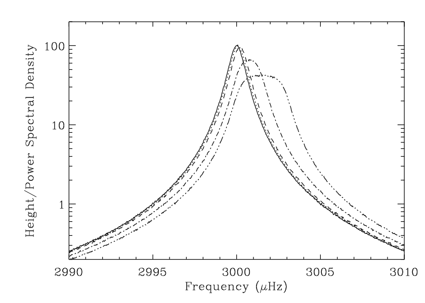
It turns out that the key parameter for determining the extent of any distortion is the ratio of the frequency shift, , in the timeseries to the peak linewidth. We call this ratio . Some examples of distorted peaks are shown in the top panel of Fig. 7, for values of , 0.15, 0.40, 1.50 and 3.00. Note that for the most prominent low- solar p modes (for which and ).
Aside from the change to the shape of the profiles, there are also clearly implications for mode detectability. The profiles characterized by and 3 have maximum heights that are, respectively, only % and 40 % of the height of the undistorted profile.
The bottom left-hand panel of Fig. 7 plots the estimated of our model stars. The dashed line shows the solar value. We see that the prediction implies cooler stars are more likely to show larger peak distortions. That said, we need to think a little harder about the prediction. When we compare one star with another, the estimated , which are used to compute , do not tell the whole story since the frequency shifts observed in a timeseries of given length will also depend (as noted previously) on the cycle periods, , and those periods will vary from one star to another. In order to take account of this dependence on , the bottom right-hand panel of Fig. 7 plots multiplied by the ratio (i.e., the shorter the cycle period, the more severe the distortion effect for a given cycle amplitude). While some of the detail of the plot is altered when we allow for the cycle length, the overall trend of the results is maintained: we should watch out for distortion effects in stars cooler than the Sun. Moreover, as noted above, these distortions may have an impact on the detectability of peaks in the frequency power spectrum.


5 Rotation
We have used empirical relations in the literature to calculate surface rotation periods, , for the models, which we have then turned into equivalent rotational frequency splittings, . We initially compared two empirical relations, due to Aigrain et al. (2004) and Cardini & Cassatella (2007), respectively. Note that in what follows we have not plotted the results for the ZAMS models, since the empirical relations are more uncertain there. Plotted data therefore span the age range from 1 to .
The Aigrain et al. relation makes explicit use of the colour and age to determine ; while the Cardini & Cassatella relation makes explicit use of the mass and age. The left-hand panel of Fig. 8 plots estimates of the of the models against one another. Reasonable agreement is seen, apart from for the highest-mass models, where the Cardini & Cassatella estimates are higher than their Aigrain et al. counterparts.


In what follows we have averaged the estimated rotation periods of the two methods, and used differences between the estimates as a measure of uncertainty for the predictions. The top right-hand panel of Fig. 8 shows averaged estimates of as a function of effective temperature. The error bars indicate the sizes of the differences between the predictions given by the two methods. The dashed line shows the splitting for the Sun. The data in this panel of course contain the expected trends: at fixed age, cooler stars have slower surface rates of rotation; while at fixed , the older the star, the slower is the rate of rotation (i.e., for each mass, one should pan down the symbols to go to older models).
It is at this point that our predictions become more speculative. This is because the data in Fig. 8 are estimated rotational splittings of the surface layers, not the internal global averages that the low- p-mode splittings will measure. To progress we can choose to assume that, like the Sun, stars possess mean internal rotation rates that are comparable to the surface rates, an assumption which is very likely even more questionable for the younger stars. We may then use the splittings in the top right-hand panel of Fig. 8 as a rough guide to typical splittings we might encounter in the frequency power spectra. It would seem reasonable to at least treat these splittings as lower-limit estimates on the internal global splittings, assuming internal rates are unlikely to be lower than the surface rates.
Next, we define a reduced splitting, , which is the ratio of twice the rotational frequency splitting to the mean linewidth. As already noted in Section 3.2, this ratio determines how easy it is to resolve adjacent components in the non-radial modes and is therefore an important indicator of when things get more difficult for the peak-bagging codes. The smaller is the ratio, the more blended adjacent components in the multiplets will be, and the more difficult extraction of the frequency splitting and the angle of inclination will become.
The reduced splittings of the models are plotted in the bottom panel of Fig. 8. We take three important points from the plot. First, the tendency is for the reduced splittings to be larger, and hence potential difficulties for the peak-bagging to be less severe, at low and high (in particular for the younger models). Second, a good fraction of the models in the central part of the plot actually have reduced splittings that are smaller than for the Sun, which is potentially problematic. And third, the results show that any problems will get worse as stars age on the main sequence.
6 Summary
The main points of the paper may be summarized as follows:
- 1.
We used analytical pulsation computations of the excitation and damping properties of p modes, together with estimated shot noise levels, to make predictions of p-mode detectability in future observations of main sequence stars by NASA’s Kepler mission. The computations tested models of stars having masses in the range from to .
The predictions (see Fig 4) suggest it should be possible to detect individual modes at reasonable S/N when the target stars have similar, or higher, intrinsic brightness than the Sun. Stars that are intrinsically fainter than the Sun will be more of a challenge for the analysis. Stars as light as – which have luminosities – may have p-mode powers so small as to severely limit robust parameter extraction on individual modes.
- 2.
Our predictions of variability due to the stellar activity cycles – in the age range of roughly 1 to 9 Gyr – suggest variability of p-mode frequencies, heights and linewidths can be up to one-and-a-half to two-times as strong as the Sun (see Fig. 6). While the predictions show little change in the size of the variability with stellar mass (or ), at fixed mass the variability decreases with increasing age. Our predictions emphasize the need to take into account any cyclic variability of the mode powers and linewidths, when theoretical predictions of those powers and linewidths are compared with the observations.
- 3.
Stellar activity cycles may in some stars distort the shapes of mode peaks in the frequency power spectrum (see Fig. 7). The distortion depends on the ratio of the stellar-cycle frequency shift in the timeseries to the mode linewidth. Our stellar-cycle predictions suggest stars cooler than the Sun are most susceptible to the effect. The distortion has two important consequences. First, if no account is made of the distortion it can lead to poor estimates of the power and linewidth parameters. Second, it can lead to significant reduction of the heights of mode peaks (peaks are ‘squashed’ by the distortion), making detection of modes more difficult in the frequency power spectrum.
- 4.
We also looked at the ability to resolve individual p-mode components in the non-radial mode multiplets, the success of which depends on the relative importance of rotation and mode damping (see Fig. 8). This is an important aspect of any analysis on individual modes, in that it in principle permits estimation of the angle of inclination offered by the star, and also robust extraction of rotational frequency splittings, and possibly also any asymmetry of those splittings due to stellar activity. Our predictions suggest resolution problems may be less severe than the solar case in stars a few-hundred-Kelvins hotter than (), or cooler than (), the Sun. Resolution problems may be most severe for stars having similar (and mass) to the Sun. There is also a marked tendency for the problems to get worse as stars age on the main sequence. It is worth adding how difficult it has proven to get reliable estimates of the splittings from Sun-as-a-star data (e.g., see Chaplin et al. 2006, and references therein).
Acknowledgements.
This work came out of the asteroFLAG11 1 http://www.issibern.ch/teams/Astflag project, in particular its participation in preparations for Kepler. We acknowledge the International Space Science Institute (ISSI), which provides support for asteroFLAG. This work was also supported by the European Helio- and Asteroseismology Network (HELAS)22 2 http://www.helas-eu.org, a major international collaboration funded by the European Commission’s Sixth Framework Programme. We would like to thank H. Kjeldsen for useful comments and also (with W. J. Borucki) for providing the data on estimated noise levels for Kepler. We also thank the referee for helpful comments on the draft. WJC, GH, RN and TT also acknowledge the support of STFC.References
- (1) Aigrain S., Favata F., Gilmore G., 2004, A&A, 414, 1139
- (2) Allende Prieto C., Asplund M., García Lopez R. J., Lambert D. L., 2002, ApJ, 567, 544
- (3) Appourchaux T., 2003, Ap&SS, 284, 109
- (4) Appourchaux T., Berthomieu G., Michel E. et al, 2006a, in The CoRoT Mission, A. Baglin, J. Lochard, M. Fridlund, L. Conroy eds., Publication ESA SP-1306, p. 429
- (5) Appourchaux T., Berthomieu G., Michel E. et al, 2006b, in The CoRoT Mission, A. Baglin, J. Lochard, M. Fridlund, L. Conroy eds. Publication ESA SP-1306, p. 377
- (6) Baglin A., Michel E., Auvergne M., and the CoRoT Team, 2006, in: Beyond the Spherical Sun, SOHO18/GONG 2006/HELAS I, eds. K. Fletcher, M. J. Thompson, ESA SP-624, Sheffield, UK, p. 34
- (7) Baliunas S. L., et al., 1995, ApJ, 438, 269
- (8) Balmforth N.J., 1992, MNRAS, 255, 603
- (9) Ballot J., García R. A., Lambert P., 2006, MNRAS, 369, 1281
- (10) Ballot J., Appourchaux T., Toutain T., Guittet M., 2008, A&A, in press
- (11) Basri G., Borucki W. J., Koch D., 2005, New Astronomy Reviews, 49, 478, 2005
- (12) Bedding T. R., Kjeldsen H., 2003, PASA, 20, 203
- (13) Bedding T. R., et al., 2004, ApJ, 614, 380
- (14) Bedding T. R., Kjeldsen H., 2006, in: Beyond the Spherical Sun, SOHO18/GONG 2006/HELAS I, eds. K. Fletcher, M. J. Thompson, ESA SP-624, Sheffield, UK, p. 25
- (15) Bonatto Ch., Bica E., Girardi L., 2004, A&A, 415, 571
- (16) Cardini D., Cassatella A., 2007, ApJ, 666, 393
- (17) Chaplin W. J., Elsworth Y., Isaak G. R., Miller B. A., New R., 2000, MNRAS, 313, 32
- (18) Chaplin W. J., Elsworth Y., Isaak G. R., Miller B. A., New R., Pinter B., Thiery S., 2003, A&A, 398, 305
- (19) Chaplin W. J., Houdek G., Elsworth Y., Gough D. O., New R., 2005, MNRAS, 360, 859
- (20) Chaplin W. J., et al., 2006, MNRAS, 369, 985
- (21) Chaplin W. J., Elsworth Y., Houdek G., New R., 2007, MNRAS, 377, 17
- (22) Chaplin W. J., Elsworth Y., New R., Toutain T., 2008, MNRAS, 384, 1668
- (23) Christensen-Dalsgaard J., Arentoft T., Brown T. M., Gilliland R. L., Kjeldsen H., Borucki W. J., Koch D., 2007, CoAst, 150, 350
- (24) Christensen-Dalsgaard J., Arentoft T., Brown T. M., Gilliland R. L., Kjeldsen H., Borucki W. J., Koch D., 2008, JPCS, in the press
- (25) Fletcher S. T., Chaplin W. J., Elsworth Y., Schou J., Buzasi D., 2006, MNRAS, 371, 935
- (26) Fletcher S. T., Chaplin W. J., Elsworth Y., New R., 2008, AN, in press
- (27) Gelly B., et al., 2002, A&A, 394, 285
- (28) Giradi L., Bertelii G., Bressnan A., Chiosi C., Grönewegen M. A. T., Marigo P., Salasnich B., Weiss A., 2002, A&A, 391, 195
- (29) Giradi L., Grebel E. K., Odenkirchen M., Chiosi C., 2004, A&A, 422, 205
- (30) Gizon L., Solanki S. K., 2003, ApJ, 589, 1009
- (31) Houdek G., Balmforth N. J., Christensen-Dalsgaard J., Gough D. O., 1999, A&A, 351, 582
- (32) Houdek G., 2006, in: Beyond the Spherical Sun, SOHO18/GONG 2006/HELAS I, eds. D. Dansey, M. J. Thompson, ESA SP-624, Sheffield, UK, p. 28.1
- (33) Jefferies S. M., Vorontsov S. V., Giebink C., 2004, in: Helio- and Asteroseismology: Towards a Golden future, SOHO14/GONG 2004, ed. D. Dansey, ESA-559, New Haven, USA, p. 254
- (34) Jimenéz A., Roca-Cortés T., Jimenéz-Reyes S. J., 2002, SolPhys, 209, 247
- (35) Karoff C., Bruntt H., Kjeldsen H., Bedding T. R., Buzasi D. L., 2007, CoAst, 150, 147
- (36) Kjeldsen H., Bedding T. R., 1995, A&A, 293, 87
- (37) Kjeldsen H., Bedding T. R., Butler R. P., et al., 2005, ApJ, 635, 1281
- (38) Lazrek M., Gelly B., Grec G., Renaud C., Fossat E., 2001, in: Helio- and Asteroseismology at the Dawn of the New Millennium, Proc. SOHO 10/GONG 2000, Tenerife, Spain, ed. A. Wilson, ESA SP-464, Noordwijk, Netherlands, p. 523
- (39) Matthews J., et al., 2007, CoAst, 350, 333
- (40) Noyes R. W., 1983, in: Solar and Stellar Magnetic Fields: Origins and Coronal Effects, IAU Symp., 102, 133
- (41) Noyes R. W., Hartmann L. W., Baliunas S. L., Duncan D. K., Vaughan A. H., 1984, ApJ, 279, 763
- (42) Radick R. R., Lockwood G. W., Skiff B. A., Baliunas S. L., 1998, ApJS, 118, 239
- (43) Saar S. H., Brandenburg A., 2002 AN, 323, 357
- (44) Toutain T., Appourchaux T., 1994, A&A, 289, 649
Appendix A Dependence of on length of dataset
Equation 3 in Section 3 strictly only gives the correct value for as the length of the observation, , tends to infinity. The proper description of , which also covers the regime where mode peaks are unresolved, is actually given by (Fletcher et al. 2006):
| (7) |
When (i.e., when ) the mode is not resolved, and power is largely confined in one bin of the frequency power spectrum (so that ). On the other hand, when (i.e., when ), the mode is well resolved, and the description approaches Equation 3.
What happens in the intermediate regime, where is neither much greater, or much smaller, in size than 2? The form of Equation 7 indicates there is a gradual transition between the for the unresolved, and fully resolved regimes. To see more clearly how is affected, let us re-tag the height given by Equation 3 as , i.e.,
Then, the more general from Equation 7 may be written as:
| (8) |
Equation 8 therefore shows how the observed height compares to as is varied. Fig. 9 shows representative examples for the model of age 5.25 Gyr. The curves show estimates of heights for different lengths of observation, these being (thin solid line), (dotted line) and (dashed line) respectively. The dark solid line shows the heights for (i.e., ).
At the lowest frequencies the modes are not well resolved, and the lifetimes are in some cases comparable to (meaning ). The observed heights of these modes are therefore affected significantly by the increase in from 93 days to 1 yr. What is interesting is that the heights at maximum power also show effects from the change in . Here, lifetimes are of order . This means that even for the shortest observation time ones’ initial reaction would be that the modes seem to be reasonably well resolved, i.e., we have . The observed heights for from 93 days are nevertheless about 10 % smaller than the . Differences at the longer observation lengths are rather more modest. It is worth adding that these differences are smaller than the typical uncertainties implied by the precision achievable in the parameters (e.g., see the formulae in Toutain & Appourchaux 1994).

As far as the predictions in the main part of this paper are concerned – which are for modes around maximum power in each frequency power spectrum, and which use the expression for – differences of 10 % or so are not a major issue. However, the discussion here shows that detailed, frequency-dependent comparisons would be better made with Equations 7 and 8, in particular for estimation of the visibilities of the more lightly damped modes.
Appendix B Scaling relation to predict stellar-cycle period,
The scaling relations used to make data for this paper are all in the literature, apart from one: the scaling relation we used to predict the stellar-cycle periods, . In this section we explain how this scaling relation was derived.
We again made use of activity and stellar-cycle data on 22 main-sequence stars that have been observed by the Mount Wilson Ca II H&K program to have well-defined, and measurable, stellar activity cycles (Saar & Brandenburg 2002; see also Section 4.1 and Chaplin et al. 2007).
The left-hand panel of Fig. 10 plots the logarithm of the measured cycle periods of the 22 stars (in years), against the logarithm of their measured activity indices, (see Section 4.1). As in Saar & Brandenburg, the stars have been divided into two cohorts: ‘active’ stars, plotted as pluses, for which ; and ‘inactive’ stars, plotted as crosses, for which . The Sun, which is plotted with its usual symbol, falls in the less-active cohort.


Two ‘branches’ are seen to emerge in the left-hand panel of Fig. 10. One branch contains mainly the ‘active’ stars; while the other branch contains mainly the ‘inactive’ stars. This division of activity data into two branches is also seen in other combinations of parameter choices (e.g., see Saar & Brandenburg).
The dashed lines are the best-fitting power laws for each branch. Both best-fitting power-law indices are significant at . The fits are described by:
| (9) |
Equation 9 was used to derive estimated cycle periods for the 31 models in this paper (the having already been determined; see Section 4.1). The estimates are plotted in the right-hand panel of Fig. 10 (same symbol and colour scheme as in the rest of the paper). The overall tendency is for the cycle period to lengthen as stars age. The irregular appearance of the evolutionary sequences is due to the fact that some models which are adjacent in age have values of that lie on either side of the boundary.