跳到论文正文
W Papers独立论文阅读器 arXiv:0804.4331 论文正文 计算阅读时间 · 0%
引用这篇论文根据当前论文元数据生成,正式投稿前建议核对。


License: arXiv.org perpetual non-exclusive license
arXiv:0804.4331v3 [astro-ph] 18 Jul 2008

A Rigorous Approach to the Gravitational Lensing

Minjoon Park Affiliation:  Department of Physics, University of California, Davis, California 95616, USA
August 24, 2026
Abstract

We revisit a weak gravitational lensing problem by constructing a setup which describes the actual system as accurately as possible and solving the null geodesic equations. Details are given for the case of a universe driven only by a cosmological constant, Λ\Lambda, which confirm the conventional results: The conventional lensing analysis is correct as it is, without any need for correction of 𝒪⁡(Λ){\mathcal{O}}(\Lambda). We also treat the cases of the lensing in generic Friedmann-Robertson-Walker backgrounds.

pacs
95.30.Sf, 98.80.Es, 98.62.Sb

I Introduction

In the conventional analysis on the weak gravitational lensing, the bending of light from a source by a massive deflector, or a lens, is calculated in the comoving frame with the Schwarzschild metric, whereas the effect of the propagation of light in an expanding universe is taken care of by using angular diameter distances as the distance measure. The underlying idea for this separative treatment is that on most of its trajectory a photon does not know the existence of the lens, and it feels the gravitational pull only near a small region of the closest approach to the lens where the spacetime can be locally approximated by Schwarzschild. Although this sounds like a reasonable approximation, it is somewhat qualitative, and hard to produce quantitative errors to justify itself.

Then a better, or at least more precise, description of the situation can be given by 1. putting our lens in a Friedmann-Robertson-Walker(FRW) spacetime to get the “Schwarzschild-FRW” spacetime and 2. solving for the null geodesics connecting a source to an observer in this background.

Step 1 was done about 80 years ago by McVittie[1], who got the exact solutions for the Einstein equation sourced by a localized (spherical) mass and cosmological medium. The McVittie solution is given by

d​s2=−(1−μ1+μ)2​d​t2+(1+μ)4​a​(t)2​d​X→2,{\rm d}s^{2}=-\Big(\frac{1-\mu}{1+\mu}\Big)^{2}{\rm d}t^{2}+(1+\mu)^{4}a(t)^{2}{\rm d}\vec{X}^{2}\,, (1)

where X→\vec{X} is the usual comoving coordinate,

μ=m4​a​(t)​|X→−X→0|,\mu=\frac{m}{4a(t)|\vec{X}-\vec{X}_{0}|}\,,

with X→0\vec{X}_{0} the location of a mass whose Schwarzschild radius is mm, and the scale factor a⁡(t)a(t) is a solution of the Friedmann equation without the mass. It can be immediately seen that for a vanishing mass (1) is reduced to the FRW metric, whereas when there is no cosmological source, i.e., a⁡(t)=1a(t)=1, we recover the Schwarzschild metric in isotropic coordinates. Describing an FRW spacetime with a massive source located at fixed comoving coordinates X→0\vec{X}_{0}, (1) fits well for the analysis of gravitational lensing where we, an observer at the coordinate origin, watch the deflection of light by a mass, i.e., a lens, moving away from us according to Hubble’s law. Then depending on the integrability of the geodesic equations we can perform step 2 either analytically or numerically.

As a clearcut demonstration of our point, we will consider an exactly solvable case of a cosmological constant(Λ\Lambda) driven universe, so that the scale factor is a⁡(t)=eH​ta(t)=e^{Ht} with H=Λ/3H=\sqrt{\Lambda/3}. As one can guess naturally, a spacetime with a mass and Λ\Lambda may be able to be described by the Schwarzschild-de Sitter(SdS) metric. Indeed, we can transform (1) into SdS by first transforming

r~=(1+μ)2​a​(t)​|X→|,\tilde{r}=(1+\mu)^{2}a(t)\,|\vec{X}|\,, (2)

to get

d​s2\displaystyle{\rm d}s^{2} =\displaystyle= −(1−mr~−H2​r~2)​d​t2+d​r~21−m/r~\displaystyle-\Big(1-\frac{m}{\tilde{r}}-H^{2}\tilde{r}^{2}\Big){\rm d}t^{2}+\frac{{\rm d}\tilde{r}^{2}}{1-m/{\tilde{r}}} (3)
−2​H​r~1−m/r~​d​t​d​r~+r~2​d​Ω2,\displaystyle-\frac{2H\tilde{r}}{\sqrt{1-m/{\tilde{r}}}}\,{\rm d}t{\rm d}\tilde{r}+\tilde{r}^{2}{\rm d}\Omega_{2}\,,

and then redefining tt by t~=t+f⁡(r~)\tilde{t}=t+f(\tilde{r}) with

d​fd​r~=H​r~(1−m/r~−H2​r~2)​1−m/r~,\frac{{\rm d}f}{{\rm d}\tilde{r}}=\frac{H\tilde{r}}{(1-m/\tilde{r}-H^{2}\tilde{r}^{2})\sqrt{1-m/\tilde{r}}}\,, (4)

to reach a familiar form

d​s2\displaystyle{\rm d}s^{2} =\displaystyle= −(1−mr~−H2r~2)dt~2\displaystyle-\Big(1-\frac{m}{\tilde{r}}-H^{2}\tilde{r}^{2}\Big){\rm d}\tilde{t}{}^{2} (5)
+d​r~21−mr~−H2​r~2+r~2​d​Ω2.\displaystyle+\frac{{\rm d}\tilde{r}^{2}}{1-\frac{m}{\tilde{r}}-H^{2}\tilde{r}^{2}}+\tilde{r}^{2}{\rm d}\Omega_{2}\,.

But in the real world, the lens(L), the source(S) and the observer(O) are all moving according to Hubble’s law, and with (5) it may not be clear how to impose such a requirement, causing interpretational confusion. Therefore to facilitate the intuitive description of the system we go back to (1) and define “physical” spatial coordinates by

x→=eH​t​X→,\vec{x}=e^{Ht}\vec{X}\,, (6)

because the actual distance is (scale factor)×\times(comoving distance). Also, in weak gravitational lensing situations, mm is much smaller than any other length scale under consideration, and we will work only up to 𝒪⁡(m){\cal O}(m). Then, the background of our interest is

d​s2=−(1−m(x+eH​t​q)2+y2+z2)​d​t2+(1+m(x+eH​t​q)2+y2+z2)​(d​x→−H​x→​d​t)2,{\rm d}s^{2}=-\Big(1-\frac{m}{\sqrt{(x+e^{Ht}q)^{2}+y^{2}+z^{2}}}\Big){\rm d}t^{2}+\Big(1+\frac{m}{\sqrt{(x+e^{Ht}q)^{2}+y^{2}+z^{2}}}\Big)({\rm d}\vec{x}-H\vec{x}\,{\rm d}t)^{2}\,, (7)

where we align the coordinates to put the lens on the xx-axis. Note that the cosmic expansion is implemented in the coordinates themselves. Especially, the Hubble motion of L relative to O can be seen directly from the metric: It is moving along x→=(−eH​t​q,0,0)\vec{x}=(-e^{Ht}q,0,0), where qq is a constant related to the location of the lens at a certain moment of time.

Gravitational lensing in SdS spacetime is not a new subject, and it was shown that Λ\Lambda does not show up explicitly in observable quantities[2]: For a thin lens, the bending of the photon trajectory occurs for a period much shorter than H−1∼Λ−1/2H^{-1}\sim\Lambda^{-1/2}, so that the spatial expansion due to Λ\Lambda cannot have any effect practically. It does affect the propagation of the photon between S and L, and L and O, but the angular diameter distance properly absorbs it. But recently [3]-[4] took a fresh look at this old subject, claiming the appearance of 𝒪⁡(Λ){\mathcal{O}}(\Lambda) correction, and there have been pros[5] and cons[6] to their claim. Now we will revisit this problem with the metric of (7).

II Lensing in a cosmological constant driven Universe
Refer to caption
Figure 1: Lensing schematics.

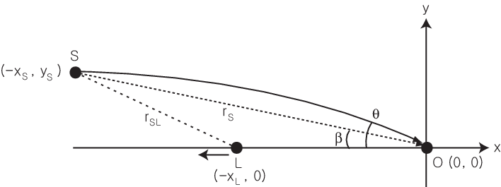
We consider the motion of a photon in the spacetime of (7) (FIG. 1). Corresponding Christoffel symbols can be calculated straightforwardly. Because of the symmetry of the system, we can confine the photon on the xx-yy plane and set z=0z=0. Also, the null condition

0=−(1−mR)+(1+mR)​{(x′−H​x)2+(y′−H​y)2},0=-\Big(1-\frac{m}{R}\Big)+\Big(1+\frac{m}{R}\Big)\{(x^{\prime}-Hx)^{2}+(y^{\prime}-Hy)^{2}\}\,, (8)

with a prime denoting a tt-derivative and R=(x+q​eH​t)2+y2R=\sqrt{(x+qe^{Ht})^{2}+y^{2}}, can be used to simplify geodesic equations. To reduce the number of equations to solve, we parametrize the geodesics by tt. Since tt is not an affine parameter, our geodesic equations have the following form:

xμ′′+Γμν​ρxν′xρ′=kxμ′.x^{\mu}{}^{\prime\prime}+\Gamma^{\mu}_{\nu\rho}x^{\nu}{}^{\prime}x^{\rho}{}^{\prime}=kx^{\mu}{}^{\prime}\,. (9)

With the help of (8), the tt-geodesic equation determines kk to be

k=H+mR3​{−H⁡(x2+y2)+x​x′+y​y′+eH​t​q​(x′−H​x)},k=H+\frac{m}{R^{3}}\{-H(x^{2}+y^{2})+xx^{\prime}+yy^{\prime}+e^{Ht}q(x^{\prime}-Hx)\}\,, (10)

and then xx- and yy-equations become

0\displaystyle 0 =\displaystyle= x′′−H​x′+mR3​{H​x′​(x2+y2)−(x​x′+y​y′)​x′+(x​y′−x′​y)​y′+eH​t​q​(H​x−x′)​(H​eH​t​q+2​x′)+eH​t​q},\displaystyle x^{\prime\prime}-Hx^{\prime}+\frac{m}{R^{3}}\Big\{Hx^{\prime}(x^{2}+y^{2})-(xx^{\prime}+yy^{\prime})x^{\prime}+(xy^{\prime}-x^{\prime}y)y^{\prime}+e^{Ht}q(Hx-x^{\prime})(He^{Ht}q+2x^{\prime})+e^{Ht}q\Big\}\,,
0\displaystyle 0 =\displaystyle= y′′−H​y′+mR3​{H​y′​(x2+y2)−(x​x′+y​y′)​y′−(x​y′−x′​y)​x′+eH​t​q​(H​y−y′)​(H​eH​t​q+2​x′)}.\displaystyle y^{\prime\prime}-Hy^{\prime}+\frac{m}{R^{3}}\Big\{Hy^{\prime}(x^{2}+y^{2})-(xx^{\prime}+yy^{\prime})y^{\prime}-(xy^{\prime}-x^{\prime}y)x^{\prime}+e^{Ht}q(Hy-y^{\prime})(He^{Ht}q+2x^{\prime})\Big\}\,. (11)

Next, we split the photon trajectory into the zeroth order piece(without L) and the first order one(with L, of 𝒪⁡(m){\cal O}(m)):

x=x0+mr​x1,y=y0+mr​y1,x=x_{0}+\frac{m}{r}x_{1}\,,\quad y=y_{0}+\frac{m}{r}y_{1}\,, (12)

where rr is the typical length scale of the lens system and r≫mr\gg m. The zeroth order solution is trivial:

x0=a1+a2​eH​t,y0=b1+b2​eH​t.x_{0}=a_{1}+a_{2}e^{Ht}\,,\quad y_{0}=b_{1}+b_{2}e^{Ht}\,. (13)

In the absence of the lens, the boundary conditions are such that at t=tSt=t_{\rm S} the photon was at the location of S, (−xS,yS)(-x_{\rm S},y_{\rm S}), and at t=tOt=t_{\rm O} it arrives at O at the origin, (0,0)(0,0). Then, a1a_{1}, a2a_{2}, b1b_{1}, b2b_{2} are fixed to be

a1=−eH​tO​xSeH​tO−eH​tS,a2=xSeH​tO−eH​tS,b1=eH​tO​ySeH​tO−eH​tS,b2=−ySeH​tO−eH​tS.\displaystyle a_{1}=-\frac{e^{Ht_{\rm O}}x_{\rm S}}{e^{Ht_{\rm O}}-e^{Ht_{\rm S}}}\,,\quad a_{2}=\frac{x_{\rm S}}{e^{Ht_{\rm O}}-e^{Ht_{\rm S}}}\,,\quad b_{1}=\frac{e^{Ht_{\rm O}}y_{\rm S}}{e^{Ht_{\rm O}}-e^{Ht_{\rm S}}}\,,\quad b_{2}=-\frac{y_{\rm S}}{e^{Ht_{\rm O}}-e^{Ht_{\rm S}}}\,. (14)

Plugging (12) and (13) into (11), we get the first order geodesic equations:

0\displaystyle 0 =\displaystyle= x1′′−H​x1′+(a12+b12)​(a2+q)+a1​eH​t​{(a2+q)2+b22}{(b1+b2​eH​t)2+(a1+eH​t​(a2+q))2}3/2​eH​t​H2​r,\displaystyle x_{1}^{\prime\prime}-Hx_{1}^{\prime}+\frac{(a_{1}^{2}+b_{1}^{2})(a_{2}+q)+a_{1}e^{Ht}\{(a_{2}+q)^{2}+b_{2}^{2}\}}{\{(b_{1}+b_{2}e^{Ht})^{2}+(a_{1}+e^{Ht}(a_{2}+q))^{2}\}^{3/2}}e^{Ht}H^{2}r\,,
0\displaystyle 0 =\displaystyle= y1′′−H​y1′+(a12+b12)​b2+b1​eH​t​{(a2+q)2+b22}{(b1+b2​eH​t)2+(a1+eH​t​(a2+q))2}3/2​eH​t​H2​r,\displaystyle y_{1}^{\prime\prime}-Hy_{1}^{\prime}+\frac{(a_{1}^{2}+b_{1}^{2})b_{2}+b_{1}e^{Ht}\{(a_{2}+q)^{2}+b_{2}^{2}\}}{\{(b_{1}+b_{2}e^{Ht})^{2}+(a_{1}+e^{Ht}(a_{2}+q))^{2}\}^{3/2}}e^{Ht}H^{2}r\,, (15)

whose solutions are

x1\displaystyle x_{1} =\displaystyle= c2+c1​eH​t+r​b2q​b1​(a1+eH​t​(a2+q))2+(b1+eH​t​b2)2\displaystyle c_{2}+c_{1}e^{Ht}+\frac{rb_{2}}{qb_{1}}\sqrt{(a_{1}+e^{Ht}(a_{2}+q))^{2}+(b_{1}+e^{Ht}b_{2})^{2}}
+r​eH​t​(a2+q)a12+b12​log⁡(e−H​t​H2​(a1​(a1+eH​t​(a2+q))+b1​(b1+eH​t​b2)CLOSECLOSE\displaystyle+\frac{re^{Ht}(a_{2}+q)}{\sqrt{a_{1}^{2}+b_{1}^{2}}}\log\Big(e^{-Ht}H^{2}\Big(a_{1}(a_{1}+e^{Ht}(a_{2}+q))+b_{1}(b_{1}+e^{Ht}b_{2})
OPENOPEN+a12+b12​(a1+eH​t​(a2+q))2+(b1+eH​t​b2)2)),\displaystyle\qquad\qquad\qquad+\sqrt{a_{1}^{2}+b_{1}^{2}}\sqrt{(a_{1}+e^{Ht}(a_{2}+q))^{2}+(b_{1}+e^{Ht}b_{2})^{2}}\;\Big)\Big)\,,
y1\displaystyle y_{1} =\displaystyle= d2+d1​eH​t−r⁡(a2+q)q​b1​(a1+eH​t​(a2+q))2+(b1+eH​t​b2)2\displaystyle d_{2}+d_{1}e^{Ht}-\frac{r(a_{2}+q)}{qb_{1}}\sqrt{(a_{1}+e^{Ht}(a_{2}+q))^{2}+(b_{1}+e^{Ht}b_{2})^{2}} (16)
+r​eH​t​b2a12+b12​log⁡(e−H​t​H2​(a1​(a1+eH​t​(a2+q))+b1​(b1+eH​t​b2)CLOSECLOSE\displaystyle+\frac{re^{Ht}b_{2}}{\sqrt{a_{1}^{2}+b_{1}^{2}}}\log\Big(e^{-Ht}H^{2}\Big(a_{1}(a_{1}+e^{Ht}(a_{2}+q))+b_{1}(b_{1}+e^{Ht}b_{2})
OPENOPEN+a12+b12​(a1+eH​t​(a2+q))2+(b1+eH​t​b2)2)).\displaystyle\qquad\qquad\qquad+\sqrt{a_{1}^{2}+b_{1}^{2}}\sqrt{(a_{1}+e^{Ht}(a_{2}+q))^{2}+(b_{1}+e^{Ht}b_{2})^{2}}\;\Big)\Big)\,.

When L is present, in order for a photon emitted at the source location to hit O at the origin, it should follow a bent trajectory, and the travel time is longer than tO−tSt_{\rm O}-t_{\rm S} by an amount of 𝒪⁡(m){\mathcal{O}}(m). Let us say it reaches the origin at t=tO+mr​t1t=t_{\rm O}+\frac{m}{r}t_{1}. Then, we need to fix six unknowns, c1c_{1}, c2c_{2}, d1d_{1}, d2d_{2}, qq and t1t_{1}, to completely determine the photon trajectory.

To be a trajectory of a photon (12) must satisfy the null condition: Plugging the solutions (13) and (16) into (8) gives

0=H2​(a12+b12)−1+mr​{A1​(t)​(a1​b2−a2​b1)+A2​(t)​(H2​(a12+b12)−1)+A3​(t)​(a1​c2+b1​d2)},0=H^{2}(a_{1}^{2}+b_{1}^{2})-1+\frac{m}{r}\{A_{1}(t)(a_{1}b_{2}-a_{2}b_{1})+A_{2}(t)(H^{2}(a_{1}^{2}+b_{1}^{2})-1)+A_{3}(t)(a_{1}c_{2}+b_{1}d_{2})\}\,, (17)

where AiA_{i}’s are some complicated functions of tt. Then, at 𝒪⁡(m0){\mathcal{O}}(m^{0}), we get

H2​(a12+b12)=1⇒e−H⁡(tO−tS)=1−H​rS,H^{2}(a_{1}^{2}+b_{1}^{2})=1\quad\Rightarrow\quad e^{-H(t_{\rm O}-t_{\rm S})}=1-Hr_{\rm S}\,, (18)

which relates the source-observer time difference, tO−tSt_{\rm O}-t_{\rm S}, to the source-observer distance, rS=xS2+yS2r_{\rm S}=\sqrt{x_{\rm S}^{2}+y_{\rm S}^{2}}, in the absence of the lens. Next at 𝒪⁡(m){\mathcal{O}}(m) we have

a1​c2+b1​d2=0,a_{1}c_{2}+b_{1}d_{2}=0\,, (19)

and this is our first constraint on the unknowns. Note that (18) can be generalized by considering (8) at 𝒪⁡(m0){\mathcal{O}}(m^{0}):

1+H​x=d​xd​t⇒H⁡(tO−t∙)=log⁡(1+H​xO)−log⁡(1+H​x∙)=−log⁡(1+H​x∙),1+Hx=\frac{{\rm d}x}{{\rm d}t}\quad\Rightarrow\quad H(t_{\rm O}-t_{\bullet})=\log(1+Hx_{\rm O})-\log(1+Hx_{\bullet})=-\log(1+Hx_{\bullet})\,, (20)

where x∙x_{\bullet} is the location of the photon at t=t∙t=t_{\bullet}. The boundary conditions in the presence of the lens give 4 constraints:

x⁡(tS)=−xS=−xS+mr​x1​(tS),\displaystyle x(t_{\rm S})=-x_{\rm S}=-x_{\rm S}+\frac{m}{r}x_{1}(t_{\rm S})\,,\quad x⁡(tO+mr​t1)=0=x0′​(tO)​mr​t1+mr​x1​(tO),\displaystyle x(t_{\rm O}+\frac{m}{r}t_{1})=0=x_{0}^{\prime}(t_{\rm O})\frac{m}{r}t_{1}+\frac{m}{r}x_{1}(t_{\rm O})\,, (21)
y⁡(tS)=yS=yS+mr​y1​(tS),\displaystyle y(t_{\rm S})=y_{\rm S}=y_{\rm S}+\frac{m}{r}y_{1}(t_{\rm S})\,,\quad y⁡(tO+mr​t1)=0=y0′​(tO)​mr​t1+mr​y1​(tO).\displaystyle y(t_{\rm O}+\frac{m}{r}t_{1})=0=y_{0}^{\prime}(t_{\rm O})\frac{m}{r}t_{1}+\frac{m}{r}y_{1}(t_{\rm O})\,.

The last piece of information necessary for connecting our algebra to the observation is the location of L: it was located at −rL-r_{\rm L} at time t=tLt=t_{\rm L}. In order for us to detect it at t=tOt=t_{\rm O}, rLr_{\rm L} and tLt_{\rm L} must satisfy (20), i.e.,

e−H⁡(tO−tL)=1−H​rL.e^{-H(t_{\rm O}-t_{\rm L})}=1-Hr_{\rm L}\,. (22)

Then qq can be determined by

−q​eH​tL=−rL⇒q=e−H​tO​rL1−H​rL≡e−H​tO​xL.-qe^{Ht_{\rm L}}=-r_{\rm L}\quad\Rightarrow\quad q=e^{-Ht_{\rm O}}\frac{r_{\rm L}}{1-Hr_{\rm L}}\equiv e^{-Ht_{\rm O}}x_{\rm L}\,. (23)

With (14), (18) and (23), solving (19) and (21) gives the rest of the unknowns:

c1\displaystyle c_{1} =\displaystyle= r​e−H​tSH​rS3​xL[rS{−H2rSxL2xS+(H(rS2−xLxS)−rS)(−xL+(xS−(1−H​rS)​xL)2+yS2)}\displaystyle\frac{re^{-Ht_{\rm S}}}{Hr_{\rm S}^{3}x_{\rm L}}\Big[\,r_{\rm S}\Big\{-H^{2}r_{\rm S}x_{\rm L}^{2}x_{\rm S}+\Big(H(r_{\rm S}^{2}-x_{\rm L}x_{\rm S})-r_{\rm S}\Big)\Big(-x_{\rm L}+\sqrt{(x_{\rm S}-(1-Hr_{\rm S})x_{\rm L})^{2}+y_{\rm S}^{2}}\;\Big)\Big\}
−H(1−HrS)xL{rS2(HrSxL+xS)loge−H​tS​H​(1−H​rS)​(rS−xS)​xLrS\displaystyle\quad-H(1-Hr_{\rm S})x_{\rm L}\Big\{r_{\rm S}^{2}(Hr_{\rm S}x_{\rm L}+x_{\rm S})\log\frac{e^{-Ht_{\rm S}}H(1-Hr_{\rm S})(r_{\rm S}-x_{\rm S})x_{\rm L}}{r_{\rm S}}
+(rS2(HrSxL+xS)−xLyS2)logrS2−xL​xS​(1−H​rS)+rS​(xS−(1−H​rS)​xL)2+yS2(1−H​rS)​(rS−xS)​xL}],\displaystyle\qquad+\Big(r_{\rm S}^{2}(Hr_{\rm S}x_{\rm L}+x_{\rm S})-x_{\rm L}y_{\rm S}^{2}\Big)\log\frac{r_{\rm S}^{2}-x_{\rm L}x_{\rm S}(1-Hr_{\rm S})+r_{\rm S}\sqrt{(x_{\rm S}-(1-Hr_{\rm S})x_{\rm L})^{2}+y_{\rm S}^{2}}}{(1-Hr_{\rm S})(r_{\rm S}-x_{\rm S})x_{\rm L}}\;\Big\}\,\Big]\,,
c2\displaystyle c_{2} =\displaystyle= rH​rS3​xL[rS(rS+HxSxL){−xL(1−HrS)+(xS−(1−H​rS)​xL)2+yS2}\displaystyle\frac{r}{Hr_{\rm S}^{3}x_{\rm L}}\Big[\,r_{\rm S}(r_{\rm S}+Hx_{\rm S}x_{\rm L})\Big\{-x_{\rm L}(1-Hr_{\rm S})+\sqrt{(x_{\rm S}-(1-Hr_{\rm S})x_{\rm L})^{2}+y_{\rm S}^{2}}\;\Big\} (24)
−H(1−HrS)xL2yS2logrS2−xL​xS​(1−H​rS)+rS​(xS−(1−H​rS)​xL)2+yS2(1−H​rS)​(rS−xS)​xL],\displaystyle\quad-H(1-Hr_{\rm S})x_{\rm L}^{2}y_{\rm S}^{2}\log\frac{r_{\rm S}^{2}-x_{\rm L}x_{\rm S}(1-Hr_{\rm S})+r_{\rm S}\sqrt{(x_{\rm S}-(1-Hr_{\rm S})x_{\rm L})^{2}+y_{\rm S}^{2}}}{(1-Hr_{\rm S})(r_{\rm S}-x_{\rm S})x_{\rm L}}\;\Big]\,,
d1\displaystyle d_{1} =\displaystyle= r​e−H​tSH​rS3​xL​yS[rS{H2rSxL2yS2+(H(rS2xS−xLxS2)−rSxS+H2rS3xL)(−xL+(xS−(1−H​rS)​xL)2+yS2)}\displaystyle\frac{re^{-Ht_{\rm S}}}{Hr_{\rm S}^{3}x_{\rm L}y_{\rm S}}\Big[\,r_{\rm S}\Big\{H^{2}r_{\rm S}x_{\rm L}^{2}y_{\rm S}^{2}+\Big(H(r_{\rm S}^{2}x_{\rm S}-x_{\rm L}x_{\rm S}^{2})-r_{\rm S}x_{\rm S}+H^{2}r_{\rm S}^{3}x_{\rm L}\Big)\Big(-x_{\rm L}+\sqrt{(x_{\rm S}-(1-Hr_{\rm S})x_{\rm L})^{2}+y_{\rm S}^{2}}\;\Big)\Big\}
+H(1−HrS)xLyS2{rS2loge−H​tS​H​(1−H​rS)​(rS−xS)​xLrS\displaystyle\quad+H(1-Hr_{\rm S})x_{\rm L}y_{\rm S}^{2}\Big\{r_{\rm S}^{2}\log\frac{e^{-Ht_{\rm S}}H(1-Hr_{\rm S})(r_{\rm S}-x_{\rm S})x_{\rm L}}{r_{\rm S}}
+(rS2+xLxS)logrS2−xL​xS​(1−H​rS)+rS​(xS−(1−H​rS)​xL)2+yS2(1−H​rS)​(rS−xS)​xL}],\displaystyle\qquad+(r_{\rm S}^{2}+x_{\rm L}x_{\rm S})\log\frac{r_{\rm S}^{2}-x_{\rm L}x_{\rm S}(1-Hr_{\rm S})+r_{\rm S}\sqrt{(x_{\rm S}-(1-Hr_{\rm S})x_{\rm L})^{2}+y_{\rm S}^{2}}}{(1-Hr_{\rm S})(r_{\rm S}-x_{\rm S})x_{\rm L}}\;\Big\}\Big]\,,
d2\displaystyle d_{2} =\displaystyle= −a1b1​c2,\displaystyle-\frac{a_{1}}{b_{1}}c_{2}\,,

and

t1\displaystyle t_{1} =\displaystyle= r1−H​rS{H(−(1−HrS)xL+(xS−(1−H​rS)​xL)2+yS2)\displaystyle\frac{r}{1-Hr_{\rm S}}\Big\{H\Big(-(1-Hr_{\rm S})x_{\rm L}+\sqrt{(x_{\rm S}-(1-Hr_{\rm S})x_{\rm L})^{2}+y_{\rm S}^{2}}\;\Big) (25)
+(1−HrS)(1+HxLxSrS)logrS2−xL​xS​(1−H​rS)+rS​(xS−(1−H​rS)​xL)2+yS2(1−H​rS)​(rS−xS)​xL}.\displaystyle+(1-Hr_{\rm S})\Big(1+Hx_{\rm L}\frac{x_{\rm S}}{r_{\rm S}}\Big)\log\frac{r_{\rm S}^{2}-x_{\rm L}x_{\rm S}(1-Hr_{\rm S})+r_{\rm S}\sqrt{(x_{\rm S}-(1-Hr_{\rm S})x_{\rm L})^{2}+y_{\rm S}^{2}}}{(1-Hr_{\rm S})(r_{\rm S}-x_{\rm S})x_{\rm L}}\;\Big\}\,.

With (24) and (25), we can see that x1x_{1}, y1y_{1} and t1t_{1} have an overall factor of rr, so that the arbitrary parameter rr does not appear in the full solution. t1t_{1} has a special implication: mr​t1\frac{m}{r}t_{1} is related to the time delay due to the lens.

Now that the photon trajectory is determined, we can calculate the angular location of the image of S observed by us:

θ\displaystyle\theta =\displaystyle= −tan−1⁡y′x′|tO+mr​t1\displaystyle-\tan^{-1}\frac{y^{\prime}}{x^{\prime}}\Big|_{\,t_{\rm O}+\frac{m}{r}t_{1}} (26)
=\displaystyle= β+mxL​yS{xS+HrSxL+(1+HxLxSrS)(−(1−HrS)xL+(xS−(1−H​rS)​xL)2+yS2)\displaystyle\beta+\frac{m}{x_{\rm L}y_{\rm S}}\Big\{x_{\rm S}+Hr_{\rm S}x_{\rm L}+\Big(1+Hx_{\rm L}\frac{x_{\rm S}}{r_{\rm S}}\Big)\Big(-(1-Hr_{\rm S})x_{\rm L}+\sqrt{(x_{\rm S}-(1-Hr_{\rm S})x_{\rm L})^{2}+y_{\rm S}^{2}}\;\Big)
−yS2rS2HxL2(1−HrS)logrS2−xL​xS​(1−H​rS)+rS​(xS−(1−H​rS)​xL)2+yS2(1−H​rS)​(rS−xS)​xL}+𝒪(m2),\displaystyle\qquad\qquad-\frac{y_{\rm S}^{2}}{r_{\rm S}^{2}}Hx_{\rm L}^{2}(1-Hr_{\rm S})\log\frac{r_{\rm S}^{2}-x_{\rm L}x_{\rm S}(1-Hr_{\rm S})+r_{\rm S}\sqrt{(x_{\rm S}-(1-Hr_{\rm S})x_{\rm L})^{2}+y_{\rm S}^{2}}}{(1-Hr_{\rm S})(r_{\rm S}-x_{\rm S})x_{\rm L}}\,\Big\}+{\mathcal{O}}(m^{2})\,,

where β=tan−1⁡ySxS\beta=\tan^{-1}\frac{y_{\rm S}}{x_{\rm S}} is the undeflected image location, and xL=rL/(1−H​rL)x_{\rm L}=r_{\rm L}/(1-Hr_{\rm L}). This is the exact result up to 𝒪⁡(m){\mathcal{O}}(m).

Refer to caption
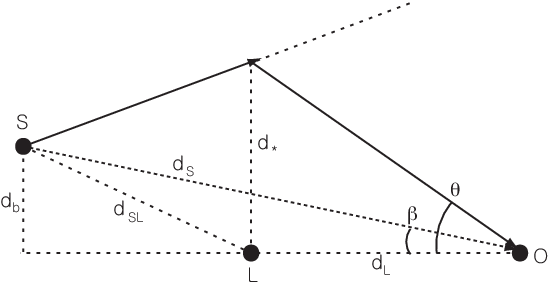
Figure 2: Lensing schematics in conventional analysis

On the other hand the conventional lensing analysis(FIG. 2), e.g., § IV of [7], gives

θc≈βc+2​m​dSLβc​dL​dS+𝒪⁡(m2),\theta_{c}\approx\beta_{c}+\frac{2md_{\rm SL}}{\beta_{c}d_{\rm L}d_{\rm S}}+{\cal O}(m^{2})\,, (27)

where d∙d_{\bullet}’s are angular diameter distances defined by d∙=a⁡(t∙)​ρ∙d_{\bullet}=a(t_{\bullet})\rho_{\bullet} with ρ∙\rho_{\bullet} being the corresponding comoving distance. Obviously

βc≈dbdS,θc≈d∗dL.\beta_{c}\approx\frac{d_{b}}{d_{\rm S}}\,,\quad\theta_{c}\approx\frac{d_{*}}{d_{\rm L}}\,. (28)

To compare (27) to our result (26), we first note that our xSx_{\rm S}, ySy_{\rm S} and rSr_{\rm S} are distances at t=tSt=t_{\rm S} and rLr_{\rm L} at t=tLt=t_{\rm L}. Then from (6), we immediately see that these are the same as the angular diameter distances, i.e., rS=dSr_{\rm S}=d_{\rm S}, rL=dLr_{\rm L}=d_{\rm L}, and therefore βc=β\beta_{c}=\beta, θc=θ\theta_{c}=\theta. Now for small HH, (26) becomes

θ=β+2​mβ​dS​dL​{xS−dL+H​dL​(xS−dL)+H2​dL2​(xS−dL)+𝒪⁡(H3)+𝒪⁡(β2)}+𝒪⁡(m2).\theta=\beta+\frac{2m}{\beta d_{\rm S}d_{\rm L}}\Big\{x_{\rm S}-d_{\rm L}+Hd_{\rm L}(x_{\rm S}-d_{\rm L})+H^{2}d_{\rm L}^{2}(x_{\rm S}-d_{\rm L})+{\mathcal{O}}(H^{3})+{\mathcal{O}}(\beta^{2})\Big\}+{\mathcal{O}}(m^{2})\,. (29)

Using

dSL\displaystyle d_{\rm SL} =\displaystyle= a⁡(tS)​(xSa⁡(tS)−dLa⁡(tL))2+(ySa⁡(tS))2=(xS−1−H​ds1−H​dL​dL)2+yS2\displaystyle a(t_{\rm S})\sqrt{\Big(\frac{x_{\rm S}}{a(t_{\rm S})}-\frac{d_{\rm L}}{a(t_{\rm L})}\Big)^{2}+\Big(\frac{y_{\rm S}}{a(t_{\rm S})}\Big)^{2}}=\sqrt{\Big(x_{\rm S}-\frac{1-Hd_{\rm s}}{1-Hd_{\rm L}}d_{\rm L}\Big)^{2}+y_{\rm S}^{2}} (30)
=\displaystyle= xS−dL+H​dL​(xS−dL)+H2​dL2​(xS−dL)+𝒪⁡(H3)+𝒪⁡(β2),\displaystyle x_{\rm S}-d_{\rm L}+Hd_{\rm L}(x_{\rm S}-d_{\rm L})+H^{2}d_{\rm L}^{2}(x_{\rm S}-d_{\rm L})+{\mathcal{O}}(H^{3})+{\mathcal{O}}(\beta^{2})\,,

we can rewrite (29) as

θ=β+2​m​dSLβ​dS​dL​(1+𝒪⁡(H3)+𝒪⁡(β2))+𝒪⁡(m2),\theta=\beta+\frac{2md_{\rm SL}}{\beta d_{\rm S}d_{\rm L}}\Big(1+{\cal O}(H^{3})+{\cal O}(\beta^{2})\Big)+{\cal O}(m^{2})\,, (31)

where

𝒪⁡(β2)=−β2​xS2−4​xS​dL+2​dL24​(xS−dL)+⋯.{\cal O}(\beta^{2})=-\beta^{2}\frac{x_{\rm S}^{2}-4x_{\rm S}d_{\rm L}+2d_{\rm L}^{2}}{4(x_{\rm S}-d_{\rm L})}+\cdots\,. (32)

Therefore, our result is in contradiction to the recent claims by [3] which assert that there should be a 𝒪⁡(Λ)∼𝒪⁡(H2){\mathcal{O}}(\Lambda)\sim{\mathcal{O}}(H^{2}) correction to the conventional lensing analysis.

III Discussion

Through rigorous, close-to-the-reality but laborious derivations, we confirm that the conventional gravitational lensing analysis, although it may look loosely constructed, is actually accurate, at least for thin, weak lenses in a Λ\Lambda driven universe. [6], which incorporated the “reality” in their analysis by employing FRW coordinates, has the same conclusion as ours.

The differences between our work and [3]-[4](and [5]) can originate from the following: In [3],

  1. 1.

    the setup is not describing the actual observation: In the SdS universe, L and O must be moving relative to each other due to Hubble expansion, whereas they got an angle measured by an observer with fixed coordinates,

  2. 2.

    their result is not written in terms of angular diameter distances, which are necessary to compare with the conventional results.

In their follow-up paper [4], some effort was made to take these into consideration. But

  • •

    their method to resolve problem 2, i.e., employing the Einstein-Strauss scheme or the lens equation, does not seem to be used properly: They are necessary in the Schwarzschild lensing because the Hubble expansion, which is not considered in the calculation of the bending angle, has to be implemented. On the other hand, the SdS spacetime is a complete playground for gravitational lensing because the metric is equivalent to the McVittie solution which already knows about both the lens and FRW. Then appropriate specifications of O, L and S should be enough for the full description of phenomena. Obviously, using Einstein-Strauss scheme or the lens equation together with SdS background is redundant.

  • •

    the problem 1 was not addressed: Their angle ψ\psi(in the first paper) or α\alpha(in the second paper) is measured by a static observer(O). The instantaneous speed vv of a geodesically moving observer(O′\prime) can be calculated to be

    v=mrL+H2​rL2,v=\sqrt{\frac{m}{r_{L}}+H^{2}r_{L}^{2}}\,, (33)

    where rLr_{L} is the radial coordinate of O(O′\prime) at the moment of the observation. Then, by relativistic aberration, the angle observed by O′\prime is

    ψ′=1+v1−v​ψ,\psi^{\prime}=\sqrt{\frac{1+v}{1-v}}\psi\,, (34)

    assuming ψ⁡(ψ′)\psi(\psi^{\prime}) is small. To get the final result, we should convert quantities appearing in (34) into angular diameter distances. This last step could be tricky, which makes the intuitive setup presented in the previous section favorable.

The same rigorous procedure can be applied to generic FRW systems. For example, in the case of matter domination with a⁡(t)∼t2/3a(t)\sim t^{2/3}, once finishing tremendously more complicated intermediate steps, we can write the final result as

θ=β+2​mβ​dS​dL​{xS−dL+23​tO​dL​(xS−dL)+(23​tO)2​dL​(xS−dL)​3​xS+7​dL4+𝒪​(23​tO)3+𝒪⁡(β2)}+𝒪⁡(m2).\theta=\beta+\frac{2m}{\beta d_{\rm S}d_{\rm L}}\Big\{x_{\rm S}-d_{\rm L}+\frac{2}{3t_{\rm O}}d_{\rm L}(x_{\rm S}-d_{\rm L})+\Big(\frac{2}{3t_{\rm O}}\Big)^{2}d_{\rm L}(x_{\rm S}-d_{\rm L})\frac{3x_{\rm S}+7d_{\rm L}}{4}+{\mathcal{O}}\Big(\frac{2}{3t_{\rm O}}\Big)^{3}+{\mathcal{O}}(\beta^{2})\Big\}+{\mathcal{O}}(m^{2})\,. (35)

After relating dSLd_{\rm SL} to other variables in a similar way as (30), we get

θ=β+2​m​dSLβ​dS​dL​(1+𝒪⁡(HO3)+𝒪⁡(β2))+𝒪⁡(m2),\theta=\beta+\frac{2md_{\rm SL}}{\beta d_{\rm S}d_{\rm L}}\Big(1+{\mathcal{O}}(H_{\rm O}^{3})+{\mathcal{O}}(\beta^{2})\Big)+{\mathcal{O}}(m^{2})\,, (36)

with HO=2/(3​tO)H_{\rm O}=2/(3t_{\rm O}), which still ascertains the accuracy of the conventional analysis.

In addition to confirming the conventional results, our work can provide the exact formulae for errors coming from dropping higher order terms of 𝒪⁡(HO3){\mathcal{O}}(H_{\rm O}^{3}) and 𝒪⁡(β2){\mathcal{O}}(\beta^{2}), which might have importance in testing theories of long-range modification of gravity: Since our results are obtained under the assumption that the general relativity(GR) is valid up to any scale, if precise measurements of high redshift lensing systems differ from our prediction, it may indicate that GR needs some modifications at large distances. At present, these theoretical errors are well buried beneath the measurement ones, but as our observational tools develop they may become significant in the future.

Acknowledgement

We thank C. Fassnacht, A. Iglesias, C. Keeton and especially N. Kaloper for discussions.

References

  • [1] G. C. McVittie, Mon. Not. R. Astron. Soc. 93 (1933) 325.
  • [2] J. N. Islam, Phys.Lett. A 97, 239 (1983); W. H. C. Freire, V. B. Bezerra and J. A. S. Lima, Gen. Rel. Grav. 33, 1407 (2001), arXiv:gr-qc/0201036; K. Lake, Phys. Rev. D 65, 087301 (2002); A. W. Kerr, J. C. Hauck and B. Mashhoon, Class. Quant. Grav. 20, 2727 (2003), arXiv:gr-qc/0301057; F. Finelli, M. Galaverni and A. Gruppuso, Phys. Rev. D 75, 043003 (2007), arXiv:astro-ph/0601044; V. Kagramanova, J. Kunz and C. Lammerzahl, Phys. Lett. B 634, 465 (2006), arXiv:gr-qc/0602002.
  • [3] W. Rindler and M. Ishak, Phys. Rev. D 76, 043006 (2007), arXiv:0709.2948 [astro-ph];
  • [4] M. Ishak, W. Rindler, J. Dossett, J. Moldenhauer and C. Allison, arXiv:0710.4726 [astro-ph].
  • [5] K. Lake, arXiv:0711.0673 [gr-qc]; M. Sereno, Phys. Rev. D 77, 043004 (2008),
    arXiv:0711.1802 [astro-ph]; T. Schucker, arXiv:0712.1559 [astro-ph]; M. Ishak, arXiv:0801.3514 [astro-ph]; T. Schucker and N. Zaimen, arXiv:0801.3776 [astro-ph].
  • [6] I. B. Khriplovich and A. A. Pomeransky, arXiv:0801.1764 [gr-qc].
  • [7] C. R. Keeton and A. O. Petters, Phys. Rev. D 72, 104006 (2005), arXiv:gr-qc/0511019.